The physics in Oppenheimer

A literature review, scene by scene

Published

October 24, 2026

Abstract

Christopher Nolan’s Oppenheimer (2023) moves through about thirty years of physics: molecular quantum mechanics in 1927, neutron stars and gravitational collapse in 1939, fission, the bomb, and the hydrogen bomb debate. This review collects what historians and physicists have written about the film, then takes each piece of physics in the order the film meets it. For each one it gives the paper or report where the work first appeared, the key equations, and a short calculation that checks the numbers.

Note

Written by Claude as a reading guide. Every journal article in the bibliography was checked against Crossref, and every textbook section number against the book. Scene descriptions come from memory of the film and from the reviews cited, so check any claim about what is on screen against the film itself. Calculations use textbook models and stated inputs; they reproduce orders of magnitude and some classic results, not design figures.

1 How to read the film’s physics

The film covers three periods, and each one leaves a different paper trail.

1926 to 1939: open literature. Everything Oppenheimer and his contemporaries did before the war appeared in ordinary journals: Zeitschrift für Physik, Annalen der Physik, Physical Review, Nature. These are the papers to read alongside the early scenes. The issue of Physical Review dated 1 September 1939, the day Germany invaded Poland, holds both Bohr and Wheeler’s theory of fission (Bohr and Wheeler 1939) and Oppenheimer and Snyder’s paper on collapse (Oppenheimer and Snyder 1939).

1940 to 1945: secrecy. Physicists in Britain and the United States began holding back fission results in 1940, before any government required it. The system leaked at first. McMillan and Abelson published the discovery of neptunium in June 1940 (McMillan and Abelson 1940), and Flerov and Petrzhak published spontaneous fission in Physical Review that summer (Flerov and Petrjak 1940). By 1941 the controls held: Seaborg, McMillan, Kennedy and Wahl’s letter on element 94 reached Physical Review on 28 January 1941 and waited until 1946 (Seaborg et al. 1946). Wartime work went into numbered Los Alamos reports instead: LA-1 (Serber’s lectures, published as Serber (1992)) and LA-602 on atmospheric ignition (Konopinski et al. 1946). Wellerstein (2021) tells the story of this system.

1945 onward: release in stages. The Smyth Report (Smyth 1945) was the first official account. The withheld papers followed in 1946 (Seaborg et al. 1946; Kennedy et al. 1946), and the Los Alamos reports came out over decades. Some details of weapon design remain classified. Academics also worked results out from the outside: G. I. Taylor estimated the Trinity yield in 1950 from published photographs (Taylor 1950a, 1950b), which Section 12 repeats.

So “the original paper” means a journal article for the scenes up to 1939, an internal report for the Los Alamos scenes, and often a post-war reconstruction for the bomb physics itself. Reed (2021) rebuilds that physics from open sources and is the best single companion to the middle of the film. Hoddeson et al. (1993) is the technical history of Los Alamos.

2 What reviewers said

No full-length scholarly study of the film’s physics has appeared. The closest pieces are reviews and letters.

Historians. Whitfield (2024) reviews the film for the Journal of American History. He reads it as narrowing a large scientific and political effort down to one man. Griffith (2023) goes scene by scene for the Bulletin of the Atomic Scientists and finds the technical content mostly faithful. He calls the marbles-in-bowls scene invented, though it conveys the scale of the isotope problem. He notes that Rutherford, not Blackett, introduced Oppenheimer to Bohr, and that the film gives the atmospheric-ignition question more weight than it had in 1945. Greenberg and Tuquero (2023) found that the two Einstein scenes about ignition did not happen; Oppenheimer took the question to Arthur Compton.

Physicists. A Physics Today exchange set the terms of the debate. Santiago and Rand (2024) argue that the film celebrates Trinity as a scientific feat and ignores fallout and the people living downwind. Reed (2024) answers that the film is a life of Oppenheimer, not a documentary, and that it may draw young viewers to the history. Reed is the author of Reed (2021). The writers at Physics World (Durrani et al. 2023) rated the film highly; Kate Gardner also raised the people living near the test site. Scientists at ANSTO wanted more physics on screen (ANSTO 2023). Kevin Pitts checked the delay between the Trinity flash and the sound and found it right (Virginia Tech News 2023). In an interview with Science, the historian David Cassidy called Oppenheimer “no Einstein” but rated the collapse work at Nobel level (Cho 2023). Los Alamos published its own summary of his science (Los Alamos National Laboratory 2023).

On the physics itself. Ortega-Rodríguez et al. (2017) is the best paper on why the collapse work of 1939 went unused for two decades. It sits between history and physics and does not depend on the film.

3 Göttingen, 1927: separating electrons from nuclei

The film shows Oppenheimer arriving in Göttingen to work with Max Born. Two papers came out of that year: his thesis on the continuous spectrum (Oppenheimer 1927) and the paper with Born that every chemistry course still uses (Born and Oppenheimer 1927).

A molecule has electrons at positions \(\mathbf r\) and nuclei at positions \(\mathbf R\), with Hamiltonian \[ H = T_N + T_e + V(\mathbf r, \mathbf R), \qquad T_N = -\sum_a \frac{\hbar^2}{2M_a}\nabla_a^2 . \] Nuclei are thousands of times heavier than electrons and move slowly, so Born and Oppenheimer first solve for the electrons with the nuclei held still: \[ \bigl[T_e + V(\mathbf r; \mathbf R)\bigr]\,\phi_k(\mathbf r; \mathbf R) = U_k(\mathbf R)\,\phi_k(\mathbf r; \mathbf R). \] The electronic energy \(U_k(\mathbf R)\) then acts as the potential for the nuclei: \[ \bigl[T_N + U_k(\mathbf R)\bigr]\,\chi(\mathbf R) = E\,\chi(\mathbf R), \qquad \Psi(\mathbf r, \mathbf R) \approx \phi_k(\mathbf r; \mathbf R)\,\chi(\mathbf R). \] Born and Oppenheimer expanded in the small parameter \(\kappa = (m_e/M)^{1/4}\) and found the familiar ordering of molecular energies: \[ E_{\text{electronic}} : E_{\text{vibration}} : E_{\text{rotation}} \approx 1 : \kappa^2 : \kappa^4 . \]

Code

kappa = (m_e / m_p) ** 0.25
print(f"H2: kappa = {kappa:.3f}, kappa^2 = {kappa**2:.4f}, "
      f"kappa^4 = {kappa**4:.5f}")

H2: kappa = 0.153, kappa^2 = 0.0233, kappa^4 = 0.00054

For hydrogen, with \(M = m_p\), that gives \(\kappa \approx\) 0.15: vibrational energies a few per cent of electronic ones, rotational energies a few parts in ten thousand. That matches spectra (electronic transitions in the ultraviolet, vibrations in the infrared, rotations in the microwave).

Textbooks: Landau and Lifshitz (1977, sec. 78), Tong (2017, sec. 2.3.6), and Shankar (1994, sec. 21.1, under “The Berry Phase”), which derives the separation from the path integral.

4 Heisenberg’s lecture: uncertainty

The film puts Oppenheimer, with Rabi, in the audience for a Heisenberg lecture. The paper of that year is Heisenberg (1927), which argued from thought experiments that position and momentum cannot both be exact, roughly \(\delta x\,\delta p \sim h\). The inequality in its modern form, \[ \sigma_x \sigma_p \ge \frac{\hbar}{2}, \] with \(\sigma\) the standard deviation, came from Kennard (1927) soon after.

Textbooks: Landau and Lifshitz (1977, sec. 16), Tong (n.d.-b, sec. 3.4.1) and Shankar (1994, ch. 9).

5 Berkeley in the 1930s

The film compresses Oppenheimer’s Berkeley years into a few scenes of teaching and of Lawrence’s Radiation Laboratory. The physics behind them is mostly not on screen, but it explains his reputation.

5.1 Tunnelling

Oppenheimer (1928) includes one of the first uses of quantum tunnelling: an electric field \(F\) can pull the electron out of a hydrogen atom even though classically it is bound. In the WKB approximation the probability of crossing a barrier is \[ T \approx \exp\!\left(-\frac{2}{\hbar}\int \sqrt{2m\,[V(x) - E]}\,\mathrm dx\right), \] and for an electron bound by energy \(W\) in a uniform field, the barrier \(V - E = W - eFx\) is a triangle, giving \[ T \approx \exp\!\left(-\frac{4\sqrt{2m}\,W^{3/2}}{3\hbar e F}\right). \] The same exponent governs field emission from metals (Fowler and Nordheim, also 1928).

Textbooks: barrier penetration is in Landau and Lifshitz (1977, sec. 50), and the ionisation of hydrogen by an electric field, the problem Oppenheimer tackled, is worked in Landau and Lifshitz (1977, sec. 77, Problem 1). Tong (2017, secs. 2.2.5, 4.1) and Shankar (1994, sec. 16.2) cover the same ground.

5.2 The anti-electron

Dirac’s equation allows negative energies, \(E = \pm\sqrt{p^2c^2 + m^2c^4}\). Dirac first suggested that the “holes” in the filled sea of negative-energy states were protons. Oppenheimer (1930) pointed out that the electron in a hydrogen atom would then fall into its proton’s hole, so hydrogen would annihilate within a tiny fraction of a second. Weyl showed in the same period that the theory’s symmetry forces the hole to have the electron’s mass. Dirac (1931) accepted both points and predicted the anti-electron, which Anderson (1933) found in cosmic rays.

Textbooks: Tong (2006, sec. 5.3), Tong (n.d.-a, sec. 2.1.3) and Shankar (1994, sec. 20.3). Tong (n.d.-a) explains why the Dirac sea, though it led to the right prediction, is the wrong picture. Berestetskii et al. (1982) treat antiparticles without the sea [§11] and give Dirac’s equation [§§20–21]. The annihilation behind Oppenheimer’s argument is worked out there as two-photon annihilation of an electron pair (Berestetskii et al. 1982, sec. 88).

5.3 Deuterons and the Coulomb barrier

A charged particle hitting a nucleus must climb the Coulomb barrier, \[ V_C = \frac{Z_1 Z_2 e^2}{4\pi\varepsilon_0\,R}, \qquad R \approx r_0\bigl(A_1^{1/3} + A_2^{1/3}\bigr),\quad r_0 \approx 1.2~\text{fm}. \] Oppenheimer and Phillips (1935) explained why deuterons react with heavy nuclei at energies below this barrier. The deuteron is large and loosely bound (2.2 MeV). The nucleus repels its proton, which leaves the neutron in front to be captured while the proton flies off. This (d, p) reaction is the Oppenheimer–Phillips process.

Textbooks: Landau and Lifshitz (1977, sec. 50, Problem 2) derive the tunnelling factor through a Coulomb barrier, first found by Gamow. Krane (1988, sec. 8.4) uses it for alpha decay, and covers the deuteron in §4.1 and stripping reactions in §11.11.

5.4 Lawrence’s cyclotron

A charge \(q\) in a field \(B\) circles at the cyclotron frequency, which does not depend on its speed: \[ \omega_c = \frac{qB}{m}, \qquad K_{\max} = \frac{q^2 B^2 R^2}{2m}, \] so a fixed-frequency oscillator can kick it twice per turn as it spirals out to the magnet’s radius \(R\) (Lawrence and Livingston 1932). The same magnets later became the calutrons of Section 9.

Textbooks: Landau and Lifshitz (1975, sec. 21), Tong (2013, sec. 2.4.2) and Krane (1988, sec. 15.2).

6 Stars, 1938–1939: neutron cores and collapse

The film gives one scene to this work: Oppenheimer and Hartland Snyder talking through what happens when a star exhausts its fuel. It is the work modern physicists rate highest (Cho 2023; Ortega-Rodríguez et al. 2017).

6.1 The sequence of papers

Landau (1938) proposed that stars might have neutron cores. Oppenheimer and Serber (1938) showed that such cores are unstable unless they are large. Tolman (1939) and Oppenheimer and Volkoff (1939), back to back in Physical Review, set up the general-relativistic equations of stellar structure and found a maximum mass for a star held up by neutron degeneracy pressure. Oppenheimer and Snyder (1939) then asked what happens above it.

6.2 The Tolman–Oppenheimer–Volkoff equation

For a static, spherically symmetric star with pressure \(P(r)\), mass-energy density \(\varepsilon(r)\) and enclosed mass \(m(r)\), general relativity replaces Newtonian hydrostatic equilibrium with \[ \frac{\mathrm dP}{\mathrm dr} = -\frac{G\,\bigl(\varepsilon/c^2 + P/c^2\bigr)\bigl(m + 4\pi r^3 P/c^2\bigr)} {r^2\bigl(1 - 2Gm/rc^2\bigr)}, \qquad \frac{\mathrm dm}{\mathrm dr} = \frac{4\pi r^2 \varepsilon}{c^2}. \] Each of the three corrections to Newton makes gravity stronger: pressure gravitates, it adds to the enclosed mass, and the metric factor diverges as \(r \to 2Gm/c^2\). Oppenheimer and Volkoff closed the system with the equation of state of a cold ideal Fermi gas of neutrons. With \(x = p_F/m_n c\), \[ \varepsilon = \frac{m_n^4 c^5}{8\pi^2\hbar^3} \Bigl[x(2x^2+1)\sqrt{1+x^2} - \sinh^{-1}x\Bigr],\qquad P = \frac{m_n^4 c^5}{24\pi^2\hbar^3} \Bigl[x(2x^2-3)\sqrt{1+x^2} + 3\sinh^{-1}x\Bigr]. \]

Code

from scipy.integrate import solve_ivp

K = m_n**4 * c**5 / (np.pi**2 * hbar**3)

# The exact forms cancel badly for small x, so below x = 0.01 use their
# leading terms: rest mass for eps, the non-relativistic gas for P.
def eps_of_x(x):
    exact = x * (2 * x**2 + 1) * np.sqrt(1 + x**2) - np.arcsinh(x)
    return K / 8 * np.where(x < 0.01, 8 / 3 * x**3, exact)

def P_of_x(x):
    exact = x * (2 * x**2 - 3) * np.sqrt(1 + x**2) + 3 * np.arcsinh(x)
    return K / 24 * np.where(x < 0.01, 8 / 5 * x**5, exact)

# Tabulate the equation of state once and interpolate eps(P) in log P.
x_tab = np.logspace(-4, 2, 4000)
logP_tab, eps_tab = np.log(P_of_x(x_tab)), eps_of_x(x_tab)

def tov(r, y):
    P, m = y
    if P <= 0:
        return [0.0, 0.0]
    eps = np.interp(np.log(P), logP_tab, eps_tab)
    dP = (-G * (eps + P) / c**2 * (m + 4 * np.pi * r**3 * P / c**2)
          / (r**2 * (1 - 2 * G * m / (r * c**2))))
    return [dP, 4 * np.pi * r**2 * eps / c**2]

def star(x_c):
    """Radius (m) and gravitational mass (kg) for central Fermi momentum x_c."""
    P_c, r0 = P_of_x(x_c), 1.0
    surface = lambda r, y: y[0] - 1e-10 * P_c
    surface.terminal = True
    sol = solve_ivp(tov, [r0, 1e6], [P_c, 4 / 3 * np.pi * r0**3
                                      * eps_of_x(x_c) / c**2],
                    events=surface, rtol=1e-8, max_step=200,
                    atol=[1e-14 * P_c, 1e10])
    return sol.t[-1], sol.y[1, -1]

x_c = np.logspace(-0.7, 1.3, 60)
R_star, M_star = np.array([star(x) for x in x_c]).T
i_max = np.argmax(M_star)
M_OV, R_OV = M_star[i_max] / M_sun, R_star[i_max] / 1e3

fig, ax = plt.subplots(figsize=(5, 3.2))
ax.plot(R_star / 1e3, M_star / M_sun)
ax.plot(R_OV, M_OV, "o")
ax.annotate(f"{M_OV:.2f} $M_\\odot$ at {R_OV:.1f} km", (R_OV, M_OV),
            xytext=(12, -4), textcoords="offset points")
ax.set_xlabel("radius (km)")
ax.set_ylabel(r"mass ($M_\odot$)")
ax.set_xlim(0, 40)
plt.show()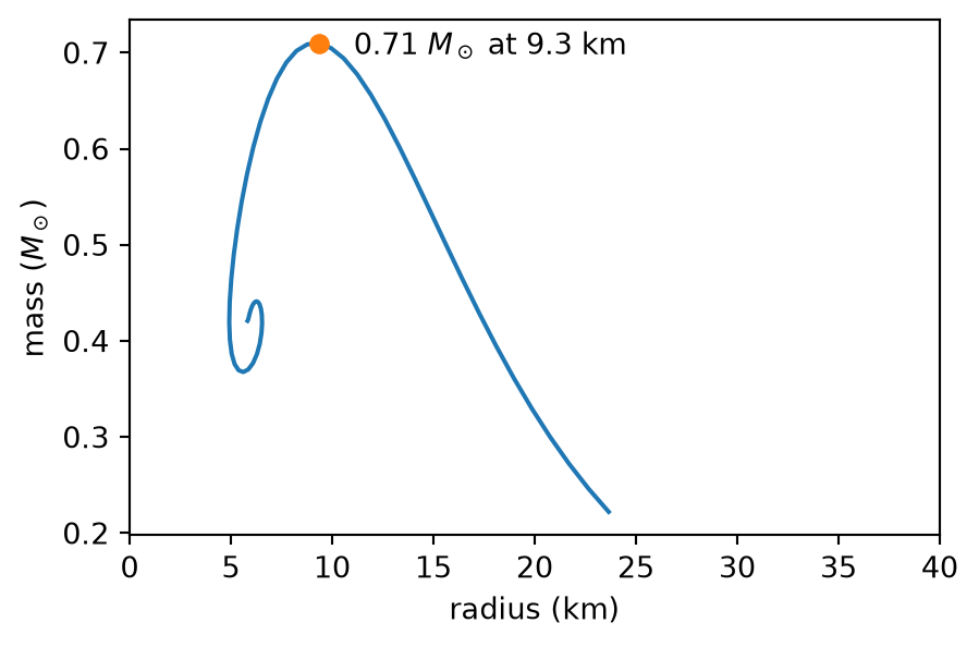

Figure 1: Mass against radius for stars of free neutrons, from integrating the TOV equation outward from the centre for a range of central densities. The maximum is the Oppenheimer–Volkoff limit.

The maximum in Figure 1 is a gravitational mass of 0.71 \(M_\odot\) at a radius of 9.3 km. Landau and Lifshitz (1980, sec. 109) quote \(0.76\,M_\odot\) at 9.4 km for the same model. Their figure is the rest mass \(N m_n\) of the neutrons, which exceeds the gravitational mass by the binding energy. Observed neutron stars reach about two solar masses, because nuclear forces stiffen the equation of state well beyond a free Fermi gas. The qualitative result stands: above some mass, no cold star can support itself.

Textbooks: Landau and Lifshitz (1975, sec. 100) set up the field equations inside matter, from which the TOV equation follows; Landau and Lifshitz (1980, secs. 106–109) cover dense matter and the neutron-star limit; Carroll (2004, sec. 5.8) derives the TOV equation. For the Newtonian version of the degeneracy argument, see the white dwarfs and the Chandrasekhar limit in Tong (n.d.-c, sec. 3.6.5).

6.3 Oppenheimer–Snyder collapse

Oppenheimer and Snyder (1939) took the simplest case, a uniform ball of pressureless dust starting from rest, and solved Einstein’s equations exactly. Outside the ball the metric is Schwarzschild’s, with gravitational radius \(r_g = 2GM/c^2\). Two results matter.

For an observer riding on the surface, the collapse takes a finite proper time, the same as Newtonian free fall from rest at radius \(R_0\): \[ \tau = \frac{\pi}{2}\sqrt{\frac{R_0^3}{2GM}}. \]

Code

R_sun = 6.957e8
tau_sun = np.pi / 2 * np.sqrt(R_sun**3 / (2 * G * M_sun))
r_g_sun = 2 * G * M_sun / c**2
print(f"tau = {tau_sun:.0f} s, r_g = {r_g_sun/1e3:.2f} km")

tau = 1769 s, r_g = 2.95 km

A ball with the Sun’s mass and radius would collapse in about 29 minutes of its own time, through a gravitational radius of 3.0 km.

For a distant observer, the surface never quite reaches \(r_g\). A radially falling surface obeys, in Schwarzschild time \(t\), \(\mathrm dr/\mathrm dt \to -c\,(1 - r_g/r)\) as \(r \to r_g\), so \[ r - r_g \propto \exp(-ct/r_g). \] The approach takes a time of order \(r_g/c\), tens of microseconds for a solar mass, after which light from the surface is redshifted beyond detection. Oppenheimer and Snyder put it as the star tending “to close itself off from any communication with a distant observer”. Landau and Lifshitz work through the same solution in modern coordinates (Landau and Lifshitz 1975, secs. 102–103).

Textbooks: besides Landau and Lifshitz (1975, secs. 102–103), Tong (2019, secs. 6.1.2–6.1.5) covers the horizon, the coordinates that cross it, and the formation of black holes by collapse, and Carroll (2004, secs. 5.6–5.8) does the same.

6.4 Why nobody followed it up

The paper describes what Wheeler named a black hole in 1967. The Ortega-Rodríguez et al. (2017) paper asks why it sat unused for two decades. One reason is on screen in the film’s Einstein scenes, though the film does not make the link: in October 1939 Einstein (1939) published a model of a cluster of particles in circular orbits and concluded that Schwarzschild singularities “do not exist in physical reality”. Oppenheimer himself never returned to the subject. Freeman Dyson called the collapse paper his one revolutionary contribution to science (Cho 2023).

7 January 1939: fission

The film shows Luis Alvarez reading about fission in a barber’s chair, rushing to tell Oppenheimer, and the oscilloscope that showed the ionisation pulses of fission fragments. Oppenheimer first says it can’t happen, then works out on the blackboard that it releases neutrons, and those neutrons could make a bomb.

7.1 The discovery

Hahn and Strassmann (1939) found barium among the products of uranium bombarded with neutrons. Meitner and Frisch (1939) explained it with Bohr’s liquid-drop model: the nucleus stretches and splits, and the two charged fragments fly apart. Frisch (1939) then saw the fragments’ ionisation pulses directly, the experiment Alvarez repeated at Berkeley.

7.2 How much energy

Meitner and Frisch estimated the energy two ways. The mass of a uranium nucleus exceeds that of the two fragments by about a fifth of a proton mass, about 200 MeV. Alternatively, two fragments of charge \(Ze/2\) touching each other carry Coulomb energy \[ E \approx \frac{(Z/2)^2 e^2}{4\pi\varepsilon_0 \cdot 2R_f},\qquad R_f = r_0 (A/2)^{1/3}. \]

Code

Z, A, r0 = 92, 236, 1.2e-15
R_f = r0 * (A / 2) ** (1 / 3)
E_touch = k_C * (Z / 2) ** 2 * e**2 / (2 * R_f) / MeV
print(f"two touching fragments: {E_touch:.0f} MeV")

two touching fragments: 259 MeV

This gives 259 MeV, an overestimate because real fragments are deformed and unequal, but the right size. A chemical reaction releases a few eV per molecule, so fission is about \(10^8\) times more energetic per event.

7.3 The liquid-drop barrier

Bohr and Wheeler (1939) made the model quantitative. In the semi-empirical mass formula the surface energy is \(E_S = a_s A^{2/3}\) and the Coulomb energy is \(E_C = a_c Z^2/A^{1/3}\). Stretch the sphere into a slight spheroid with deformation \(\alpha_2\); to second order \[ E_S(\alpha_2) = E_S\Bigl(1 + \tfrac{2}{5}\alpha_2^2\Bigr),\qquad E_C(\alpha_2) = E_C\Bigl(1 - \tfrac{1}{5}\alpha_2^2\Bigr). \] The surface resists deformation and the charge favours it. The sphere becomes unstable when \(E_C > 2E_S\), which defines the fissility \[ x = \frac{E_C}{2E_S} = \frac{a_c}{2a_s}\,\frac{Z^2}{A}. \]

Code

a_s, a_c = 17.8, 0.711   # MeV, one standard fit of the mass formula
Z2A_crit = 2 * a_s / a_c
x_U235 = 92**2 / 235 / Z2A_crit
print(f"(Z^2/A)_crit = {Z2A_crit:.1f}, U-235: Z^2/A = {92**2/235:.1f}, "
      f"x = {x_U235:.2f}")

(Z^2/A)_crit = 50.1, U-235: Z^2/A = 36.0, x = 0.72

The critical value of \(Z^2/A\) is about 50. Uranium has \(Z^2/A \approx 36\) and \(x \approx\) 0.72, so it sits behind a barrier of a few MeV. A neutron has to bring in enough energy to get over it.

7.4 Why only uranium-235

Bohr (1939) argued that slow neutrons split the rare isotope uranium-235, not the common uranium-238. The reason is pairing: nuclei with even numbers of neutrons are more tightly bound. A neutron joining uranium-235 makes even–even uranium-236 and releases its full binding energy. A neutron joining uranium-238 makes odd uranium-239 and releases less. The neutron separation energy is \(S_n(A{+}1) = [M(A) + m_n - M(A{+}1)]\,c^2\).

Code

S_n_236 = (mass["U235"] + mass["n"] - mass["U236"]) * u_MeV
S_n_239 = (mass["U238"] + mass["n"] - mass["U239"]) * u_MeV
print(f"S_n(U-236) = {S_n_236:.2f} MeV, S_n(U-239) = {S_n_239:.2f} MeV")

S_n(U-236) = 6.55 MeV, S_n(U-239) = 4.81 MeV

Capture by uranium-235 brings 6.5 MeV, above the fission barrier of about 6 MeV, so even a neutron at rest causes fission. Capture by uranium-238 brings only 4.8 MeV, so the neutron itself needs about a MeV of kinetic energy. Uranium-238 is 99.3% of natural uranium, and this is why the film’s Bohr tells Oppenheimer the whole country would have to become a factory.

Textbooks: Krane (1988) covers binding energies and the semi-empirical mass formula (§3.3), the liquid-drop barrier (§13.1) and the energy released (§13.3).

7.5 Secondary neutrons

The blackboard step in the film, from fission to a bomb, needs fission to release more neutrons than it absorbs. Three groups measured this within weeks in spring 1939 (Halban et al. 1939; Anderson et al. 1939; Szilard and Zinn 1939) and found two to three per fission.

Textbooks: Krane (1988, sec. 13.2), which also covers delayed neutrons.

8 Chain reactions and critical mass

8.1 Growth

If each fission produces \(\nu\) neutrons and each neutron causes another fission after a generation time \(\tau\), the number of neutrons grows as \[ N(t) = N_0 \exp\!\left(\frac{(\nu - 1)\,t}{\tau}\right) \quad\text{or, per generation,}\quad N_g = N_0\,\nu^{g}. \] For fast neutrons, \(\tau\) is the mean free path for fission divided by the neutron speed.

Code

rho_U = 18.71                          # g/cm^3, U-235 metal
n_U = rho_U / 235.04 * N_A             # nuclei per cm^3
sigma_f, sigma_el, nu = 1.235e-24, 4.566e-24, 2.637  # cm^2, 2 MeV neutrons
lam_f = 1 / (n_U * sigma_f)            # cm
lam_t = 1 / (n_U * (sigma_f + sigma_el))
v_n = np.sqrt(2 * 2 * MeV / m_n)       # m/s, 2 MeV neutron
tau_gen = lam_f / 100 / v_n            # s

nuclei_per_kg = 1000 / 235.04 * N_A
E_per_kg = nuclei_per_kg * 200 * MeV
gens = np.log(nuclei_per_kg) / np.log(nu)
print(f"lambda_f = {lam_f:.1f} cm, tau = {tau_gen*1e9:.1f} ns")
print(f"1 kg U-235: {E_per_kg:.2e} J = {E_per_kg/kt:.0f} kt; "
      f"{gens:.0f} generations = {gens*tau_gen*1e6:.2f} us")

lambda_f = 16.9 cm, tau = 8.6 ns
1 kg U-235: 8.21e+13 J = 20 kt; 58 generations = 0.50 us

With the cross-sections Reed (2021) uses for 2 MeV neutrons, a neutron travels about 17 cm between fissions, which takes 9 ns. Fissioning one kilogram of uranium-235 releases 82 TJ, about 20 kilotons of TNT, and takes about 58 generations from one neutron: half a microsecond. The bomb has to hold together for that long. Little Boy fissioned only about one kilogram of its 64 kg of uranium.

8.2 Critical size

Neutrons also leak out of the surface. In a sphere, production goes as the volume and leakage as the surface, so there is a critical radius. Treat the neutrons as diffusing with \(D = \lambda_t v/3\): \[ \frac{\partial n}{\partial t} = D\nabla^2 n + \frac{\nu - 1}{\tau}\,n . \] Separating variables, \(n = \mathrm e^{\alpha t}\sin(kr)/r\) with \(\alpha = (\nu-1)/\tau - Dk^2\). The sphere is critical when \(\alpha = 0\). If the density vanishes at the surface, \(kR = \pi\) and \[ R_c = \pi\sqrt{\frac{\lambda_t\lambda_f}{3(\nu - 1)}}. \] A better boundary condition lets neutrons escape freely, so the density falls to zero a distance beyond the surface. Reed (2021) uses \(n + \tfrac{2}{3}\lambda_t\,\mathrm dn/\mathrm dr = 0\) at \(r = R\).

Code

from scipy.optimize import brentq

k_c = np.sqrt(3 * (nu - 1) / (lam_t * lam_f))
R_naive = np.pi / k_c
bc = lambda R: (np.sin(k_c * R) / R + 2 / 3 * lam_t
                * (k_c * np.cos(k_c * R) / R - np.sin(k_c * R) / R**2))
R_crit = brentq(bc, 1, R_naive - 1e-9)
mass_kg = lambda R: 4 / 3 * np.pi * R**3 * rho_U / 1000
print(f"n = 0 at surface: R = {R_naive:.2f} cm, M = {mass_kg(R_naive):.0f} kg")
print(f"escape condition: R = {R_crit:.2f} cm, M = {mass_kg(R_crit):.1f} kg")

n = 0 at surface: R = 11.05 cm, M = 106 kg
escape condition: R = 8.37 cm, M = 45.9 kg

The crude boundary gives 11.0 cm and 106 kg. The escape condition gives 8.37 cm and 46 kg, Reed’s result, close to the measured bare critical mass of highly enriched uranium. Zorich (2015, sec. 5.6.3) builds a one-equation version of the same balance between production and leakage as an exercise in differential equations, and quotes 8.5 cm and about 50 kg.

8.3 Kilograms, not tons

Before 1940 most physicists assumed a bomb would need tons of uranium, because they thought of slow-neutron chains in natural uranium. The Frisch and Peierls (1940) memorandum asked about fast neutrons in pure uranium-235 and got an answer of the order of a kilogram. Their cross-section was too large and the answer far too small, but it moved the problem from impossible to industrial, and it started the British and then the American projects. Serber (1992) is the version the new arrivals at Los Alamos heard in April 1943. It adds the tamper, a heavy shell that reflects neutrons back and holds the core together a little longer, and the efficiency problem: the core blows itself apart after a few generations at most.

Textbooks: Krane (1988, sec. 13.9) on fission explosives, alongside Reed (2021).

9 Making the material: the marbles

The scene where Oppenheimer drops marbles into bowls, one for each month’s output of fissile material, is invented (Griffith 2023), but the arithmetic behind it is real. Natural uranium is 0.72% uranium-235. A bomb needs something like 80 to 90%.

9.1 Gaseous diffusion

Uranium hexafluoride molecules with the two isotopes have masses 349 and 352. At the same temperature, lighter molecules move faster and pass through a porous barrier slightly more often. Graham’s law gives the ideal separation factor per barrier: \[ \alpha = \sqrt{\frac{352}{349}}. \]

Code

alpha = np.sqrt(352 / 349)
x_f, x_p = 0.0072, 0.90
ratio = np.log((x_p / (1 - x_p)) / (x_f / (1 - x_f)))
stages = ratio / np.log(np.sqrt(alpha))
print(f"alpha = {alpha:.5f}; stages at sqrt(alpha) each: {stages:.0f}")

alpha = 1.00429; stages at sqrt(alpha) each: 3329

That is \(\alpha =\) 1.0043, a change of 0.4% per pass. In an ideal cascade each stage raises the abundance ratio \(x/(1-x)\) by about \(\sqrt\alpha\), so going from 0.72% to 90% takes about 3,300 stages. That is why the K-25 plant at Oak Ridge was one of the largest buildings in the world.

Textbooks: Lifshitz and Pitaevskii (1981, sec. 15) derive the flow of a rarefied gas through a small hole: the mass leaving per unit time is \(Q = sP\sqrt{m/2\pi T}\) (temperature in energy units), so the number of molecules goes as \(1/\sqrt m\), which is Graham’s law.

9.2 Calutrons

Lawrence’s alternative was a mass spectrometer on an industrial scale. An ion of charge \(q\) accelerated through voltage \(V\) moves on a circle of radius \[ r = \frac{1}{B}\sqrt{\frac{2mV}{q}}, \qquad \frac{\Delta r}{r} = \frac{\Delta m}{2m} = \frac{3}{2 \times 238} \approx 0.6\%. \] After half a turn the two beams land \(2\,\Delta r\) apart: about 1.5 cm for a radius of about 1.2 m. Space charge and beam spread made it far harder than this suggests.

9.3 Plutonium

The other route makes a new fissile element in a reactor: \[ {}^{238}\mathrm U + n \to {}^{239}\mathrm U \xrightarrow{\beta^-,\ 23.5\ \text{min}} {}^{239}\mathrm{Np} \xrightarrow{\beta^-,\ 2.36\ \text{d}} {}^{239}\mathrm{Pu}. \] McMillan and Abelson (1940) published the first step in open literature. The discovery of plutonium (Seaborg et al. 1946) and its fissility (Kennedy et al. 1946) were held back until 1946.

9.4 Fermi’s pile

Chicago Pile-1 went critical on 2 December 1942; the film mentions it only in passing. A reactor can be controlled at all because about 0.65% of the neutrons from uranium-235 fission come out seconds later, from decaying fission fragments. With a small excess reactivity \(k - 1\), the power grows with period \[ T \approx \frac{\ell_{\text{eff}}}{k - 1}, \] where \(\ell_{\text{eff}}\) is the mean neutron lifetime including the delayed ones, about a tenth of a second. Prompt neutrons alone, with lifetimes of a millisecond in graphite, would give periods too short for any control rod.

Textbooks: Krane (1988, secs. 13.5–13.6), which builds the multiplication factor of a pile like Fermi’s from the four-factor formula.

10 Igniting the atmosphere

The film’s tensest physics is Teller’s worry that the bomb’s heat could start a self-sustaining fusion reaction in the air, and Oppenheimer’s “near zero”. The analysis that settled it is Konopinski et al. (1946), written up in 1946 from wartime work. The reaction they feared most was \[ {}^{14}\mathrm N + {}^{14}\mathrm N \to {}^{24}\mathrm{Mg} + {}^4\mathrm{He}. \]

Code

Q_NN = (2 * mass["N14"] - mass["Mg24"] - mass["He4"]) * u_MeV
R_NN = 1.2e-15 * 2 * 14 ** (1 / 3)
V_NN = k_C * 7 * 7 * e**2 / R_NN / MeV
print(f"Q = {Q_NN:.1f} MeV, Coulomb barrier = {V_NN:.0f} MeV")

Q = 17.2 MeV, Coulomb barrier = 12 MeV

The reaction releases 17.2 MeV, but two nitrogen nuclei must climb a Coulomb barrier of about 12 MeV, so the rate at any plausible temperature depends on tunnelling deep under it. The argument in LA-602 compares rates. At temperature \(T\) the reaction heats the air at a rate set by the tunnelling probability, and the air cools by radiation and by Compton scattering of its electrons on the radiation. A reaction spreads only if \[ \frac{\mathrm d E_{\text{fusion}}}{\mathrm dt} > \frac{\mathrm d E_{\text{radiation}}}{\mathrm dt} \] everywhere along the front. They found the losses ahead at every temperature, by a margin that survived pessimistic choices of every cross-section.

The history is thinner than the film suggests. Teller raised the idea at Oppenheimer’s Berkeley summer study in 1942 and Bethe dismissed it within days (Rhodes 1986; Griffith 2023). Oppenheimer discussed it with Compton, not Einstein (Greenberg and Tuquero 2023).

Textbooks: the Coulomb-barrier tunnelling factor is in Landau and Lifshitz (1977, sec. 50, Problem 2), and Krane (1988, secs. 14.1–14.2) applies it to fusion rates. The losses LA-602 weighed against it are bremsstrahlung from electrons scattering off nuclei and Compton scattering, both in Berestetskii et al. (1982, sec. 92 and §86).

11 Plutonium and implosion

11.1 Why the gun fails for plutonium

Reactor plutonium contains some plutonium-240, which fissions spontaneously and emits neutrons. A gun brings two subcritical pieces together at a few hundred metres per second, so assembly takes a fraction of a millisecond. A stray neutron in that window starts the chain early, in a barely critical configuration, and the bomb fizzles.

Code

core_g, f_240, sf_rate = 6200, 0.01, 1000   # g, mass fraction, n/(g s)
t_assemble = 0.1 / 300                      # s: 10 cm at 300 m/s
n_source = core_g * f_240 * sf_rate
print(f"{n_source:.0f} neutrons/s, {n_source * t_assemble:.0f} "
      f"during assembly")

62000 neutrons/s, 21 during assembly

With illustrative values (a 6.2 kg core, 1% plutonium-240 emitting about 1000 neutrons per gram per second, 10 cm closed at 300 m/s), about 21 neutrons appear during assembly. Predetonation is close to certain. Segrè’s measurements of reactor plutonium in 1944 showed this, and Los Alamos dropped the plutonium gun (Hoddeson et al. 1993).

11.2 Implosion

Implosion assembles the core in microseconds by crushing it. Compression also lowers the critical mass. Both mean free paths scale as \(1/\rho\), so \(R_c \propto 1/\rho\) and \[ M_c = \tfrac{4}{3}\pi R_c^3 \rho \propto \frac{1}{\rho^2}. \] Doubling the density cuts the critical mass by four. The film credits Seth Neddermeyer with the idea. Making it work needed explosive lenses to shape a converging spherical shock, the problem George Kistiakowsky’s division solved; Hoddeson et al. (1993) is the detailed account.

12 Trinity

12.1 The delay

The film’s sound arrives well after the flash, which several reviewers checked (Virginia Tech News 2023; Griffith 2023). Sound in air travels at about 343 m/s:

Code

for miles in (6, 10):
    print(f"{miles} miles: {miles * 1609.34 / 343:.0f} s")

6 miles: 28 s
10 miles: 47 s

12.2 Fermi’s paper strips

Fermi dropped scraps of paper as the blast wave passed base camp, about 16 km away, measured how far it moved them, and estimated the yield on the spot. His memorandum records a displacement of about 2.5 m and an estimate of about ten kilotons (Fermi 1945).

12.3 Taylor’s dimensional analysis

In 1950 G. I. Taylor published the theory of a point explosion in air (Taylor 1950a) and applied it to photographs of the Trinity fireball that had been released in 1947 (Taylor 1950b). If a large energy \(E\) is released at a point in gas of density \(\rho_0\), at early times the shock radius can depend only on \(E\), \(\rho_0\) and \(t\). The only combination with the dimension of length is \[ R(t) = S(\gamma)\left(\frac{E\,t^2}{\rho_0}\right)^{1/5}, \] where Taylor found \(S \approx 1.03\) for air with \(\gamma = 1.4\). Plotting \(\log R\) against \(\log t\) should give a line of slope \(2/5\), and its intercept gives \(E\).

Code

trinity = np.array([  # t (ms), R (m), from Taylor (1950b)
    [0.10, 11.1], [0.24, 19.9], [0.38, 25.4], [0.52, 28.8], [0.66, 31.9],
    [0.80, 34.2], [0.94, 36.3], [1.08, 38.9], [1.22, 41.0], [1.36, 42.8],
    [1.50, 44.4], [1.65, 46.0], [1.79, 46.9], [1.93, 48.7], [3.26, 59.0],
    [3.53, 61.1], [3.80, 62.9], [4.07, 64.3], [4.34, 65.6], [4.61, 67.3],
    [15.0, 106.5], [25.0, 130.0], [34.0, 145.0], [53.0, 175.0],
    [62.0, 185.0]])
t_s, R_m = trinity[:, 0] / 1e3, trinity[:, 1]
slope, _ = np.polyfit(np.log(t_s), np.log(R_m), 1)
log_c = np.mean(np.log(R_m) - 0.4 * np.log(t_s))   # fix the slope at 2/5
rho_air, S_gamma = 1.25, 1.033
E_taylor = rho_air * np.exp(5 * log_c) / S_gamma**5

fig, ax = plt.subplots(figsize=(5, 3.2))
ax.loglog(t_s * 1e3, R_m, "o", ms=4, label="Taylor's data")
tt = np.logspace(-4.1, -1.1, 50)
ax.loglog(tt * 1e3, np.exp(log_c) * tt**0.4, label="slope 2/5")
ax.set_xlabel("t (ms)")
ax.set_ylabel("R (m)")
ax.legend()
plt.show()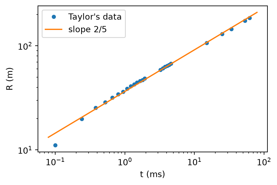

Figure 2: Radius of the Trinity shock front against time, from the photographs in Taylor (1950b), with the fitted line of slope 2/5.

The free fit has slope 0.406, close to 0.4. With the slope fixed at 2/5, \(\rho_0 = 1.25\) kg/m³ and \(S = 1.033\), the energy is 68 TJ, about 16 kilotons. Taylor’s own figure was close to this. The yield was still secret when he published, and the official figure today is about 21 kilotons. Rabi’s guess of 18 kilotons, which won the film’s betting pool, was closer than either estimate.

Landau and Lifshitz (1987, sec. 106) derive the full self-similar solution, which gives \(S(\gamma)\). They credit it to Sedov (1946) and von Neumann (1947), and note that Taylor’s treatment, written in 1941 and published in 1950, stopped short of an analytic solution.

13 The Super

The last act turns on the hydrogen bomb. The reaction that matters is deuterium–tritium fusion: \[ {}^2\mathrm H + {}^3\mathrm H \to {}^4\mathrm{He} + n. \]

Code

Q_DT = (mass["H2"] + mass["H3"] - mass["He4"] - mass["n"]) * u_MeV
print(f"Q = {Q_DT:.1f} MeV")

Q = 17.6 MeV

It releases 17.6 MeV, and the Coulomb barrier between two charges of one is low enough for it to run at temperatures a fission bomb can reach. Teller’s wartime design, the “classical Super”, tried to start a burning wave in a cylinder of deuterium with a fission trigger. Calculations in 1950 showed the wave would die out. The Teller–Ulam idea of 1951 used radiation from the fission stage to compress the fusion fuel first, the same lesson as implosion at a different scale. This is where the open literature stops: the reports remain partly classified, and the film keeps this part of the story to politics. The General Advisory Committee report of October 1949, which Oppenheimer chaired and which opposed a crash programme, is the document behind the security hearing scenes; Bird and Sherwin (2005) and Wellerstein (2021) cover it.

Textbooks: Krane (1988, sec. 14.5).

14 Scene index

Scene	Physics	Sources
Göttingen with Born	Molecules: separating electron and nuclear motion	Born and Oppenheimer (1927); Oppenheimer (1927)
Heisenberg lecturing	Uncertainty	Heisenberg (1927); Kennard (1927)
Teaching at Berkeley	Tunnelling, the anti-electron, deuteron reactions	Oppenheimer (1928); Oppenheimer (1930); Oppenheimer and Phillips (1935)
Lawrence’s Radiation Laboratory	Cyclotron, later calutrons	Lawrence and Livingston (1932)
Snyder and the collapsing star	Neutron-star limit, gravitational collapse	Oppenheimer and Volkoff (1939); Oppenheimer and Snyder (1939); Ortega-Rodríguez et al. (2017)
Einstein at Princeton	Einstein’s rejection of collapse	Einstein (1939)
Alvarez in the barber’s chair, the oscilloscope	Fission	Hahn and Strassmann (1939); Meitner and Frisch (1939); Frisch (1939)
Bohr on turning the country into a factory	Uranium-235 only	Bohr (1939); Bohr and Wheeler (1939)
Recruiting for Los Alamos, first lectures	Critical mass, tamper, efficiency	Frisch and Peierls (1940); Serber (1992); Reed (2021)
The marbles in bowls	Isotope separation, plutonium production	Smyth (1945); Reed (2021)
Teller’s ignition calculation, “near zero”	Nitrogen fusion versus radiation losses	Konopinski et al. (1946)
Neddermeyer and implosion	Predetonation, \(M_c \propto \rho^{-2}\)	Hoddeson et al. (1993)
Trinity: delay, betting pool	Blast scaling, yield	Fermi (1945); Taylor (1950b)
The Super and the hearing	D–T fusion, secrecy	Wellerstein (2021); Bird and Sherwin (2005)

15 Reading list

For the film itself, Griffith (2023) and Whitfield (2024). For the life, Bird and Sherwin (2005), which the film adapts. For the history of the project, Rhodes (1986). For the physics of the bomb, Reed (2021), with Serber (1992) as the primary source and Hoddeson et al. (1993) for what Los Alamos actually did. For secrecy and what it did to the literature, Wellerstein (2021). For the astrophysics, Oppenheimer and Snyder (1939) is five pages and readable today, Ortega-Rodríguez et al. (2017) explains its neglect, and Landau and Lifshitz (1975, secs. 102–103) and Landau and Lifshitz (1980, sec. 109) give the textbook treatment.

Most sections end with textbook references. Landau and Lifshitz are the classic treatment. David Tong’s Cambridge lecture notes are free online, so every reader can follow those. Shankar (1994) and Carroll (2004) are the standard modern texts for quantum mechanics and general relativity, and Krane (1988) for the nuclear physics.

References

Anderson, Carl D. 1933. “The Positive Electron.” Physical Review 43 (6): 491–94. https://doi.org/10.1103/PhysRev.43.491.

Anderson, H. L., E. Fermi, and H. B. Hanstein. 1939. “Production of Neutrons in Uranium Bombarded by Neutrons.” Physical Review 55: 797–98. https://doi.org/10.1103/PhysRev.55.797.2.

ANSTO. 2023. “ANSTO Scientists Would Have Preferred More about the Physics but Impressed with Oppenheimer.” https://www.ansto.gov.au/news/ansto-scientists-would-have-preferred-more-about-physics-but-impressed-oppenheimer.

Berestetskii, V. B., E. M. Lifshitz, and L. P. Pitaevskii. 1982. Quantum Electrodynamics. 2nd ed. Vol. 4. Course of Theoretical Physics. Pergamon.

Bird, Kai, and Martin J. Sherwin. 2005. American Prometheus: The Triumph and Tragedy of J. Robert Oppenheimer. Knopf.

Bohr, N. 1939. “Resonance in Uranium and Thorium Disintegrations and the Phenomenon of Nuclear Fission.” Physical Review 55: 418–19. https://doi.org/10.1103/PhysRev.55.418.2.

Bohr, N., and J. A. Wheeler. 1939. “The Mechanism of Nuclear Fission.” Physical Review 56: 426–50. https://doi.org/10.1103/PhysRev.56.426.

Born, M., and R. Oppenheimer. 1927. “Zur Quantentheorie Der Molekeln.” Annalen Der Physik 389 (20): 457–84. https://doi.org/10.1002/andp.19273892002.

Carroll, Sean M. 2004. Spacetime and Geometry: An Introduction to General Relativity. Addison Wesley.

Cho, Adrian. 2023. “Hollywood Movie Aside, Just How Good a Physicist Was Oppenheimer?” Science, July 17.

Dirac, P. A. M. 1931. “Quantised Singularities in the Electromagnetic Field.” Proceedings of the Royal Society of London A 133 (821): 60–72. https://doi.org/10.1098/rspa.1931.0130.

Durrani, Matin, James Dacey, Hamish Johnston, Michael Banks, and Kate Gardner. 2023. “Oppenheimer the Movie: Physics World Writers Give Their Verdict.” Physics World. https://physicsworld.com/a/oppenheimer-the-movie-physics-world-writers-give-their-verdict/.

Einstein, Albert. 1939. “On a Stationary System with Spherical Symmetry Consisting of Many Gravitating Masses.” Annals of Mathematics 40 (4): 922–36. https://doi.org/10.2307/1968902.

Fermi, Enrico. 1945. My Observations During the Explosion at Trinity on July 16, 1945. https://fermatslibrary.com/s/my-observations-during-the-explosion-at-trinity.

Flerov, G. N., and K. A. Petrjak. 1940. “Spontaneous Fission of Uranium.” Physical Review 58: 89. https://doi.org/10.1103/PhysRev.58.89.2.

Frisch, O. R. 1939. “Physical Evidence for the Division of Heavy Nuclei Under Neutron Bombardment.” Nature 143: 276. https://doi.org/10.1038/143276a0.

Frisch, Otto R., and Rudolf Peierls. 1940. On the Construction of a “Super-Bomb”; Based on a Nuclear Chain Reaction in Uranium.

Greenberg, Jon, and Loreben Tuquero. 2023. “MovieFact: ‘Oppenheimer’ Sticks Close to Historic Record, with Some Liberties.” PolitiFact, August 25. https://www.politifact.com/article/2023/aug/25/movie-oppenheimer-fact-check-historical-real/.

Griffith, Chris. 2023. “A Manhattan Project Historian Comments on ‘Oppenheimer’.” Bulletin of the Atomic Scientists, July 28. https://thebulletin.org/2023/07/a-manhattan-project-historian-comments-on-oppenheimer/.

Hahn, O., and F. Strassmann. 1939. “Über Den Nachweis Und Das Verhalten Der Bei Der Bestrahlung Des Urans Mittels Neutronen Entstehenden Erdalkalimetalle.” Die Naturwissenschaften 27: 11–15. https://doi.org/10.1007/BF01488241.

Halban, H. von, F. Joliot, and L. Kowarski. 1939. “Liberation of Neutrons in the Nuclear Explosion of Uranium.” Nature 143 (3620): 470–71. https://doi.org/10.1038/143470a0.

Heisenberg, W. 1927. “Über Den Anschaulichen Inhalt Der Quantentheoretischen Kinematik Und Mechanik.” Zeitschrift für Physik 43: 172–98. https://doi.org/10.1007/BF01397280.

Hoddeson, Lillian, Paul W. Henriksen, Roger A. Meade, and Catherine Westfall. 1993. Critical Assembly: A Technical History of Los Alamos During the Oppenheimer Years, 1943–1945. Cambridge University Press. https://doi.org/10.1017/CBO9780511665400.

Kennard, E. H. 1927. “Zur Quantenmechanik Einfacher Bewegungstypen.” Zeitschrift für Physik 44: 326–52. https://doi.org/10.1007/BF01391200.

Kennedy, J. W., G. T. Seaborg, E. Segrè, and A. C. Wahl. 1946. “Properties of 94(239).” Physical Review 70: 555–56. https://doi.org/10.1103/PhysRev.70.555.

Konopinski, E. J., C. Marvin, and E. Teller. 1946. Ignition of the Atmosphere with Nuclear Bombs. Report LA-602. Los Alamos Laboratory.

Krane, Kenneth S. 1988. Introductory Nuclear Physics. Wiley.

Landau, L. 1938. “Origin of Stellar Energy.” Nature 141 (3564): 333–34. https://doi.org/10.1038/141333b0.

Landau, L. D., and E. M. Lifshitz. 1975. The Classical Theory of Fields. 4th ed. Vol. 2. Course of Theoretical Physics. Pergamon.

Landau, L. D., and E. M. Lifshitz. 1977. Quantum Mechanics: Non-Relativistic Theory. 3rd ed. Vol. 3. Course of Theoretical Physics. Pergamon.

Landau, L. D., and E. M. Lifshitz. 1980. Statistical Physics, Part 1. 3rd ed. Vol. 5. Course of Theoretical Physics. Pergamon.

Landau, L. D., and E. M. Lifshitz. 1987. Fluid Mechanics. 2nd ed. Vol. 6. Course of Theoretical Physics. Pergamon.

Lawrence, Ernest O., and M. Stanley Livingston. 1932. “The Production of High Speed Light Ions Without the Use of High Voltages.” Physical Review 40: 19–35. https://doi.org/10.1103/PhysRev.40.19.

Lifshitz, E. M., and L. P. Pitaevskii. 1981. Physical Kinetics. Vol. 10. Course of Theoretical Physics. Pergamon.

Los Alamos National Laboratory. 2023. “Oppenheimer’s Scientific Contributions.” National Security Science, July. https://lanl.gov/media/publications/national-security-science/0723-oppenheimers-scientific-contributions.

McMillan, Edwin, and Philip Hauge Abelson. 1940. “Radioactive Element 93.” Physical Review 57: 1185–86. https://doi.org/10.1103/PhysRev.57.1185.2.

Meitner, Lise, and O. R. Frisch. 1939. “Disintegration of Uranium by Neutrons: A New Type of Nuclear Reaction.” Nature 143: 239–40. https://doi.org/10.1038/143239a0.

Oppenheimer, J. R. 1927. “Zur Quantentheorie Kontinuierlicher Spektren.” Zeitschrift für Physik 41: 268–93. https://doi.org/10.1007/BF01391242.

Oppenheimer, J. R. 1928. “Three Notes on the Quantum Theory of Aperiodic Effects.” Physical Review 31 (1): 66–81. https://doi.org/10.1103/PhysRev.31.66.

Oppenheimer, J. R. 1930. “On the Theory of Electrons and Protons.” Physical Review 35: 562–63. https://doi.org/10.1103/PhysRev.35.562.

Oppenheimer, J. R., and M. Phillips. 1935. “Note on the Transmutation Function for Deuterons.” Physical Review 48: 500–502. https://doi.org/10.1103/PhysRev.48.500.

Oppenheimer, J. R., and Robert Serber. 1938. “On the Stability of Stellar Neutron Cores.” Physical Review 54 (7): 540. https://doi.org/10.1103/PhysRev.54.540.

Oppenheimer, J. R., and H. Snyder. 1939. “On Continued Gravitational Contraction.” Physical Review 56: 455–59. https://doi.org/10.1103/PhysRev.56.455.

Oppenheimer, J. R., and G. M. Volkoff. 1939. “On Massive Neutron Cores.” Physical Review 55: 374–81. https://doi.org/10.1103/PhysRev.55.374.

Ortega-Rodríguez, Manuel, Hugo Solís-Sánchez, Eduardo Boza-Oviedo, et al. 2017. “The Early Scientific Contributions of J. Robert Oppenheimer: Why Did the Scientific Community Miss the Black Hole Opportunity?” Physics in Perspective 19: 60–75. https://doi.org/10.1007/s00016-017-0195-6.

Reed, B. Cameron. 2021. The Physics of the Manhattan Project. 4th ed. Springer. https://doi.org/10.1007/978-3-030-61373-0.

Reed, B. Cameron. 2024. “Defending Oppenheimer.” Physics Today 77 (10): 11. https://doi.org/10.1063/pt.mruy.bkwf.

Rhodes, Richard. 1986. The Making of the Atomic Bomb. Simon & Schuster.

Santiago, Bárbara Cruvinel, and Lindsay Rand. 2024. “Beyond the Cinematic Feat: Consequences Oppenheimer Ignored.” Physics Today 77 (7): 11. https://doi.org/10.1063/pt.xasn.zlyg.

Seaborg, G. T., E. M. McMillan, J. W. Kennedy, and A. C. Wahl. 1946. “Radioactive Element 94 from Deuterons on Uranium.” Physical Review 69: 366–67. https://doi.org/10.1103/PhysRev.69.366.2.

Serber, Robert. 1992. The Los Alamos Primer: The First Lectures on How to Build an Atomic Bomb. University of California Press.

Shankar, R. 1994. Principles of Quantum Mechanics. 2nd ed. Plenum.

Smyth, Henry DeWolf. 1945. Atomic Energy for Military Purposes. Princeton University Press.

Szilard, Leo, and Walter H. Zinn. 1939. “Instantaneous Emission of Fast Neutrons in the Interaction of Slow Neutrons with Uranium.” Physical Review 55: 799–800. https://doi.org/10.1103/PhysRev.55.799.

Taylor, Geoffrey. 1950a. “The Formation of a Blast Wave by a Very Intense Explosion I. Theoretical Discussion.” Proceedings of the Royal Society of London A 201: 159–74. https://doi.org/10.1098/rspa.1950.0049.

Taylor, Geoffrey. 1950b. “The Formation of a Blast Wave by a Very Intense Explosion II. The Atomic Explosion of 1945.” Proceedings of the Royal Society of London A 201: 175–86. https://doi.org/10.1098/rspa.1950.0050.

Tolman, Richard C. 1939. “Static Solutions of Einstein’s Field Equations for Spheres of Fluid.” Physical Review 55: 364–73. https://doi.org/10.1103/PhysRev.55.364.

Tong, David. 2006. “Quantum Field Theory.” https://davidtong.org/teaching/quantum-field-theory/.

Tong, David. 2013. “Dynamics and Relativity.” https://davidtong.org/teaching/dynamics-and-relativity/.

Tong, David. 2017. “Topics in Quantum Mechanics.” https://davidtong.org/teaching/topics-in-quantum-mechanics/.

Tong, David. 2019. “General Relativity.” https://davidtong.org/teaching/general-relativity/.

Tong, David. n.d.-a. “Particle Physics.” https://davidtong.org/teaching/particle-physics/.

Tong, David. n.d.-b. “Quantum Mechanics.” https://davidtong.org/teaching/quantum-mechanics/.

Tong, David. n.d.-c. “Statistical Physics.” https://davidtong.org/teaching/statistical-physics/.

Virginia Tech News. 2023. “Virginia Tech Particle Physicist: Christopher Nolan’s ‘Oppenheimer’ Film Excels at Accuracy.” July. https://news.vt.edu/articles/2023/07/science-pitts-oppenheimer-film-facts.html.

Wellerstein, Alex. 2021. Restricted Data: The History of Nuclear Secrecy in the United States. University of Chicago Press. https://doi.org/10.7208/chicago/9780226020419.001.0001.

Whitfield, Stephen J. 2024. “Oppenheimer.” Journal of American History 111 (1): 200–203. https://doi.org/10.1093/jahist/jaae084.

Zorich, Vladimir A. 2015. Mathematical Analysis I. 2nd ed. Universitext. Springer. https://doi.org/10.1007/978-3-662-48792-1.