Numerical

plotdf (dydx, options…) — Function

The function plotdf creates a two-dimensional plot of the direction field (also called slope field) for a first-order Ordinary Differential Equation (ODE) or a system of two autonomous first-order ODE’s.

Plotdf requires Xmaxima, even if its run from a Maxima session in a console, since the plot will be created by the Tk scripts in Xmaxima. If Xmaxima is not installed plotdf will not work.

dydx, dxdt and dydt are expressions that depend on x and y. dvdu, dudt and dvdt are expressions that depend on u and v. In addition to those two variables, the expressions can also depend on a set of parameters, with numerical values given with the parameters option (the option syntax is given below), or with a range of allowed values specified by a sliders option.

Several other options can be given within the command, or selected in the menu. Integral curves can be obtained by clicking on the plot, or with the option trajectory_at. The direction of the integration can be controlled with the direction option, which can have values of forward, backward or both. The number of integration steps is given by nsteps; at each integration step the time increment will be adjusted automatically to produce displacements much smaller than the size of the plot window. The numerical method used is 4th order Runge-Kutta with variable time steps.

Plot window menu:

The menu bar of the plot window has the following five buttons:

Close: can be used to close the plot window.

Config: opens the configuration menu with several fields that show the ODE(s) in use and various other settings. If a pair of coordinates are entered in the field Trajectory at and the enter key is pressed, a new integral curve will be shown, in addition to the ones already shown.

Save: used to save a copy of the plot, in Postscript format, in the file specified in a field of the window that appears when that button is clicked.

Replot: replots the direction field with the new settings defined in the configuration menu and replots only the last integral curve that was previously plotted. If you just resized the plot window, the size and width of the arrows and curves will be adapted to the new size if you click on Replot.

Time plot: creates two new window showing the plots of the two variables in terms of time, for the last integral curve that was plotted.

Plot options:

Options can also be given within the plotdf itself, each one being a list of two or more elements. The first element in each option is the name of the option, and the remainder is the value or values assigned to the option.

The options which are recognized by plotdf are the following:

nsteps defines the number of steps that will be used for the independent variable, to compute an integral curve. The default value is 100.

direction defines the direction of the independent variable that will be followed to compute an integral curve. Possible values are forward, to make the independent variable increase nsteps times, with increments tstep, backward, to make the independent variable decrease, or both that will lead to an integral curve that extends nsteps forward, and nsteps backward. The keywords right and left can be used as synonyms for forward and backward. The default value is both.

tinitial defines the initial value of variable t used to compute integral curves. Since the differential equations are autonomous, that setting will only appear in the plot of the curves as functions of t. The default value is 0.

versus_t is used to create a second plot window, with a plot of an integral curve, as two functions x, y, of the independent variable t. If versus_t is given any value different from 0, the second plot window will be displayed. The second plot window includes another menu, similar to the menu of the main plot window. The default value is 0.

trajectory_at defines the coordinates xinitial and yinitial for the starting point of an integral curve. The option is empty by default.

parameters defines a list of parameters, and their numerical values, used in the definition of the differential equations. The name and values of the parameters must be given in a string with a comma-separated sequence of pairs name=value.

sliders defines a list of parameters that will be changed interactively using slider buttons, and the range of variation of those parameters. The names and ranges of the parameters must be given in a string with a comma-separated sequence of elements name=min:max

tstep sets the value of the time intervals used in the integration algorithm. It must be a floating point number; you might have to adjust its value to get good results for the integral curves. If not given, a default value will be chosen according to the region to be plotted.

xfun defines a string with semi-colon-separated sequence of functions of x to be displayed, on top of the direction field. Those functions will be parsed by Tcl and not by Maxima.

x should be followed by two numbers, which will set up the minimum and maximum values shown on the horizontal axis. If the variable on the horizontal axis is not x, then this option should have the name of the variable on the horizontal axis. The default horizontal range is from -10 to 10.

y should be followed by two numbers, which will set up the minimum and maximum values shown on the vertical axis. If the variable on the vertical axis is not y, then this option should have the name of the variable on the vertical axis. The default vertical range is from -10 to 10.

xaxislabel will be used to identify the horizontal axis. Its default value is the name of the first state variable.

yaxislabel will be used to identify the vertical axis. Its default value is the name of the second state variable.

number_of_arrows should be set to a square number and defines the approximate density of the arrows being drawn. The default value is 225.

Examples:

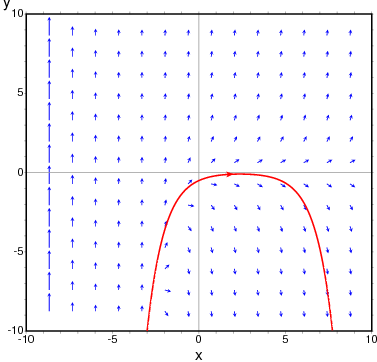
To show the direction field of the differential equation $y’ = e^{-x} + y$ and the solution that goes through $(2, -0.1)$:

maxima
(%i1) plotdf(exp(-x)+y,[trajectory_at,2,-0.1])$

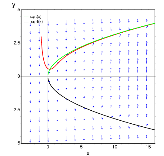
To obtain the direction field for the equation $dy/dx = x - y^2$

and the solution with initial condition $y(-1) = 3$, we can use the command:

maxima
(%i1) plotdf(x-y^2,[xfun,"sqrt(x);-sqrt(x)"],
         [trajectory_at,-1,3], [direction,forward],
         [y,-5,5], [x,-4,16])$

The graph also shows the function $y = \sqrt{x}.$

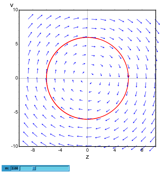
The following example shows the direction field of a harmonic oscillator, defined by the two equations $dz/dt = v$ and $dv/dt = -kz/m,$

and the integral curve through $(z,v) = (6,0)$, with a slider that will allow you to change the value of $m$ interactively ($k$ is fixed at 2):

maxima
(%i1) plotdf([v,-k*z/m], [z,v], [parameters,"m=2,k=2"],
           [sliders,"m=1:5"], [trajectory_at,6,0])$

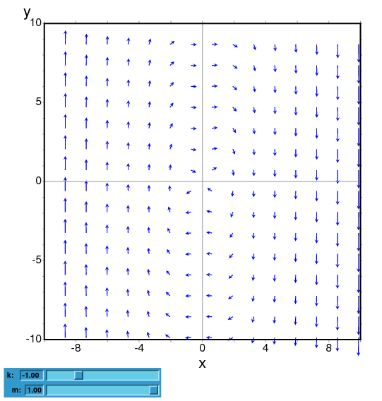
To plot the direction field of the Duffing equation, $m x’‘+c x’ + kx + bx^3 = 0,$ we introduce the variable $y=x’$ and use:

maxima
(%i1) plotdf([y,-(k*x + c*y + b*x^3)/m],
             [parameters,"k=-1,m=1.0,c=0,b=1"],
             [sliders,"k=-2:2,m=-1:1"],[tstep,0.1])$

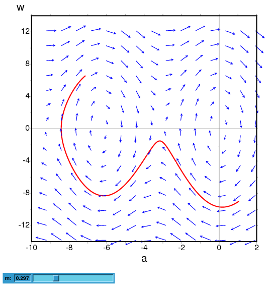
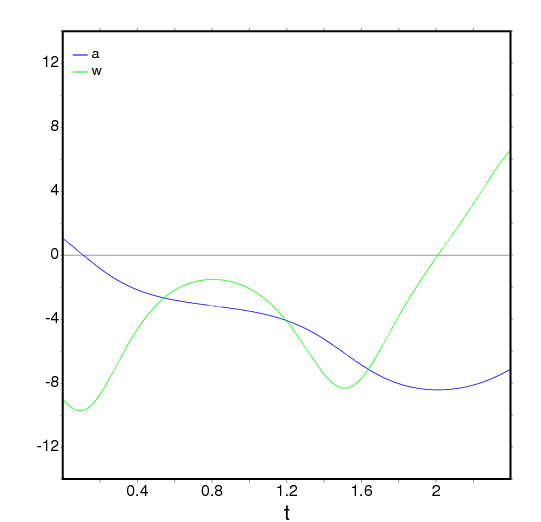
The direction field for a damped pendulum, including the solution for the given initial conditions, with a slider that can be used to change the value of the mass $m$, and with a plot of the two state variables as a function of time:

maxima
(%i1) plotdf([w,-g*sin(a)/l - b*w/m/l], [a,w],
        [parameters,"g=9.8,l=0.5,m=0.3,b=0.05"],
        [trajectory_at,1.05,-9],[tstep,0.01],
        [a,-10,2], [w,-14,14], [direction,forward],
        [nsteps,300], [sliders,"m=0.1:1"], [versus_t,1])$

ploteq (exp, …options…) — Function

Plots equipotential curves for exp, which should be an expression depending on two variables. The curves are obtained by integrating the differential equation that define the orthogonal trajectories to the solutions of the autonomous system obtained from the gradient of the expression given. The plot can also show the integral curves for that gradient system (option fieldlines).

This program also requires Xmaxima, even if its run from a Maxima session in a console, since the plot will be created by the Tk scripts in Xmaxima. By default, the plot region will be empty until the user clicks in a point (or gives its coordinate with in the set-up menu or via the trajectory_at option).

Most options accepted by plotdf can also be used for ploteq and the plot interface is the same that was described in plotdf.

Example:

maxima
(%i1) V: 900/((x+1)^2+y^2)^(1/2)-900/((x-1)^2+y^2)^(1/2)$
(%i2) ploteq(V,[x,-2,2],[y,-2,2],[fieldlines,"blue"])$

Clicking on a point will plot the equipotential curve that passes by that point (in red) and the orthogonal trajectory (in blue).

rk (ODE, var, initial, domain) — Function

The first form solves numerically one first-order ordinary differential equation, and the second form solves a system of m of those equations, using the 4th order Runge-Kutta method. var represents the dependent variable. ODE must be an expression that depends only on the independent and dependent variables and defines the derivative of the dependent variable with respect to the independent variable.

The independent variable is specified with domain, which must be a list of four elements as, for instance:

[t, 0, 10, 0.1]

the first element of the list identifies the independent variable, the second and third elements are the initial and final values for that variable, and the last element sets the increments that should be used within that interval.

If m equations are going to be solved, there should be m dependent variables v1, v2, …, vm. The initial values for those variables will be init1, init2, …, initm. There will still be just one independent variable defined by domain, as in the previous case. ODE1, …, ODEm are the expressions that define the derivatives of each dependent variable in terms of the independent variable. The only variables that may appear in those expressions are the independent variable and any of the dependent variables. It is important to give the derivatives ODE1, …, ODEm in the list in exactly the same order used for the dependent variables; for instance, the third element in the list will be interpreted as the derivative of the third dependent variable.

The program will try to integrate the equations from the initial value of the independent variable until its last value, using constant increments. If at some step one of the dependent variables takes an absolute value too large, the integration will be interrupted at that point. The result will be a list with as many elements as the number of iterations made. Each element in the results list is itself another list with m+1 elements: the value of the independent variable, followed by the values of the dependent variables corresponding to that point.

See also drawdf, rk_adaptive, desolve and ode2.

Examples:

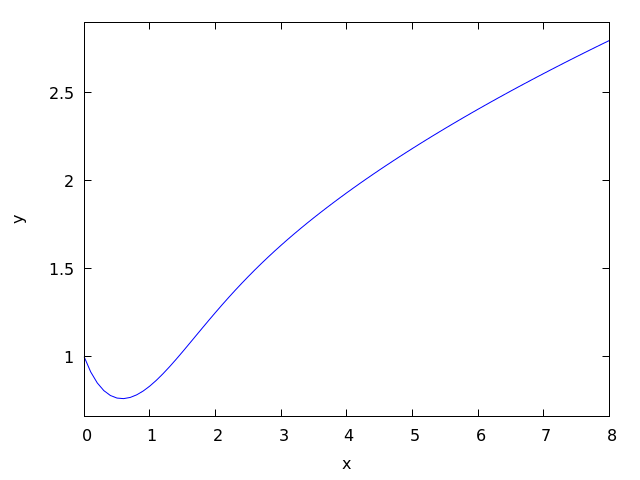
To solve numerically the differential equation

$${{dx}\over{dt}} = t - x^2$$

$${{dx}\over{dt}} = t - x^2$$

With initial value $x(t=0) = 1$, in the interval of $t$ from 0 to 8 and with increments of 0.1 for $t$, use:

maxima
(%i1) results: rk(t-x^2,x,1,[t,0,8,0.1])$
(%i2) plot2d ([discrete, results])$

The results will be saved in the list results and the plot will show the solution obtained, with t on the horizontal axis and x on the vertical axis.

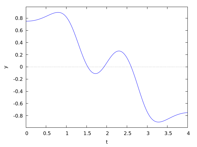
To solve numerically the system:

$$\eqalign{ {dx\over dy} &= 4-x^2-4y^2 \cr {dy\over dt} &= y^2 - x^2 + 1 }$$

$$\eqalign{ {dx\over dy} &= 4-x^2-4y^2 \cr {dy\over dt} &= y^2 - x^2 + 1 }$$

for $t$ between 0 and 4, and with values of -1.25 and 0.75 for $x$ and $y$ at $t=0$:

maxima

(%i1) sol: rk([4-x^2-4*y^2, y^2-x^2+1], [x, y], [-1.25, 0.75],
              [t,0,4,0.02])$


(%i2) plot2d([discrete, makelist([p[1], p[3]], p, sol)], [xlabel, "t"],
             [ylabel, "y"])$

The plot will show the solution for variable y as a function of t.

See also: drawdf, rk_adaptive, desolve, ode2.