Introduction
Reference documentation for Maxima’s built-in functions and variables, generated from the official Maxima Texinfo source.
Algebra
asympa
Function: asympa
asympa is a package for asymptotic analysis. The package contains
simplification functions for asymptotic analysis, including the “big O”
and “little o” functions that are widely used in complexity analysis and
numerical analysis.
load ("asympa") loads this package.
sym
comp2pui (n, L) — Function
implements passing from the complete symmetric functions given in the list L to the elementary symmetric functions from 0 to n. If the list L contains fewer than n+1 elements, it will be completed with formal values of the type h1, h2, etc. If the first element of the list L exists, it specifies the size of the alphabet, otherwise the size is set to n.
(%i1) comp2pui (3, [4, g]);
                        2                    2
(%o1)    [4, g, 2 h2 - g , 3 h3 - g h2 + g (g  - 2 h2)]
cont2part (pc, lvar) — Function
returns the partitioned polynomial associated to the contracted form pc whose variables are in lvar.
(%i1) pc: 2*a^3*b*x^4*y + x^5;
                           3    4      5
(%o1)                   2 a  b x  y + x


(%i2) cont2part (pc, [x, y]);
                                   3
(%o2)              [[1, 5, 0], [2 a  b, 4, 1]]
direct ([p_1, …, p_n], y, f, [lvar_1, …, lvar_n]) — Function
calculates the direct image (see M. Giusti, D. Lazard et A. Valibouze, ISSAC 1988, Rome) associated to the function f, in the lists of variables lvar_1, …, lvar_n, and in the polynomials p_1, …, p_n in a variable y. The arity of the function f is important for the calculation. Thus, if the expression for f does not depend on some variable, it is useless to include this variable, and not including it will also considerably reduce the amount of computation.
(%i1) direct ([z^2  - e1* z + e2, z^2  - f1* z + f2],
              z, b*v + a*u, [[u, v], [a, b]]);
       2
(%o1) y  - e1 f1 y

                                 2            2             2   2
                  - 4 e2 f2 - (e1  - 2 e2) (f1  - 2 f2) + e1  f1
                + -----------------------------------------------
                                         2


(%i2) ratsimp (%);
              2                2                   2
(%o2)        y  - e1 f1 y + (e1  - 4 e2) f2 + e2 f1


(%i3) ratsimp (direct ([z^3-e1*z^2+e2*z-e3,z^2  - f1* z + f2],
              z, b*v + a*u, [[u, v], [a, b]]));
       6            5         2                        2    2   4
(%o3) y  - 2 e1 f1 y  + ((2 e1  - 6 e2) f2 + (2 e2 + e1 ) f1 ) y

                          3                               3   3
 + ((9 e3 + 5 e1 e2 - 2 e1 ) f1 f2 + (- 2 e3 - 2 e1 e2) f1 ) y

         2       2        4    2
 + ((9 e2  - 6 e1  e2 + e1 ) f2

                    2       2       2                   2    4
 + (- 9 e1 e3 - 6 e2  + 3 e1  e2) f1  f2 + (2 e1 e3 + e2 ) f1 )

  2          2                      2     3          2
 y  + (((9 e1  - 27 e2) e3 + 3 e1 e2  - e1  e2) f1 f2

                 2            2    3                5
 + ((15 e2 - 2 e1 ) e3 - e1 e2 ) f1  f2 - 2 e2 e3 f1 ) y

           2                   3           3     2   2    3
 + (- 27 e3  + (18 e1 e2 - 4 e1 ) e3 - 4 e2  + e1  e2 ) f2

         2      3                   3    2   2
 + (27 e3  + (e1  - 9 e1 e2) e3 + e2 ) f1  f2

                   2    4        2   6
 + (e1 e2 e3 - 9 e3 ) f1  f2 + e3  f1
Finding the polynomial whose roots are the sums $a+u$ where $a$ is a root of $z^2 - e_1 z + e_2$ and $u$ is a root of $z^2 - f_1 z + f_2$.
(%i1) ratsimp (direct ([z^2 - e1* z + e2, z^2 - f1* z + f2],
                          z, a + u, [[u], [a]]));
       4                    3             2
(%o1) y  + (- 2 f1 - 2 e1) y  + (2 f2 + f1  + 3 e1 f1 + 2 e2

     2   2                              2               2
 + e1 ) y  + ((- 2 f1 - 2 e1) f2 - e1 f1  + (- 2 e2 - e1 ) f1

                  2                     2            2
 - 2 e1 e2) y + f2  + (e1 f1 - 2 e2 + e1 ) f2 + e2 f1  + e1 e2 f1

     2
 + e2
direct accepts two flags: elementaires and
puissances (default) which allow decomposing the symmetric
polynomials appearing in the calculation into elementary symmetric
functions, or power functions, respectively.
Functions of sym used in this function:
multi_orbit (so orbit), pui_direct, multi_elem
(so elem), multi_pui (so pui), pui2ele, ele2pui
(if the flag direct is in puissances).
ele2comp (m, L) — Function
Goes from the elementary symmetric functions to the compete functions.
Similar to comp2ele and comp2pui.
Other functions for changing bases: comp2ele.
ele2polynome (L, z) — Function
returns the polynomial in z s.t. the elementary symmetric
functions of its roots are in the list L = [n, e_1, ..., e_n], where n is the degree of the
polynomial and e_i the i-th elementary symmetric function.
(%i1) ele2polynome ([2, e1, e2], z);
                          2
(%o1)                    z  - e1 z + e2


(%i2) polynome2ele (x^7 - 14*x^5 + 56*x^3  - 56*x + 22, x);
(%o2)          [7, 0, - 14, 0, 56, 0, - 56, - 22]


(%i3) ele2polynome ([7, 0, -14, 0, 56, 0, -56, -22], x);
                  7       5       3
(%o3)            x  - 14 x  + 56 x  - 56 x + 22
The inverse: polynome2ele (P, z).
Also see:
polynome2ele, pui2polynome.
ele2pui (m, L) — Function
goes from the elementary symmetric functions to the complete functions.
Similar to comp2ele and comp2pui.
Other functions for changing bases: comp2ele.
elem (ele, sym, lvar) — Function
decomposes the symmetric polynomial sym, in the variables
contained in the list lvar, in terms of the elementary symmetric
functions given in the list ele. If the first element of
ele is given, it will be the size of the alphabet, otherwise the
size will be the degree of the polynomial sym. If values are
missing in the list ele, formal values of the type e1,
e2, etc. will be added. The polynomial sym may be given in
three different forms: contracted (elem should then be 1, its
default value), partitioned (elem should be 3), or extended
(i.e. the entire polynomial, and elem should then be 2). The
function pui is used in the same way.
On an alphabet of size 3 with e1, the first elementary symmetric function, with value 7, the symmetric polynomial in 3 variables whose contracted form (which here depends on only two of its variables) is x^4-2xy decomposes as follows in elementary symmetric functions:
(%i1) elem ([3, 7], x^4 - 2*x*y, [x, y]);
(%o1) 7 (e3 - 7 e2 + 7 (49 - e2)) + 21 e3

                                         + (- 2 (49 - e2) - 2) e2


(%i2) ratsimp (%);
                              2
(%o2)             28 e3 + 2 e2  - 198 e2 + 2401
Other functions for changing bases: comp2ele.
explose (pc, lvar) — Function
returns the symmetric polynomial associated with the contracted form pc. The list lvar contains the variables.
(%i1) explose (a*x + 1, [x, y, z]);
(%o1)                  a z + a y + a x + 1
kostka (part_1, part_2) — Function
written by P. Esperet, calculates the Kostka number of the partition part_1 and part_2.
(%i1) kostka ([3, 3, 3], [2, 2, 2, 1, 1, 1]);
(%o1)                           6
lgtreillis (n, m) — Function
returns the list of partitions of weight n and length m.
(%i1) lgtreillis (4, 2);
(%o1)                   [[3, 1], [2, 2]]
Also see: ltreillis, treillis and treinat.
See also: ltreillis, treillis, treinat.
ltreillis (n, m) — Function
returns the list of partitions of weight n and length less than or equal to m.
(%i1) ltreillis (4, 2);
(%o1)               [[4, 0], [3, 1], [2, 2]]
Also see: lgtreillis, treillis and treinat.
See also: lgtreillis, treillis, treinat.
mon2schur (L) — Function
The list L represents the Schur function $S_L$: we have $L = [i_1, i_2, …, i_q]$, with $i_1 <= i_2 <= … <= i_q$. The Schur function $S_[i_1, i_2, …, i_q]$ is the minor of the infinite matrix $h_[i-j]$, $i <= 1, j <= 1$, consisting of the $q$ first rows and the columns $1 + i_1, 2 + i_2, …, q + i_q$.
This Schur function can be written in terms of monomials by using
treinat and kostka. The form returned is a symmetric
polynomial in a contracted representation in the variables
$x_1,x_2,\ldots$
$x_1,x_2,…$
(%i1) mon2schur ([1, 1, 1]);
(%o1)                       x1 x2 x3


(%i2) mon2schur ([3]);
                                  2        3
(%o2)                x1 x2 x3 + x1  x2 + x1


(%i3) mon2schur ([1, 2]);
                                      2
(%o3)                  2 x1 x2 x3 + x1  x2
which means that for 3 variables this gives:
2 x1 x2 x3 + x1^2 x2 + x2^2 x1 + x1^2 x3 + x3^2 x1
    + x2^2 x3 + x3^2 x2
Other functions for changing bases: comp2ele.
See also: treinat, kostka.
multi_elem (l_elem, multi_pc, l_var) — Function
decomposes a multi-symmetric polynomial in the multi-contracted form multi_pc in the groups of variables contained in the list of lists l_var in terms of the elementary symmetric functions contained in l_elem.
(%i1) multi_elem ([[2, e1, e2], [2, f1, f2]], a*x + a^2 + x^3,
      [[x, y], [a, b]]);
                                                  3
(%o1)         - 2 f2 + f1 (f1 + e1) - 3 e1 e2 + e1


(%i2) ratsimp (%);
                         2                       3
(%o2)         - 2 f2 + f1  + e1 f1 - 3 e1 e2 + e1
Other functions for changing bases: comp2ele.
multi_orbit (P, [lvar_1, lvar_2, …, lvar_p]) — Function
P is a polynomial in the set of variables contained in the lists lvar_1, lvar_2, …, lvar_p. This function returns the orbit of the polynomial P under the action of the product of the symmetric groups of the sets of variables represented in these p lists.
(%i1) multi_orbit (a*x + b*y, [[x, y], [a, b]]);
(%o1)                [b y + a x, a y + b x]


(%i2) multi_orbit (x + y + 2*a, [[x, y], [a, b, c]]);
(%o2)        [y + x + 2 c, y + x + 2 b, y + x + 2 a]
Also see: orbit for the action of a single symmetric group.
Function: multi_pui
is to the function pui what the function multi_elem is to
the function elem.
(%i1) multi_pui ([[2, p1, p2], [2, t1, t2]], a*x + a^2 + x^3,
      [[x, y], [a, b]]);
                                            3
                                3 p1 p2   p1
(%o1)              t2 + p1 t1 + ------- - ---
                                   2       2
multinomial (r, part) — Function
where r is the weight of the partition part. This function
returns the associate multinomial coefficient: if the parts of
part are i_1, i_2, …, i_k, the result is
r!/(i_1! i_2! ... i_k!).
multsym (ppart_1, ppart_2, n) — Function
returns the product of the two symmetric polynomials in n variables by working only modulo the action of the symmetric group of order n. The polynomials are in their partitioned form.
Given the 2 symmetric polynomials in x, y: 3*(x + y) + 2*x*y and 5*(x^2 + y^2) whose partitioned forms are [[3, 1], [2, 1, 1]] and [[5, 2]], their product will be
(%i1) multsym ([[3, 1], [2, 1, 1]], [[5, 2]], 2);
(%o1)         [[10, 3, 1], [15, 3, 0], [15, 2, 1]]
that is 10*(x^3*y + y^3*x) + 15*(x^2*y + y^2*x) + 15*(x^3 + y^3).
Functions for changing the representations of a symmetric polynomial:
contract, cont2part, explose, part2cont,
partpol, tcontract, tpartpol.
orbit (P, lvar) — Function
computes the orbit of the polynomial P in the variables in the list lvar under the action of the symmetric group of the set of variables in the list lvar.
(%i1) orbit (a*x + b*y, [x, y]);
(%o1)                [a y + b x, b y + a x]


(%i2) orbit (2*x + x^2, [x, y]);
                        2         2
(%o2)                 [y  + 2 y, x  + 2 x]
See also multi_orbit for the action of a product of symmetric
groups on a polynomial.
See also: multi_orbit.
part2cont (ppart, lvar) — Function
goes from the partitioned form to the contracted form of a symmetric polynomial. The contracted form is rendered with the variables in lvar.
(%i1) part2cont ([[2*a^3*b, 4, 1]], [x, y]);
                              3    4
(%o1)                      2 a  b x  y
partpol (psym, lvar) — Function
psym is a symmetric polynomial in the variables of the list lvar. This function returns its partitioned representation.
(%i1) partpol (-a*(x + y) + 3*x*y, [x, y]);
(%o1)               [[3, 1, 1], [- a, 1, 0]]
permut (L) — Function
returns the list of permutations of the list L.
polynome2ele (P, x) — Function
gives the list l = [n, e_1, ..., e_n]
where n is the degree of the polynomial P in the variable
x and e_i is the i-the elementary symmetric function
of the roots of P.
(%i1) polynome2ele (x^7 - 14*x^5 + 56*x^3 - 56*x + 22, x);
(%o1)          [7, 0, - 14, 0, 56, 0, - 56, - 22]


(%i2) ele2polynome ([7, 0, -14, 0, 56, 0, -56, -22], x);
                  7       5       3
(%o2)            x  - 14 x  + 56 x  - 56 x + 22
The inverse: ele2polynome (l, x)
prodrac (L, k) — Function
L is a list containing the elementary symmetric functions
on a set A. prodrac returns the polynomial whose roots
are the k by k products of the elements of A.
Also see somrac.
pui (L, sym, lvar) — Function
decomposes the symmetric polynomial sym, in the variables in the
list lvar, in terms of the power functions in the list L.
If the first element of L is given, it will be the size of the
alphabet, otherwise the size will be the degree of the polynomial
sym. If values are missing in the list L, formal values of
the type p1, p2 , etc. will be added. The polynomial
sym may be given in three different forms: contracted (elem
should then be 1, its default value), partitioned (elem should be
3), or extended (i.e. the entire polynomial, and elem should then
be 2). The function pui is used in the same way.
(%i1) pui;
(%o1)                           1


(%i2) pui ([3, a, b], u*x*y*z, [x, y, z]);
                       2
                   a (a  - b) u   (a b - p3) u
(%o2)              ------------ - ------------
                        6              3


(%i3) ratsimp (%);
                                       3
                      (2 p3 - 3 a b + a ) u
(%o3)                 ---------------------
                                6
Other functions for changing bases: comp2ele.
pui2comp (n, lpui) — Function
renders the list of the first n complete functions (with the
length first) in terms of the power functions given in the list
lpui. If the list lpui is empty, the cardinal is n,
otherwise it is its first element (as in comp2ele and
comp2pui).
(%i1) pui2comp (2, []);
                                       2
                                p2 + p1
(%o1)                   [2, p1, --------]
                                   2


(%i2) pui2comp (3, [2, a1]);
                                            2
                                 a1 (p2 + a1 )
                         2  p3 + ------------- + a1 p2
                  p2 + a1              2
(%o2)     [2, a1, --------, --------------------------]
                     2                  3


(%i3) ratsimp (%);
                            2                     3
                     p2 + a1   2 p3 + 3 a1 p2 + a1
(%o3)        [2, a1, --------, --------------------]
                        2               6
Other functions for changing bases: comp2ele.
pui2ele (n, lpui) — Function
effects the passage from power functions to the elementary symmetric functions.
If the flag pui2ele is girard, it will return the list of
elementary symmetric functions from 1 to n, and if the flag is
close, it will return the n-th elementary symmetric function.
Other functions for changing bases: comp2ele.
pui2polynome (x, lpui) — Function
calculates the polynomial in x whose power functions of the roots are given in the list lpui.
(%i1) pui;
(%o1)                           1


(%i2) kill(labels);
(%o0)                         done


(%i1) polynome2ele (x^3 - 4*x^2 + 5*x - 1, x);
(%o1)                     [3, 4, 5, 1]


(%i2) ele2pui (3, %);
(%o2)                     [3, 4, 6, 7]


(%i3) pui2polynome (x, %);
                        3      2
(%o3)                  x  - 4 x  + 5 x - 1
See also:
polynome2ele, ele2polynome.
See also: polynome2ele, ele2polynome.
pui_direct (orbite, [lvar_1, …, lvar_n], [d_1, d_2, …, d_n]) — Function
Let f be a polynomial in n blocks of variables lvar_1,
…, lvar_n. Let c_i be the number of variables in
lvar_i, and SC be the product of n symmetric groups of
degree c_1, …, c_n. This group acts naturally on f.
The list orbite is the orbit, denoted SC(f), of
the function f under the action of SC. (This list may be
obtained by the function multi_orbit.) The di are integers
s.t.
$c_1 <= d_1, c_2 <= d_2, …, c_n <= d_n$.
Let SD be the product of the symmetric groups $S_[d_1] x S_[d_2] x … x S_[d_n]$.
The function pui_direct returns
the first n power functions of SD(f) deduced
from the power functions of SC(f), where n is
the size of SD(f).
The result is in multi-contracted form w.r.t. SD, i.e. only one element is kept per orbit, under the action of SD.
(%i1) l: [[x, y], [a, b]];
(%o1)                   [[x, y], [a, b]]


(%i2) pui_direct (multi_orbit (a*x + b*y, l), l, [2, 2]);
                                       2  2
(%o2)               [a x, 4 a b x y + a  x ]


(%i3) pui_direct (multi_orbit (a*x + b*y, l), l, [3, 2]);
                             2  2     2    2        3  3
(%o3) [2 a x, 4 a b x y + 2 a  x , 3 a  b x  y + 2 a  x ,

    2  2  2  2      3    3        4  4
12 a  b  x  y  + 4 a  b x  y + 2 a  x ,

    3  2  3  2      4    4        5  5
10 a  b  x  y  + 5 a  b x  y + 2 a  x ,

    3  3  3  3       4  2  4  2      5    5        6  6
40 a  b  x  y  + 15 a  b  x  y  + 6 a  b x  y + 2 a  x ]


(%i4) pui_direct ([y + x + 2*c, y + x + 2*b, y + x + 2*a],
      [[x, y], [a, b, c]], [2, 3]);
                             2              2
(%o4) [3 x + 2 a, 6 x y + 3 x  + 4 a x + 4 a ,

                 2                   3        2       2        3
              9 x  y + 12 a x y + 3 x  + 6 a x  + 12 a  x + 8 a ]
puireduc (n, lpui) — Function
lpui is a list whose first element is an integer m.
puireduc gives the first n power functions in terms of the
first m.
(%i1) puireduc (3, [2]);
                                         2
                                   p1 (p1  - p2)
(%o1)          [2, p1, p2, p1 p2 - -------------]
                                         2


(%i2) ratsimp (%);
                                           3
                               3 p1 p2 - p1
(%o2)              [2, p1, p2, -------------]
                                     2
resolvante (P, x, f, [x_1, …, x_d]) — Function
calculates the resolvent of the polynomial P in x of degree
n >= d by the function f expressed in the variables
x_1, …, x_d. For efficiency of computation it is
important to not include in the list [x_1, ..., x_d]
variables which do not appear in the transformation function f.
To increase the efficiency of the computation one may set flags in
resolvante so as to use appropriate algorithms:
If the function f is unitary:
A polynomial in a single variable,
linear,
alternating,
a sum,
symmetric,
a product,
the function of the Cayley resolvent (usable up to degree 5)
(x1*x2 + x2*x3 + x3*x4 + x4*x5 + x5*x1 -
     (x1*x3 + x3*x5 + x5*x2 + x2*x4 + x4*x1))^2
general,
the flag of resolvante may be, respectively:
unitaire,
lineaire,
alternee,
somme,
produit,
cayley,
generale.
(%i1) resolvante: unitaire$

(%i2) resolvante (x^7 - 14*x^5 + 56*x^3 - 56*x + 22, x, x^3 - 1,
      [x]);

" resolvante unitaire " [7, 0, 28, 0, 168, 0, 1120, - 154, 7840,
                         - 2772, 56448, - 33880,

413952, - 352352, 3076668, - 3363360, 23114112, - 30494464,

175230832, - 267412992, 1338886528, - 2292126760]
  3       6      3       9      6      3
[x  - 1, x  - 2 x  + 1, x  - 3 x  + 3 x  - 1,

 12      9      6      3       15      12       9       6      3
x   - 4 x  + 6 x  - 4 x  + 1, x   - 5 x   + 10 x  - 10 x  + 5 x

       18      15       12       9       6      3
 - 1, x   - 6 x   + 15 x   - 20 x  + 15 x  - 6 x  + 1,

 21      18       15       12       9       6      3
x   - 7 x   + 21 x   - 35 x   + 35 x  - 21 x  + 7 x  - 1]
[- 7, 1127, - 6139, 431767, - 5472047, 201692519, - 3603982011]
       7      6        5         4          3           2
(%o2) y  + 7 y  - 539 y  - 1841 y  + 51443 y  + 315133 y

                                              + 376999 y + 125253

(%i3) resolvante: lineaire$

(%i4) resolvante (x^4 - 1, x, x1 + 2*x2 + 3*x3, [x1, x2, x3]);

" resolvante lineaire "
       24       20         16            12             8
(%o4) y   + 80 y   + 7520 y   + 1107200 y   + 49475840 y

                                                    4
                                       + 344489984 y  + 655360000

(%i5) resolvante: general$

(%i6) resolvante (x^4 - 1, x, x1 + 2*x2 + 3*x3, [x1, x2, x3]);

" resolvante generale "
       24       20         16            12             8
(%o6) y   + 80 y   + 7520 y   + 1107200 y   + 49475840 y

                                                    4
                                       + 344489984 y  + 655360000


(%i7) resolvante (x^4 - 1, x, x1 + 2*x2 + 3*x3, [x1, x2, x3, x4]);

" resolvante generale "
       24       20         16            12             8
(%o7) y   + 80 y   + 7520 y   + 1107200 y   + 49475840 y

                                                    4
                                       + 344489984 y  + 655360000


(%i8) direct ([x^4 - 1], x, x1 + 2*x2 + 3*x3, [[x1, x2, x3]]);
       24       20         16            12             8
(%o8) y   + 80 y   + 7520 y   + 1107200 y   + 49475840 y

                                                    4
                                       + 344489984 y  + 655360000

(%i9) resolvante :lineaire$

(%i10) resolvante (x^4 - 1, x, x1 + x2 + x3, [x1, x2, x3]);

" resolvante lineaire "
                              4
(%o10)                       y  - 1

(%i11) resolvante: symetrique$

(%i12) resolvante (x^4 - 1, x, x1 + x2 + x3, [x1, x2, x3]);

" resolvante symetrique "
                              4
(%o12)                       y  - 1


(%i13) resolvante (x^4 + x + 1, x, x1 - x2, [x1, x2]);

" resolvante symetrique "
                           6      2
(%o13)                    y  - 4 y  - 1

(%i14) resolvante: alternee$

(%i15) resolvante (x^4 + x + 1, x, x1 - x2, [x1, x2]);

" resolvante alternee "
            12      8       6        4        2
(%o15)     y   + 8 y  + 26 y  - 112 y  + 216 y  + 229

(%i16) resolvante: produit$

(%i17) resolvante (x^7 - 7*x + 3, x, x1*x2*x3, [x1, x2, x3]);

" resolvante produit "
        35      33         29        28         27        26
(%o17) y   - 7 y   - 1029 y   + 135 y   + 7203 y   - 756 y

         24           23          22            21           20
 + 1323 y   + 352947 y   - 46305 y   - 2463339 y   + 324135 y

          19           18             17              15
 - 30618 y   - 453789 y   - 40246444 y   + 282225202 y

             14              12             11            10
 - 44274492 y   + 155098503 y   + 12252303 y   + 2893401 y

              9            8            7             6
 - 171532242 y  + 6751269 y  + 2657205 y  - 94517766 y

            5             3
 - 3720087 y  + 26040609 y  + 14348907

(%i18) resolvante: symetrique$

(%i19) resolvante (x^7 - 7*x + 3, x, x1*x2*x3, [x1, x2, x3]);

" resolvante symetrique "
        35      33         29        28         27        26
(%o19) y   - 7 y   - 1029 y   + 135 y   + 7203 y   - 756 y

         24           23          22            21           20
 + 1323 y   + 352947 y   - 46305 y   - 2463339 y   + 324135 y

          19           18             17              15
 - 30618 y   - 453789 y   - 40246444 y   + 282225202 y

             14              12             11            10
 - 44274492 y   + 155098503 y   + 12252303 y   + 2893401 y

              9            8            7             6
 - 171532242 y  + 6751269 y  + 2657205 y  - 94517766 y

            5             3
 - 3720087 y  + 26040609 y  + 14348907

(%i20) resolvante: cayley$

(%i21) resolvante (x^5 - 4*x^2 + x + 1, x, a, []);

" resolvante de Cayley "
        6       5         4          3            2
(%o21) x  - 40 x  + 4080 x  - 92928 x  + 3772160 x  + 37880832 x

                                                       + 93392896
For the Cayley resolvent, the 2 last arguments are neutral and the input polynomial must necessarily be of degree 5.
See also:
resolvante_bipartite, resolvante_produit_sym,
resolvante_unitaire, resolvante_alternee1, resolvante_klein,
resolvante_klein3, resolvante_vierer, resolvante_005fdiedrale.
See also: resolvante_bipartite, resolvante_produit_sym, resolvante_unitaire, resolvante_alternee1, resolvante_klein, resolvante_klein3, resolvante_vierer, resolvante_diedrale.
resolvante_alternee1 (P, x) — Function
calculates the transformation
P(x) of degree n by the function
$product(x_i - x_j, 1 <= i < j <= n - 1)$.
See also:
resolvante_produit_sym, resolvante_unitaire,
resolvante, resolvante_klein, resolvante_klein3,
resolvante_vierer, resolvante_diedrale, resolvante_005fbipartite.
See also: resolvante_produit_sym, resolvante_unitaire, resolvante, resolvante_klein, resolvante_klein3, resolvante_vierer, resolvante_diedrale, resolvante_bipartite.
resolvante_bipartite (P, x) — Function
calculates the transformation of
P(x) of even degree n by the function
$x_1 x_2 … x_[n/2] + x_[n/2 + 1] … x_n$.
(%i1) resolvante_bipartite (x^6 + 108, x);
              10        8           6             4
(%o1)        y   - 972 y  + 314928 y  - 34012224 y
See also:
resolvante_produit_sym, resolvante_unitaire,
resolvante, resolvante_klein, resolvante_klein3,
resolvante_vierer, resolvante_diedrale, resolvante_005falternee1.
See also: resolvante_produit_sym, resolvante_unitaire, resolvante, resolvante_klein, resolvante_klein3, resolvante_vierer, resolvante_diedrale, resolvante_alternee1.
resolvante_diedrale (P, x) — Function
calculates the transformation of P(x) by the function
x_1 x_2 + x_3 x_4.
(%i1) resolvante_diedrale (x^5 - 3*x^4 + 1, x);
       15       12       11       10        9         8         7
(%o1) x   - 21 x   - 81 x   - 21 x   + 207 x  + 1134 x  + 2331 x

        6         5          4          3          2
 - 945 x  - 4970 x  - 18333 x  - 29079 x  - 20745 x  - 25326 x

 - 697
See also:
resolvante_produit_sym, resolvante_unitaire,
resolvante_alternee1, resolvante_klein, resolvante_klein3,
resolvante_vierer, resolvante.
See also: resolvante_produit_sym, resolvante_unitaire, resolvante_alternee1, resolvante_klein, resolvante_klein3, resolvante_vierer, resolvante.
resolvante_klein (P, x) — Function
calculates the transformation of P(x) by the function
x_1 x_2 x_4 + x_4.
See also:
resolvante_produit_sym, resolvante_unitaire,
resolvante_alternee1, resolvante, resolvante_klein3,
resolvante_vierer, resolvante_005fdiedrale.
See also: resolvante_produit_sym, resolvante_unitaire, resolvante_alternee1, resolvante, resolvante_klein3, resolvante_vierer, resolvante_diedrale.
resolvante_klein3 (P, x) — Function
calculates the transformation of P(x) by the function
x_1 x_2 x_4 + x_4.
See also:
resolvante_produit_sym, resolvante_unitaire,
resolvante_alternee1, resolvante_klein, resolvante,
resolvante_vierer, resolvante_005fdiedrale.
See also: resolvante_produit_sym, resolvante_unitaire, resolvante_alternee1, resolvante_klein, resolvante, resolvante_vierer, resolvante_diedrale.
resolvante_produit_sym (P, x) — Function
calculates the list of all product resolvents of the polynomial
P(x).
(%i1) resolvante_produit_sym (x^5 + 3*x^4 + 2*x - 1, x);
        5      4             10      8       7       6       5
(%o1) [y  + 3 y  + 2 y - 1, y   - 2 y  - 21 y  - 31 y  - 14 y

    4       3      2       10      8       7    6       5       4
 - y  + 14 y  + 3 y  + 1, y   + 3 y  + 14 y  - y  - 14 y  - 31 y

       3      2       5      4
 - 21 y  - 2 y  + 1, y  - 2 y  - 3 y - 1, y - 1]

(%i2) resolvante: produit$

(%i3) resolvante (x^5 + 3*x^4 + 2*x - 1, x, a*b*c, [a, b, c]);

" resolvante produit "
       10      8       7    6        5       4       3     2
(%o3) y   + 3 y  + 14 y  - y  - 14 y  - 31 y  - 21 y  - 2 y  + 1
See also:
resolvante, resolvante_unitaire,
resolvante_alternee1, resolvante_klein,
resolvante_klein3, resolvante_vierer,
resolvante_005fdiedrale.
See also: resolvante, resolvante_unitaire, resolvante_alternee1, resolvante_klein, resolvante_klein3, resolvante_vierer, resolvante_diedrale.
resolvante_unitaire (P, Q, x) — Function
computes the resolvent of the polynomial P(x) by the
polynomial Q(x).
See also:
resolvante_produit_sym, resolvante,
resolvante_alternee1, resolvante_klein, resolvante_klein3,
resolvante_vierer, resolvante_005fdiedrale.
See also: resolvante_produit_sym, resolvante, resolvante_alternee1, resolvante_klein, resolvante_klein3, resolvante_vierer, resolvante_diedrale.
resolvante_vierer (P, x) — Function
computes the transformation of
P(x) by the function x_1 x_2 - x_3 x_4.
See also:
resolvante_produit_sym, resolvante_unitaire,
resolvante_alternee1, resolvante_klein, resolvante_klein3,
resolvante, resolvante_005fdiedrale.
See also: resolvante_produit_sym, resolvante_unitaire, resolvante_alternee1, resolvante_klein, resolvante_klein3, resolvante, resolvante_diedrale.
schur2comp (P, l_var) — Function
P is a polynomial in the variables of the list l_var. Each
of these variables represents a complete symmetric function. In
l_var the i-th complete symmetric function is represented by
the concatenation of the letter h and the integer i:
hi. This function expresses P in terms of Schur
functions.
(%i1) schur2comp (h1*h2 - h3, [h1, h2, h3]);
(%o1)                         s
                               1, 2


(%i2) schur2comp (a*h3, [h3]);
(%o2)                         s  a
                               3
somrac (L, k) — Function
The list L contains elementary symmetric functions of a polynomial P . The function computes the polynomial whose roots are the k by k distinct sums of the roots of P.
Also see prodrac.
tcontract (pol, lvar) — Function
tests if the polynomial pol is symmetric in the variables of the
list lvar. If so, it returns a contracted representation like the
function contract.
tpartpol (pol, lvar) — Function
tests if the polynomial pol is symmetric in the variables of the
list lvar. If so, it returns its partitioned representation like
the function partpol.
treillis (n) — Function
returns all partitions of weight n.
(%i1) treillis (4);
(%o1)    [[4], [3, 1], [2, 2], [2, 1, 1], [1, 1, 1, 1]]
See also: lgtreillis, ltreillis and treinat.
See also: lgtreillis, ltreillis, treinat.
treinat (part) — Function
returns the list of partitions inferior to the partition part w.r.t. the natural order.
(%i1) treinat ([5]);
(%o1)                         [[5]]


(%i2) treinat ([1, 1, 1, 1, 1]);
(%o2) [[5], [4, 1], [3, 2], [3, 1, 1], [2, 2, 1], [2, 1, 1, 1],

                                                 [1, 1, 1, 1, 1]]


(%i3) treinat ([3, 2]);
(%o3)                 [[5], [4, 1], [3, 2]]
See also: lgtreillis, ltreillis and treillis.
See also: lgtreillis, ltreillis, treillis.
Calculus
Differential Equations
%c — Variable
%c is the integration constant in the solutions of first
order ODEs returned from ode2.
See also: ode2.
%k1 — Variable
%k1 is the first integration constant in the solutions of second
order ODEs returned from ode2.
See also: ode2.
%k2 — Variable
%k2 is the second integration constant in the solutions of second
order ODEs returned from ode2.
See also: ode2.
bc2 (solution, xval1, yval1, xval2, yval2) — Function
Solves a boundary value problem for a second order differential equation.
Here: solution is a general solution to the equation, as found by
ode2; xval1 specifies the value of the independent variable
in a first point, in the form x = x1, and yval1
gives the value of the dependent variable in that point, in the form
y = y1. The expressions xval2 and yval2
give the values for these variables at a second point, using the same
form.
See ode2 for an example of its usage.
See also: ode2.
desolve (eqn, y) — Function
The function desolve solves systems of linear ordinary
differential equations using Laplace transform. Here the eqn’s are
differential equations in the dependent variables y_1, …,
y_n. The functional dependence of y_1, …, y_n on an
independent variable, for instance x, must be explicitly indicated
in the variables and its derivatives. For example, the correct
way to define the differential equations would be:
eqn_1: 'diff(f(x),x,2) = sin(x) + 'diff(g(x),x);
eqn_2: 'diff(f(x),x) + x^2 - f(x) = 2*'diff(g(x),x,2);
The call to the function desolve would then be:
desolve([eqn_1, eqn_2], [f(x),g(x)]);
If initial conditions at x=0 are known, they can be supplied before
calling desolve by using atvalue.
maxima

(%i1) 'diff(f(x),x)='diff(g(x),x)+sin(x);
                 d           d
(%o1)            -- (f(x)) = -- (g(x)) + sin(x)
                 dx          dx


(%i2) 'diff(g(x),x,2)='diff(f(x),x)-cos(x);
                  2
                 d            d
(%o2)            --- (g(x)) = -- (f(x)) - cos(x)
                   2          dx
                 dx


(%i3) atvalue('diff(g(x),x),x=0,a);
(%o3)                           a


(%i4) atvalue(f(x),x=0,1);
(%o4)                           1


(%i5) desolve([%o1,%o2],[f(x),g(x)]);
                x
(%o5) [f(x) = %e  a - a + 1, g(x) =
                                              x
                                   cos(x) + %e  a - a + g(0) - 1]


(%i6) [%o1,%o2],%o5,diff;
           x       x      x                x
(%o6)   [%e  a = %e  a, %e  a - cos(x) = %e  a - cos(x)]
If desolve cannot obtain a solution, it returns false.
See also ode2, drawdf and rk.
See also: atvalue, ode2, drawdf, rk.
ic1 (solution, xval, yval) — Function
Solves initial value problems for first order differential equations.
Here solution is a general solution to the equation, as found by
ode2, xval gives an initial value for the independent
variable in the form x = x0, and yval gives the
initial value for the dependent variable in the form y = y0.
See ode2 for an example of its usage.
See also: ode2.
ic2 (solution, xval, yval, dval) — Function
Solves initial value problems for second-order differential equations.
Here solution is a general solution to the equation, as found by
ode2, xval gives the initial value for the independent
variable in the form x = x0, yval gives the
initial value of the dependent variable in the form y = y0, and dval gives the initial value for the first
derivative of the dependent variable with respect to independent
variable, in the form 'diff(y,x) = dy0.
See ode2 for an example of its usage.
See also: ode2.
method — Variable
The variable method is set by ode2 to the successful solution
method.
See also: ode2.
ode2 (eqn, dvar, ivar) — Function
The function ode2 solves an ordinary differential equation (ODE)
of first or second order. It takes three arguments: an ODE given by
eqn, the dependent variable dvar, and the independent
variable ivar. When successful, it returns either an explicit or
implicit solution for the dependent variable. %c is used to
represent the integration constant in the case of first-order equations,
and %k1 and %k2 the constants for second-order
equations. The dependence of the dependent variable on the independent
variable does not have to be written explicitly, as in the case of
desolve, but the independent variable must always be given as the
third argument.
If ode2 cannot obtain a solution for whatever reason, it returns
false, after perhaps printing out an error message. The methods
implemented for first order equations in the order in which they are
tested are: linear, separable, exact - perhaps requiring an integrating
factor, homogeneous, Bernoulli’s equation, and a generalized homogeneous
method. The types of second-order equations which can be solved are:
constant coefficients, exact, linear homogeneous with non-constant
coefficients which can be transformed to constant coefficients, the
Euler or equi-dimensional equation, equations solvable by the method of
variation of parameters, and equations which are free of either the
independent or of the dependent variable so that they can be reduced to
two first order linear equations to be solved sequentially.
In the course of solving ODE’s, several variables are set purely for
informational purposes: method denotes the method of solution
used (e.g., linear), intfactor denotes any integrating
factor used, odeindex denotes the index for Bernoulli’s method or
for the generalized homogeneous method, and yp denotes the
particular solution for the variation of parameters technique.
In order to solve initial value problems (IVP) functions ic1 and
ic2 are available for first and second order equations, and to
solve second-order boundary value problems (BVP) the function bc2
can be used.
See also desolve, drawdf and rk.
Example:
maxima

(%i1) x^2*'diff(y,x) + 3*y*x = sin(x)/x;
                      2 dy           sin(x)
(%o1)                x  -- + 3 x y = ------
                        dx             x


(%i2) soln1: ode2(%,y,x);
                             %c - cos(x)
(%o2)                    y = -----------
                                  3
                                 x


(%i3) ic1 (soln1,x=%pi,y=0);
                              cos(x) + 1
(%o3)                   y = - ----------
                                   3
                                  x


(%i4) 'diff(y,x,2) + y*'diff(y,x)^3 = 0;
                         2
                        d y      dy 3
(%o4)                   --- + y (--)  = 0
                          2      dx
                        dx


(%i5) soln2: ode2(%,y,x);
                      3
                     y  + 6 %k1 y
(%o5)                ------------ = x + %k2
                          6


(%i6) ratsimp (ic2(soln2,x=0,y=0,'diff(y,x)=2));
                           3
                          y  + 3 y
(%o6)                     -------- = x
                             6


(%i7) bc2 (soln2,x=0,y=1,x=1,y=3);
                         3
                        y  - 10 y       3
(%o7)                   --------- = x - -
                            6           2
See also: %c, %k1, %k2, desolve, method, yp, ic1, ic2, bc2, drawdf, rk.
yp — Variable
yp is the particular solution of an ODE found by ode2
when using the variation of parameters technique.
See also: yp, ode2.
Differentiation
antid (expr, x, u(x)) — Function
Returns a two-element list, such that an antiderivative of expr with respect to x can be constructed from the list. The expression expr may contain an unknown function u and its derivatives.
Let L, a list of two elements, be the return value of antid.
Then L[1] + 'integrate (L[2], x)
is an antiderivative of expr with respect to x.
When antid succeeds entirely,
the second element of the return value is zero.
Otherwise, the second element is nonzero,
and the first element is nonzero or zero.
If antid cannot make any progress,
the first element is zero and the second nonzero.
load ("antid") loads this function. The antid package also
defines the functions nonzeroandfreeof and linear.
antid is related to antidiff as follows.
Let L, a list of two elements, be the return value of antid.
Then the return value of antidiff is equal to
L[1] + 'integrate (L[2], x) where x is the
variable of integration.
Examples:
maxima
(%i1) load ("antid")$

(%i2) expr: exp (z(x)) * diff (z(x), x) * y(x);
                       z(x)       d
(%o2)                %e     y(x) (-- (z(x)))
                                  dx


(%i3) a1: antid (expr, x, z(x));
                  z(x)           z(x)  d
(%o3)          [%e     y(x), - %e     (-- (y(x)))]
                                       dx


(%i4) a2: antidiff (expr, x, z(x));
                            /
                z(x)        |   z(x)  d
(%o4)         %e     y(x) - | %e     (-- (y(x))) dx
                            |         dx
                            /


(%i5) a2 - (first (a1) + 'integrate (second (a1), x));
(%o5)                           0


(%i6) antid (expr, x, y(x));
                        z(x)       d
(%o6)             [0, %e     y(x) (-- (z(x)))]
                                   dx


(%i7) antidiff (expr, x, y(x));
                  /
                  |   z(x)       d
(%o7)             | %e     y(x) (-- (z(x))) dx
                  |              dx
                  /
See also: antidiff.
antidiff (expr, x, u(x)) — Function
Returns an antiderivative of expr with respect to x. The expression expr may contain an unknown function u and its derivatives.
When antidiff succeeds entirely, the resulting expression is free of
integral signs (that is, free of the integrate noun).
Otherwise, antidiff returns an expression
which is partly or entirely within an integral sign.
If antidiff cannot make any progress,
the return value is entirely within an integral sign.
load ("antid") loads this function.
The antid package also defines the functions nonzeroandfreeof and
linear.
antidiff is related to antid as follows.
Let L, a list of two elements, be the return value of antid.
Then the return value of antidiff is equal to
L[1] + 'integrate (L[2], x) where x is the
variable of integration.
Examples:
maxima
(%i1) load ("antid")$

(%i2) expr: exp (z(x)) * diff (z(x), x) * y(x);
                       z(x)       d
(%o2)                %e     y(x) (-- (z(x)))
                                  dx


(%i3) a1: antid (expr, x, z(x));
                  z(x)           z(x)  d
(%o3)          [%e     y(x), - %e     (-- (y(x)))]
                                       dx


(%i4) a2: antidiff (expr, x, z(x));
                            /
                z(x)        |   z(x)  d
(%o4)         %e     y(x) - | %e     (-- (y(x))) dx
                            |         dx
                            /


(%i5) a2 - (first (a1) + 'integrate (second (a1), x));
(%o5)                           0


(%i6) antid (expr, x, y(x));
                        z(x)       d
(%o6)             [0, %e     y(x) (-- (z(x)))]
                                   dx


(%i7) antidiff (expr, x, y(x));
                  /
                  |   z(x)       d
(%o7)             | %e     y(x) (-- (z(x))) dx
                  |              dx
                  /
at (expr, [eqn_1, …, eqn_n]) — Function
Evaluates the expression expr with the variables assuming the values as
specified for them in the list of equations [eqn_1, ..., eqn_n] or the single equation eqn.
If a subexpression depends on any of the variables for which a value is
specified but there is no atvalue specified and it can’t be otherwise
evaluated, then a noun form of the at is returned which displays in a
two-dimensional form.
at carries out multiple substitutions in parallel.
See also atvalue. For other functions which carry out substitutions,
see also subst and ev.
Examples:
maxima

(%i1) atvalue (f(x,y), [x = 0, y = 1], a^2);
                                2
(%o1)                          a


(%i2) atvalue ('diff (f(x,y), x), x = 0, 1 + y);
(%o2)                        @2 + 1


(%i3) printprops (all, atvalue);
                                |
                  d             |
                 --- (f(@1, @2))|       = @2 + 1
                 d@1            |
                                |@1 = 0

                                     2
                          f(0, 1) = a

(%o3)                         done


(%i4) diff (4*f(x, y)^2 - u(x, y)^2, x);
                  d                          d
(%o4)  8 f(x, y) (-- (f(x, y))) - 2 u(x, y) (-- (u(x, y)))
                  dx                         dx


(%i5) at (%, [x = 0, y = 1]);
                                            |
                 2              d           |
(%o5)        16 a  - 2 u(0, 1) (-- (u(x, 1))|     )
                                dx          |
                                            |x = 0
Note that in the last line y is treated differently to x
as y isn’t used as a differentiation variable.
The difference between subst, at and ev can be
seen in the following example:
maxima
(%i1) e1:I(t)=C*diff(U(t),t)$
(%i2) e2:U(t)=L*diff(I(t),t)$

(%i3) at(e1,e2);
                               |
                      d        |
(%o3)       I(t) = C (-- (U(t))|                    )
                      dt       |          d
                               |U(t) = L (-- (I(t)))
                                          dt


(%i4) subst(e2,e1);
                            d      d
(%o4)             I(t) = C (-- (L (-- (I(t)))))
                            dt     dt


(%i5) ev(e1,e2,diff);
                                  2
                                 d
(%o5)                I(t) = C L (--- (I(t)))
                                   2
                                 dt
See also: atvalue, subst, ev, at.
atomgrad — Variable
atomgrad is the atomic gradient property of an expression.
This property is assigned by gradef.
atvalue (expr, [x_1=a_1, …, x_m=a_m], c) — Function
Assigns the value c to expr at the point x = a.
Typically boundary values are established by this mechanism.
expr is a function evaluation, f(x_1, ..., x_m),
or a derivative, diff (f(x_1, ..., x_m), x_1, n_1, ..., x_n, n_m)
in which the function arguments explicitly appear. n_i is the order of differentiation with respect to x_i.
The point at which the atvalue is established is given by the list of equations
[x_1 = a_1, ..., x_m = a_m].
If there is a single variable x_1,
the sole equation may be given without enclosing it in a list.
printprops ([f_1, f_2, ...], atvalue) displays the atvalues
of the functions f_1, f_2, ... as specified by calls to
atvalue. printprops (f, atvalue) displays the atvalues of
one function f. printprops (all, atvalue) displays the atvalues
of all functions for which atvalues are defined.
The symbols @1, @2, … represent the
variables x_1, x_2, … when atvalues are displayed.
atvalue evaluates its arguments.
atvalue returns c, the atvalue.
See also at.
Examples:
maxima

(%i1) atvalue (f(x,y), [x = 0, y = 1], a^2);
                                2
(%o1)                          a


(%i2) atvalue ('diff (f(x,y), x), x = 0, 1 + y);
(%o2)                        @2 + 1


(%i3) printprops (all, atvalue);
                                |
                  d             |
                 --- (f(@1, @2))|       = @2 + 1
                 d@1            |
                                |@1 = 0

                                     2
                          f(0, 1) = a

(%o3)                         done


(%i4) diff (4*f(x,y)^2 - u(x,y)^2, x);
                  d                          d
(%o4)  8 f(x, y) (-- (f(x, y))) - 2 u(x, y) (-- (u(x, y)))
                  dx                         dx


(%i5) at (%, [x = 0, y = 1]);
                                            |
                 2              d           |
(%o5)        16 a  - 2 u(0, 1) (-- (u(x, 1))|     )
                                dx          |
                                            |x = 0
See also: at.
del (x) — Function
del (x) represents the differential of the variable $x$.
diff returns an expression containing del
if an independent variable is not specified.
In this case, the return value is the so-called “total differential”.
See also diff, del and derivdegree.
Examples:
maxima

(%i1) diff (log (x));
                             del(x)
(%o1)                        ------
                               x


(%i2) diff (exp (x*y));
                   x y              x y
(%o2)            %e    x del(y) + %e    y del(x)


(%i3) diff (x*y*z);
(%o3)         x y del(z) + x z del(y) + y z del(x)
See also: diff, del, derivdegree.
delta (t) — Function
The Dirac Delta function.
Currently only laplace knows about the delta function.
Example:
maxima
(%i1) assume(a > 0)$

(%i2) laplace (delta (t - a) * sin(b*t), t, s);
                  2 %i a b        - a s - %i a b
               (%e         - 1) %e               %i
(%o2)        - ------------------------------------
                                2
See also: laplace.
dependencies — Variable
The variable dependencies is the list of atoms which have functional
dependencies, assigned by depends, the function dependencies, or gradef.
The dependencies list is cumulative:
each call to depends, dependencies, or gradef appends additional items.
The default value of dependencies is [].
The function dependencies(f_1, ..., f_n) appends f_1, …, f_n,
to the dependencies list,
where f_1, …, f_n are expressions of the form f(x_1, ..., x_m),
and x_1, …, x_m are any number of arguments.
dependencies(f(x_1, ..., x_m)) is equivalent to depends(f, [x_1, ..., x_m]).
See also depends and gradef.
maxima

(%i1) dependencies;
(%o1)                          []


(%i2) depends (foo, [bar, baz]);
(%o2)                    [foo(bar, baz)]


(%i3) depends ([g, h], [a, b, c]);
(%o3)               [g(a, b, c), h(a, b, c)]


(%i4) dependencies;
(%o4)        [foo(bar, baz), g(a, b, c), h(a, b, c)]


(%i5) dependencies (quux (x, y), mumble (u));
(%o5)                [quux(x, y), mumble(u)]


(%i6) dependencies;
(%o6) [foo(bar, baz), g(a, b, c), h(a, b, c), quux(x, y),
                                                       mumble(u)]


(%i7) remove (quux, dependency);
(%o7)                         done


(%i8) dependencies;
(%o8)  [foo(bar, baz), g(a, b, c), h(a, b, c), mumble(u)]
See also: depends, gradef.
depends (f_1, x_1, …, f_n, x_n) — Function
Declares functional dependencies among variables for the purpose of computing
derivatives. In the absence of declared dependence, diff (f, x) yields
zero. If depends (f, x) is declared, diff (f, x) yields a
symbolic derivative (that is, a diff noun).
Each argument f_1, x_1, etc., can be the name of a variable or array, or a list of names. Every element of f_i (perhaps just a single element) is declared to depend on every element of x_i (perhaps just a single element). If some f_i is the name of an array or contains the name of an array, all elements of the array depend on x_i.
diff recognizes indirect dependencies established by depends
and applies the chain rule in these cases.
remove (f, dependency) removes all dependencies declared for
f.
depends returns a list of the dependencies established.
The dependencies are appended to the global variable dependencies.
depends evaluates its arguments.
diff is the only Maxima command which recognizes dependencies established
by depends. Other functions (integrate, laplace, etc.)
only recognize dependencies explicitly represented by their arguments.
For example, integrate does not recognize the dependence of f on
x unless explicitly represented as integrate (f(x), x).
depends(f, [x_1, ..., x_n]) is equivalent to dependencies(f(x_1, ..., x_n)).
See also diff, del, derivdegree and
derivabbrev.
maxima

(%i1) depends ([f, g], x);
(%o1)                     [f(x), g(x)]


(%i2) depends ([r, s], [u, v, w]);
(%o2)               [r(u, v, w), s(u, v, w)]


(%i3) depends (u, t);
(%o3)                        [u(t)]


(%i4) dependencies;
(%o4)      [f(x), g(x), r(u, v, w), s(u, v, w), u(t)]


(%i5) diff (r.s, u);
                         dr            ds
(%o5)                   (--) . s + r . --
                         du            du
maxima

(%i1) diff (r.s, t);
(%o1)                           0
maxima

(%i1) remove (r, dependency);
(%o1)                         done


(%i2) diff (r.s, t);
(%o2)                           0
See also: dependencies, integrate, diff, del, derivdegree, derivabbrev.
derivabbrev — Variable
Default value: false
When derivabbrev is true,
symbolic derivatives (that is, diff nouns) are displayed as subscripts.
Otherwise, derivatives are displayed in the Leibniz notation dy/dx.
derivdegree (expr, y, x) — Function
Returns the highest degree of the derivative of the dependent variable y with respect to the independent variable x occurring in expr.
Example:
maxima

(%i1) 'diff (y, x, 2) + 'diff (y, z, 3) + 'diff (y, x) * x^2;
                         3     2
                        d y   d y    2 dy
(%o1)                   --- + --- + x  --
                          3     2      dx
                        dz    dx


(%i2) derivdegree (%, y, x);
(%o2)                           2
derivlist (var_1, …, var_k) — Function
Causes only differentiations with respect to
the indicated variables, within the ev command.
See also: ev.
derivsubst — Variable
Default value: false
When derivsubst is true, a non-syntactic substitution such as
subst (x, 'diff (y, t), 'diff (y, t, 2)) yields 'diff (x, t).
diff (expr, x_1, n_1, …, x_m, n_m) — Function
Returns the derivative or differential of expr with respect to some or all variables in expr.
diff (expr, x, n) returns the n’th derivative of
expr with respect to x.
diff (expr, x_1, n_1, ..., x_m, n_m)
returns the mixed partial derivative of expr with respect to x_1,
…, x_m. It is equivalent to diff (... (diff (expr, x_m, n_m) ...), x_1, n_1).
diff (expr, x)
returns the first derivative of expr with respect to
the variable x.
diff (expr) returns the total differential of expr, that is,
the sum of the derivatives of expr with respect to each its variables
times the differential del of each variable.
No further simplification of del is offered.
The noun form of diff is required in some contexts,
such as stating a differential equation.
In these cases, diff may be quoted (as 'diff) to yield the noun
form instead of carrying out the differentiation.
When derivabbrev is true, derivatives are displayed as subscripts.
Otherwise, derivatives are displayed in the Leibniz notation, dy/dx.
See also depends, del, derivdegree, derivabbrev, and gradef.
Examples:
maxima

(%i1) diff (exp (f(x)), x, 2);
                     2
              f(x)  d               f(x)  d         2
(%o1)       %e     (--- (f(x))) + %e     (-- (f(x)))
                      2                   dx
                    dx

(%i2) derivabbrev: true$

(%i3) 'integrate (f(x, y), y, g(x), h(x));
                         h(x)
                        /
                        |
(%o3)                   |     f(x, y) dy
                        |
                        /
                         g(x)


(%i4) diff (%, x);
       h(x)
      /
      |
(%o4) |     (f(x, y))  dy + f(x, h(x)) (h(x))
      |              x                       x
      /
       g(x)
                                             - f(x, g(x)) (g(x))
                                                                x
For the tensor package, the following modifications have been incorporated:
(1) The derivatives of any indexed objects in expr will have the variables x_i appended as additional arguments. Then all the derivative indices will be sorted.
(2) The x_i may be integers from 1 up to the value of the variable
dimension [default value: 4]. This will cause the differentiation to be
carried out with respect to the x_i’th member of the list
coordinates which should be set to a list of the names of the
coordinates, e.g., [x, y, z, t]. If coordinates is bound to an
atomic variable, then that variable subscripted by x_i will be used for
the variable of differentiation. This permits an array of coordinate names or
subscripted names like X[1], X[2], … to be used. If
coordinates has not been assigned a value, then the variables will be
treated as in (1) above.
See also: depends, del, derivdegree, derivabbrev, gradef.
express (expr) — Function
Expands differential operator nouns into expressions in terms of partial
derivatives. express recognizes the operators grad, div,
curl, laplacian. express also expands the cross product
~.
Symbolic derivatives (that is, diff nouns)
in the return value of express may be evaluated by including diff
in the ev function call or command line.
In this context, diff acts as an evfun.
load ("vect") loads this function.
Examples:
maxima
(%i1) load ("vect")$

(%i2) grad (x^2 + y^2 + z^2);
                              2    2    2
(%o2)                  grad (z  + y  + x )


(%i3) express (%);
       d    2    2    2   d    2    2    2   d    2    2    2
(%o3) [-- (z  + y  + x ), -- (z  + y  + x ), -- (z  + y  + x )]
       dx                 dy                 dz


(%i4) ev (%, diff);
(%o4)                    [2 x, 2 y, 2 z]


(%i5) div ([x^2, y^2, z^2]);
                              2   2   2
(%o5)                   div [x , y , z ]


(%i6) express (%);
                   d    2    d    2    d    2
(%o6)              -- (z ) + -- (y ) + -- (x )
                   dz        dy        dx


(%i7) ev (%, diff);
(%o7)                    2 z + 2 y + 2 x


(%i8) curl ([x^2, y^2, z^2]);
                               2   2   2
(%o8)                   curl [x , y , z ]


(%i9) express (%);
       d    2    d    2   d    2    d    2   d    2    d    2
(%o9) [-- (z ) - -- (y ), -- (x ) - -- (z ), -- (y ) - -- (x )]
       dy        dz       dz        dx       dx        dy


(%i10) ev (%, diff);
(%o10)                      [0, 0, 0]


(%i11) laplacian (x^2 * y^2 * z^2);
                                  2  2  2
(%o11)                laplacian (x  y  z )


(%i12) express (%);
         2                2                2
        d     2  2  2    d     2  2  2    d     2  2  2
(%o12)  --- (x  y  z ) + --- (x  y  z ) + --- (x  y  z )
          2                2                2
        dz               dy               dx


(%i13) ev (%, diff);
                      2  2      2  2      2  2
(%o13)             2 y  z  + 2 x  z  + 2 x  y


(%i14) [a, b, c] ~ [x, y, z];
(%o14)                [a, b, c] ~ [x, y, z]


(%i15) express (%);
(%o15)          [b z - c y, c x - a z, a y - b x]
See also: ~, diff, evfun.
gradef (f(x_1, …, x_n), g_1, …, g_m) — Function
Defines the partial derivatives (i.e., the components of the gradient) of the function f or variable a.
gradef (f(x_1, ..., x_n), g_1, ..., g_m)
defines df/dx_i as g_i, where g_i is an
expression; g_i may be a function call, but not the name of a function.
The number of partial derivatives m may be less than the number of
arguments n, in which case derivatives are defined with respect to
x_1 through x_m only.
gradef (a, x, expr) defines the derivative of variable
a with respect to x as expr. This also establishes the
dependence of a on x (via depends (a, x)).
The first argument f(x_1, ..., x_n) or a is
quoted, but the remaining arguments g_1, …, g_m are evaluated.
gradef returns the function or variable for which the partial derivatives
are defined.
gradef can redefine the derivatives of Maxima’s built-in functions.
For example, gradef (sin(x), sqrt (1 - sin(x)^2)) redefines the
derivative of sin.
gradef cannot define partial derivatives for a subscripted function.
printprops ([f_1, ..., f_n], gradef) displays the partial
derivatives of the functions f_1, …, f_n, as defined by
gradef.
printprops ([a_n, ..., a_n], atomgrad) displays the partial
derivatives of the variables a_n, …, a_n, as defined by
gradef.
gradefs is the list of the functions
for which partial derivatives have been defined by gradef.
gradefs does not include any variables
for which partial derivatives have been defined by gradef.
Gradients are needed when, for example, a function is not known explicitly but its first derivatives are and it is desired to obtain higher order derivatives.
gradefs — Variable
Default value: []
gradefs is the list of the functions
for which partial derivatives have been defined by gradef.
gradefs does not include any variables
for which partial derivatives have been defined by gradef.
Elliptic Functions
carlson_rc (x, y) — Function
Carlson’s RC integral is defined by
$$R_C(x, y) = \frac{1}{2} \int_0^{\infty} \frac{1}{\sqrt{t+x}(t+y)}, dt$$
$$R_C(x, y) = \frac{1}{2} \int_0^{\infty} \frac{1}{\sqrt{t+x}(t+y)}, dt $$
See https://arxiv.org/pdf/math/9409227Numerical Computation of Real or Complex Elliptic Integrals for more information.
This integral is related to many elementary functions in the following way:
$$\eqalign{ \log x &= (x-1) R_C\left(\left({\frac{1+x}{2}}\right)^2, x\right), \quad x > 0 \cr \sin^{-1} x &= x R_C(1-x^2, 1), \quad |x| \le 1 \cr \cos^{-1} x &= \sqrt{1-x^2} R_C(x^2,1), \quad 0 \le x \le 1 \cr \tan^{-1} x &= x R_C(1,1+x^2) \cr \sinh^{-1} x &= x R_C(1+x^2,1) \cr \cosh^{-1} x &= \sqrt{x^2-1} R_C(x^2,1), \quad x \ge 1 \cr \tanh^{-1}(x) &= x R_C(1,1-x^2), \quad |x| \le 1 }$$
$$\eqalign{ \log x &= (x-1) R_C\left(\left({\frac{1+x}{2}}\right)^2, x\right), \quad x > 0 \cr \sin^{-1} x &= x R_C(1-x^2, 1), \quad |x| \le 1 \cr \cos^{-1} x &= \sqrt{1-x^2} R_C(x^2,1), \quad 0 \le x \le 1 \cr \tan^{-1} x &= x R_C(1,1+x^2) \cr \sinh^{-1} x &= x R_C(1+x^2,1) \cr \cosh^{-1} x &= \sqrt{x^2-1} R_C(x^2,1), \quad x \ge 1 \cr \tanh^{-1}(x) &= x R_C(1,1-x^2), \quad |x| \le 1 } $$
Also, we have the relationship
$$R_C(x,y) = R_F(x,y,y)$$
$$R_C(x,y) = R_F(x,y,y) $$
Some special values:
$$\eqalign{R_C(0, 1) &= \frac{\pi}{2} \cr R_C(0, 1/4) &= \pi \cr R_C(2,1) &= \log(\sqrt{2} + 1) \cr R_C(i,i+1) &= \frac{\pi}{4} + \frac{i}{2} \log(\sqrt{2}-1) \cr R_C(0,i) &= (1-i)\frac{\pi}{2\sqrt{2}} \cr }$$
$$\eqalign{R_C(0, 1) &= \frac{\pi}{2} \cr R_C(0, 1/4) &= \pi \cr R_C(2,1) &= \log(\sqrt{2} + 1) \cr R_C(i,i+1) &= \frac{\pi}{4} + \frac{i}{2} \log(\sqrt{2}-1) \cr R_C(0,i) &= (1-i)\frac{\pi}{2\sqrt{2}} \cr } $$
carlson_rd (x, y, z) — Function
Carlson’s RD integral is defined by
$$R_D(x,y,z) = \frac{3}{2} \int_0^{\infty} \frac{1}{\sqrt{t+x}\sqrt{t+y}\sqrt{t+z},(t+z)}, dt$$
$$R_D(x,y,z) = \frac{3}{2} \int_0^{\infty} \frac{1}{\sqrt{t+x}\sqrt{t+y}\sqrt{t+z},(t+z)}, dt $$
See https://arxiv.org/pdf/math/9409227Numerical Computation of Real or Complex Elliptic Integrals for more information.
We also have the special values
$$\eqalign{ R_D(x,x,x) &= x^{-\frac{3}{2}} \cr R_D(0,y,y) &= \frac{3}{4} \pi y^{-\frac{3}{2}} \cr R_D(0,2,1) &= 3 \sqrt{\pi} \frac{\Gamma(\frac{3}{4})}{\Gamma(\frac{1}{4})} }$$
$$\eqalign{ R_D(x,x,x) &= x^{-\frac{3}{2}} \cr R_D(0,y,y) &= \frac{3}{4} \pi y^{-\frac{3}{2}} \cr R_D(0,2,1) &= 3 \sqrt{\pi} \frac{\Gamma(\frac{3}{4})}{\Gamma(\frac{1}{4})} } $$
It is also related to the complete elliptic integral of the second
kind, $E$,
(elliptic_ec) as follows
$$E(m) = R_F(0, 1 - m, 1) - \frac{m}{3} R_D(0, 1 - m, 1)$$
$$E(m) = R_F(0, 1 - m, 1) - \frac{m}{3} R_D(0, 1 - m, 1) $$
See also: elliptic_ec.
carlson_rf (x, y, z) — Function
Carlson’s RF integral is defined by
$$R_F(x,y,z) = \frac{1}{2} \int_0^{\infty} \frac{1}{\sqrt{t+x}\sqrt{t+y}\sqrt{t+z}}, dt$$
$$R_F(x,y,z) = \frac{1}{2} \int_0^{\infty} \frac{1}{\sqrt{t+x}\sqrt{t+y}\sqrt{t+z}}, dt $$
See https://arxiv.org/pdf/math/9409227Numerical Computation of Real or Complex Elliptic Integrals for more information.
We also have the special values
$$\eqalign{ R_F(0,1,2) &= \frac{\Gamma({\frac{1}{4}})^2}{4\sqrt{2\pi}} \cr R_F(i,-i,0) &= \frac{\Gamma({\frac{1}{4}})^2}{4\sqrt{\pi}} }$$
$$\eqalign{ R_F(0,1,2) &= \frac{\Gamma({\frac{1}{4}})^2}{4\sqrt{2\pi}} \cr R_F(i,-i,0) &= \frac{\Gamma({\frac{1}{4}})^2}{4\sqrt{\pi}} } $$
It is also related to the complete elliptic integral of the second
kind, $E$,
(elliptic_ec) as follows
$$E(m) = R_F(0, 1 - m, 1) - \frac{m}{3} R_D(0, 1 - m, 1)$$
$$E(m) = R_F(0, 1 - m, 1) - \frac{m}{3} R_D(0, 1 - m, 1) $$
See also: elliptic_ec.
carlson_rj (x, y, z, p) — Function
Carlson’s RJ integral is defined by
$$R_J(x,y,z) = \frac{1}{2} \int_0^{\infty} \frac{1}{\sqrt{t+x}\sqrt{t+y}\sqrt{t+z},(t+p)}, dt$$
$$R_J(x,y,z) = \frac{1}{2} \int_0^{\infty} \frac{1}{\sqrt{t+x}\sqrt{t+y}\sqrt{t+z},(t+p)}, dt $$
See https://arxiv.org/pdf/math/9409227Numerical Computation of Real or Complex Elliptic Integrals for more information.
It is related to the elliptic integral of the third kind (elliptic_pi)
by
$$\int_0^\phi {1\over \left(1+n\sin^2\theta\right) \sqrt{1-m\sin^2\theta}} , d\theta = R_F(c-1,c-m,c) - {n\over 3}R_j(c-1,c-m,c,c+n)$$
$$\int_0^\phi {1\over \left(1+n\sin^2\theta\right) \sqrt{1-m\sin^2\theta}} , d\theta = R_F(c-1,c-m,c) - {n\over 3}R_j(c-1,c-m,c,c+n)$$
where
$c = \csc\phi.$
Note that this differs in our definition of elliptic_pi by the
sign of the parameter $n$.
See also: elliptic_pi.
elliptic_e (phi, m) — Function
The incomplete elliptic integral of the second kind, defined as
$$\int_0^\phi {\sqrt{1 - m\sin^2\theta}}, d\theta$$
$$\int_0^\phi {\sqrt{1 - m\sin^2\theta}}, d\theta $$
See also elliptic_005ff and elliptic_005fec.
See also: elliptic_f, elliptic_ec.
elliptic_ec (m) — Function
The complete elliptic integral of the second kind, defined as
$$\int_0^{\frac{\pi}{2}} \sqrt{1 - m\sin^2\theta}, d\theta$$
$$\int_0^{\frac{\pi}{2}} \sqrt{1 - m\sin^2\theta}, d\theta $$
For certain values of $m$, the value of the integral is known in
terms of gamma functions. Use makegamma to evaluate them.
See also: gamma, makegamma.
elliptic_eu (u, m) — Function
The incomplete elliptic integral of the second kind, defined as
$$E(u, m) = \int_0^u {\rm dn}(v, m), dv = \int_0^\tau \sqrt{\frac{1-m t^2}{1-t^2}}, dt$$
$$E(u, m) = \int_0^u {\rm dn}(v, m), dv = \int_0^\tau \sqrt{\frac{1-m t^2}{1-t^2}}, dt $$
where $\tau = {\rm sn}(u,m) .$
This is related to elliptic_e by
$$E(u,m) = E(\sin^{-1} {\rm sn}(u, m), m)$$
$$E(u,m) = E(\sin^{-1} {\rm sn}(u, m), m) $$
See also elliptic_005fe.
See also: elliptic_e.
elliptic_f (phi, m) — Function
The incomplete elliptic integral of the first kind, defined as
$$\int_0^{\phi} {\frac{d\theta}{\sqrt{1-m\sin^2\theta}}}$$
$$\int_0^{\phi} {\frac{d\theta}{\sqrt{1-m\sin^2\theta}}} $$
See also elliptic_005fe and elliptic_005fkc.
See also: elliptic_e, elliptic_kc.
elliptic_kc (m) — Function
The complete elliptic integral of the first kind, defined as
$$\int_0^{\frac{\pi}{2}} {{d\theta}\over{\sqrt{1 - m\sin^2\theta}}}$$
$$\int_0^{\frac{\pi}{2}} {{d\theta}\over{\sqrt{1 - m\sin^2\theta}}} $$
For certain values of $m$, the value of the integral is known in
terms of gamma functions. Use makegamma to evaluate them.
See also: gamma, makegamma.
elliptic_pi (n, phi, m) — Function
The incomplete elliptic integral of the third kind, defined as
$$\int_0^\phi {{d\theta}\over{(1-n\sin^2 \theta)\sqrt{1 - m\sin^2\theta}}}$$
$$\int_0^\phi {{d\theta}\over{(1-n\sin^2 \theta)\sqrt{1 - m\sin^2\theta}}} $$
Integration
at_difference (expr, x, a, b) — Function
Returns the difference of expr evaluated with x equal to b minus expr evaluated with x equal to a.
Noun expressions 'at_difference(expr, x, a, b)
are displayed with a vertical bar.
This is a conventional way to represent the value of a definite integral in some contexts.
When expr is an antiderivative of some function, say f,
at_difference is the value of the integral of f with respect to x
over the interval from a to b,
assuming that expr is a continuous function of x on that interval.
Examples:
at_difference returns the difference of expr evaluated with x equal to b
minus expr evaluated with x equal to a.
maxima

(%i1) at_difference (sin(u), u, 2, w);
(%o1)                    sin(w) - sin(2)
Noun expressions 'at_difference(...) are displayed with a vertical bar.
maxima

(%i1) 'at_difference (sin(u), u, 2, w);
                                |u = w
(%o1)                     sin(u)|
                                |u = 2
When expr is an antiderivative of some function, say f,
at_difference is the value of the integral of f with respect to x
over the interval from a to b,
assuming that expr is a continuous function of x on that interval.
maxima

(%i1) 'integrate (cos(u), u, 3, 5) = 'at_difference (integrate (cos(u), u), u, 3, 5);
                    5
                   /
                   |                    |u = 5
(%o1)              |  cos(u) du = sin(u)|
                   |                    |u = 3
                   /
                    3


(%i2) ev (%, at_difference);
                  5
                 /
                 |
(%o2)            |  cos(u) du = sin(5) - sin(3)
                 |
                 /
                  3
changevar (expr, f(x,y), y, x) — Function
Makes the change of variable given by f(x,y) = 0 in all integrals
occurring in expr with integration with respect to x.
The new variable is y.
The change of variable can also be written f(x) = g(y).
maxima
(%i1) assume(a > 0)$

(%i2) 'integrate (%e**sqrt(a*y), y, 0, 4);
                      4
                     /
                     |    sqrt(a) sqrt(y)
(%o2)                |  %e                dy
                     |
                     /
                      0


(%i3) changevar (%, y-z^2/a, z, y);
                      0
                     /
                     |              abs(z)
                   2 |            %e       z dz
                     |
                     /
                      - 2 sqrt(a)
(%o3)            - ----------------------------
                                a
An expression containing a noun form, such as the instances of 'integrate
above, may be evaluated by ev with the nouns flag.
For example, the expression returned by changevar above may be evaluated
by ev (%o3, nouns).
changevar may also be used to make changes in the indices of a sum or
product. However, it must be realized that when a change is made in a
sum or product, this change must be a shift, i.e., i = j+ ..., not a
higher degree function. E.g.,
maxima

(%i1) sum (a[i]*x^(i-2), i, 0, inf);
                         inf
                         ____
                         \         i - 2
(%o1)                     >    a  x
                         /      i
                         ----
                         i = 0


(%i2) changevar (%, i-2-n, n, i);
                        inf
                        ____
                        \               n
(%o2)                    >      a      x
                        /        n + 2
                        ----
                        n = - 2
dblint (f, r, s, a, b) — Function
A double-integral routine which was written in
top-level Maxima and then translated and compiled to machine code.
Use load ("dblint") to access this package. It uses the Simpson’s rule
method in both the x and y directions to calculate
$$\int_a^b \int_{r\left(x\right)}^{s\left(x\right)} f\left(x,y\right) , dy , dx$$
$$\int_a^b \int_{r\left(x\right)}^{s\left(x\right)} f\left(x,y\right) , dy , dx $$
The function f must be a translated or compiled function of two variables,
and r and s must each be a translated or compiled function of one
variable, while a and b must be floating point numbers. The routine
has two global variables which determine the number of divisions of the x and y
intervals: dblint_x and dblint_y, both of which are initially 10,
and can be changed independently to other integer values (there are
2*dblint_x+1 points computed in the x direction, and 2*dblint_y+1
in the y direction). The routine subdivides the X axis and then for each value
of X it first computes r(x) and s(x); then the Y axis
between r(x) and s(x) is subdivided and the integral
along the Y axis is performed using Simpson’s rule; then the integral along the
X axis is done using Simpson’s rule with the function values being the
Y-integrals. This procedure may be numerically unstable for a great variety of
reasons, but is reasonably fast: avoid using it on highly oscillatory functions
and functions with singularities (poles or branch points in the region). The Y
integrals depend on how far apart r(x) and s(x) are,
so if the distance s(x) - r(x) varies rapidly with X, there
may be substantial errors arising from truncation with different step-sizes in
the various Y integrals. One can increase dblint_x and dblint_y
in an effort to improve the coverage of the region, at the expense of
computation time. The function values are not saved, so if the function is very
time-consuming, you will have to wait for re-computation if you change anything
(sorry). It is required that the functions f, r, and s be
either translated or compiled prior to calling dblint. This will result
in orders of magnitude speed improvement over interpreted code in many cases!
demo ("dblint") executes a demonstration of dblint applied to an
example problem.
defint (expr, x, a, b) — Function
Attempts to compute a definite integral. defint is called by
integrate when limits of integration are specified, i.e., when
integrate is called as
integrate (expr, x, a, b).
Thus from the user’s point of view, it is sufficient to call integrate.
defint returns a symbolic expression, either the computed integral or the
noun form of the integral. See quad_qag and related functions for
numerical approximation of definite integrals.
See also: quad_qag.
erfflag — Variable
Default value: true
When erfflag is false, prevents risch from introducing the
erf function in the answer if there were none in the integrand to
begin with.
ilt (expr, s, t) — Function
Computes the inverse Laplace transform of expr with
respect to s and parameter t. expr must be a ratio of
polynomials whose denominator has only linear and quadratic factors;
there is an extension of ilt, called pwilt (Piece-Wise
Inverse Laplace Transform) that handles several other cases where
ilt fails.
By using the functions laplace and ilt together with the
solve or linsolve functions the user can solve a single
differential or convolution integral equation or a set of them.
maxima

(%i1) 'integrate (sinh(a*x)*f(t-x), x, 0, t) + b*f(t) = t**2;
              t
             /
             |                                    2
(%o1)        |  f(t - x) sinh(a x) dx + b f(t) = t
             |
             /
              0


(%i2) laplace (%, t, s);
       a laplace(f(t), t, s)                           2
(%o2)  --------------------- + b laplace(f(t), t, s) = --
               2    2                                   3
              s  - a                                   s


(%i3) linsolve ([%], ['laplace(f(t), t, s)]);
                                        2      2
                                     2 s  - 2 a
(%o3)     [laplace(f(t), t, s) = --------------------]
                                    5         2     3
                                 b s  + (a - a  b) s


(%i4) ilt (rhs (first (%)), s, t);
Is a b (a b - 1) positive, negative or zero?
pos;

               sqrt(a b (a b - 1)) t
        2 cosh(---------------------)       2
                         b               a t
(%o4) - ----------------------------- + -------
              3  2      2               a b - 1
             a  b  - 2 a  b + a
                                                       2
                                             + ------------------
                                                3  2      2
                                               a  b  - 2 a  b + a

(%i5) pos;
See also: pwilt.
intanalysis — Variable
Default value: true
When true, definite integration tries to find poles in the integrand in
the interval of integration. If there are, then the integral is evaluated
appropriately as a principal value integral. If intanalysis is false,
this check is not performed and integration is done assuming there are no poles.
See also ldefint.
Examples:
Maxima can solve the following integrals, when intanalysis is set to
false:
maxima

(%i1) intanalysis:false;
(%o1)                         false


(%i2) integrate(1/(sqrt(x+1)+1),x,0,1);
                                              3/2
(%o2)      - 2 log(sqrt(2) + 1) + 2 log(2) + 2    - 2


(%i3) integrate(1/(sqrt(x)+1),x,0,1),intanalysis:false;
(%o3)                     2 - 2 log(2)


(%i4) integrate(cos(a)/sqrt((tan(a))^2+1),a,-%pi/2,%pi/2),intanalysis:false;
(%o4)               %i log(2) - %i log(2 %i)

(%i5) intanalysis:false$

(%i6) integrate(cos(a)/sqrt((tan(a))^2 +1),a,-%pi/2,%pi/2);
(%o6)               %i log(2) - %i log(2 %i)
See also: ldefint, intanalysis.
integrate (expr, x) — Function
Attempts to symbolically compute the integral of expr with respect to
x. integrate (expr, x) is an indefinite integral,
while integrate (expr, x, a, b) is a definite
integral, with limits of integration a and b. The limits should
not contain x, although integrate does not enforce this
restriction. a need not be less than b.
If b is equal to a, integrate returns zero.
See quad_qag and related functions for numerical approximation of
definite integrals. See residue for computation of residues
(complex integration). See antid for an alternative means of computing
indefinite integrals.
The integral (an expression free of integrate) is returned if
integrate succeeds. Otherwise the return value is
the noun form of the integral (the quoted operator 'integrate)
or an expression containing one or more noun forms.
The noun form of integrate is displayed with an integral sign.
In some circumstances it is useful to construct a noun form by hand, by quoting
integrate with a single quote, e.g.,
'integrate (expr, x). For example, the integral may depend
on some parameters which are not yet computed.
The noun may be applied to its arguments by ev (i, nouns)
where i is the noun form of interest.
integrate handles definite integrals separately from indefinite, and
employs a range of heuristics to handle each case. Special cases of definite
integrals include limits of integration equal to zero or infinity (inf or
minf), trigonometric functions with limits of integration equal to zero
and %pi or 2 %pi, rational functions, integrals related to the
definitions of the beta and psi functions, and some logarithmic
and trigonometric integrals. Processing rational functions may include
computation of residues. If an applicable special case is not found, an attempt
will be made to compute the indefinite integral and evaluate it at the limits of
integration. This may include taking a limit as a limit of integration goes to
infinity or negative infinity; see also ldefint.
Special cases of indefinite integrals include trigonometric functions,
exponential and logarithmic functions,
and rational functions.
integrate may also make use of a short table of elementary integrals.
integrate may carry out a change of variable
if the integrand has the form f(g(x)) * diff(g(x), x).
integrate attempts to find a subexpression g(x) such that
the derivative of g(x) divides the integrand.
This search may make use of derivatives defined by the gradef function.
See also changevar and antid.
If none of the preceding heuristics find the indefinite integral, the Risch
algorithm is executed. The flag risch may be set as an evflag,
in a call to ev or on the command line, e.g.,
ev (integrate (expr, x), risch) or
integrate (expr, x), risch. If risch is present,
integrate calls the risch function without attempting heuristics
first. See also risch.
integrate works only with functional relations represented explicitly
with the f(x) notation. integrate does not respect implicit
dependencies established by the depends function.
integrate may need to know some property of a parameter in the integrand.
integrate will first consult the assume database,
and, if the variable of interest is not there,
integrate will ask the user.
Depending on the question,
suitable responses are yes; or no;,
or pos;, zero;, or neg;.
integrate is not, by default, declared to be linear. See declare
and linear.
integrate attempts integration by parts only in a few special cases.
Examples:
Elementary indefinite and definite integrals.
maxima
(%i1) integrate (sin(x)^3, x);
                           3
                        cos (x)
(%o1)                   ------- - cos(x)
                           3

(%i2) integrate (x/ sqrt (b^2 - x^2), x);
                                 2    2
(%o2)                    - sqrt(b  - x )

(%i3) integrate (cos(x)^2 * exp(x), x, 0, %pi);
                               %pi
                           3 %e      3
(%o3)                      ------- - -
                              5      5

(%i4) integrate (x^2 * exp(-x^2), x, minf, inf);
                            sqrt(%pi)
(%o4)                       ---------
                                2
Use of assume and interactive query.
maxima
(%i1) assume (a > 1)$
(%i2) integrate (x**a/(x+1)**(5/2), x, 0, inf);
Is a an integer?
no;

Is 2 a - 1 positive, negative or zero?
neg;
                            3
(%o2)                  beta(- - a, a + 1)
                            2

Is 2 a - 1 positive, negative or zero?
no;
                            3
(%o2)                  beta(- - a, a + 1)
                            2
(%i3) neg;
Change of variable. There are two changes of variable in this example:
one using a derivative established by gradef, and one using the
derivation diff(r(x)) of an unspecified function r(x).
maxima
(%i1) gradef (q(x), sin(x**2));
(%o1)                         q(x)

(%i2) diff (log (q (r (x))), x);
                      d               2
                     (-- (r(x))) sin(r (x))
                      dx
(%o2)                ----------------------
                            q(r(x))

(%i3) integrate (%, x);
(%o3)                     log(q(r(x)))
Return value contains the 'integrate noun form. In this example, Maxima
can extract one factor of the denominator of a rational function, but cannot
factor the remainder or otherwise find its integral. grind shows the
noun form 'integrate in the result. See also
integrate_use_rootsof for more on integrals of rational functions.
maxima
(%i1) expand ((x-4) * (x^3+2*x+1));
                    4      3      2
(%o1)              x  - 4 x  + 2 x  - 7 x - 4

(%i2) integrate (1/%, x);
                              /  2
                              | x  + 4 x + 18
                              | ------------- dx
                              |  3
                 log(x - 4)   / x  + 2 x + 1
(%o2)            ---------- - ------------------
                     73               73

(%i3) grind (%);
log(x-4)/73-('integrate((x^2+4*x+18)/(x^3+2*x+1),x))/73$
(%o3)                         done
Defining a function in terms of an integral. The body of a function is not
evaluated when the function is defined. Thus the body of f_1 in this
example contains the noun form of integrate. The quote-quote operator
'' causes the integral to be evaluated, and the result becomes the
body of f_2.
maxima
(%i1) f_1 (a) := integrate (x^3, x, 1, a);
                                     3
(%o1)           f_1(a) := integrate(x , x, 1, a)

(%i2) ev (f_1 (7), nouns);
(%o2)                          600

(%i3) /* Note parentheses around integrate(...) here */      f_2 (a) := ''(integrate (x^3, x, 1, a));
                                   4
                                  a    1
(%o3)                   f_2(a) := -- - -
                                  4    4

(%i4) f_2 (7);
(%o4)                          600
See also: quad_qag, residue, antid, inf, minf, beta, psi, ldefint, changevar, risch, evflag, depends, assume, gradef, grind, integrate_use_rootsof.
integrate_use_rootsof — Variable
Default value: false
When integrate_use_rootsof is true and the denominator of
a rational function cannot be factored, integrate returns the integral
in a form which is a sum over the roots (not yet known) of the denominator.
For example, with integrate_use_rootsof set to false,
integrate returns an unsolved integral of a rational function in noun
form:
maxima
(%i1) integrate_use_rootsof: false$

(%i2) integrate (1/(1+x+x^5), x);
      /  2
      | x  - 4 x + 5
      | ------------ dx                            2 x + 1
      |  3    2                2            5 atan(-------)
      / x  - x  + 1       log(x  + x + 1)          sqrt(3)
(%o2) ----------------- - --------------- + ---------------
              7                 14             7 sqrt(3)
Now we set the flag to be true and the unsolved part of the integral will be expressed as a summation over the roots of the denominator of the rational function:
maxima
(%i1) integrate_use_rootsof: true$

(%i2) integrate (1/(1+x+x^5), x);
       ____
       \                                         2
(%o2) ( >                                   ((%r1  - 4 %r1 + 5)
       /
       ----
                         3      2
       %r1 in rootsof(%r1  - %r1  + 1, %r1)
                                          2
                     2               log(x  + x + 1)
 log(x - %r1))/(3 %r1  - 2 %r1))/7 - ---------------
                                           14
          2 x + 1
   5 atan(-------)
          sqrt(3)
 + ---------------
      7 sqrt(3)
Alternatively the user may compute the roots of the denominator separately,
and then express the integrand in terms of these roots, e.g.,
1/((x - a)*(x - b)*(x - c)) or 1/((x^2 - (a+b)*x + a*b)*(x - c))
if the denominator is a cubic polynomial.
Sometimes this will help Maxima obtain a more useful result.
See also: integrate.
integration_constant — Variable
Default value: %c
When a constant of integration is introduced by indefinite integration of an
equation, the name of the constant is constructed by concatenating
integration_constant and integration_constant_counter.
integration_constant may be assigned any symbol.
Examples:
maxima

(%i1) integrate (x^2 = 1, x);
                           3
                          x
(%o1)                     -- = x + %c1
                          3


(%i2) integration_constant : 'k;
(%o2)                           k


(%i3) integrate (x^2 = 1, x);
                            3
                           x
(%o3)                      -- = x + k2
                           3
integration_constant_counter — Variable
Default value: 0
When a constant of integration is introduced by indefinite integration of an
equation, the name of the constant is constructed by concatenating
integration_constant and integration_constant_counter.
integration_constant_counter is incremented before constructing the next
integration constant.
Examples:
maxima

(%i1) integrate (x^2 = 1, x);
                           3
                          x
(%o1)                     -- = x + %c1
                          3


(%i2) integrate (x^2 = 1, x);
                           3
                          x
(%o2)                     -- = x + %c2
                          3


(%i3) integrate (x^2 = 1, x);
                           3
                          x
(%o3)                     -- = x + %c3
                          3


(%i4) reset (integration_constant_counter);
(%o4)            [integration_constant_counter]


(%i5) integrate (x^2 = 1, x);
                           3
                          x
(%o5)                     -- = x + %c1
                          3
laplace (expr, t, s) — Function
Attempts to compute the Laplace transform of expr with respect to the
variable t and transform parameter s. The Laplace
transform of the function f(t) is the one-sided transform defined by
$$F(s) = \int_0^{\infty} f(t) e^{-st} dt$$
$$F(s) = \int_0^{\infty} f(t) e^{-st} dt$$
where $F(s)$ is the transform of $f(t)$, represented by expr.
laplace recognizes in expr the functions delta, exp,
log, sin, cos, sinh, cosh, and erf,
as well as derivative, integrate, sum, and ilt. If
laplace fails to find a transform the function specint is called.
specint can find the laplace transform for expressions with special
functions like the bessel functions bessel_j, bessel_i, …
and can handle the unit_step function. See also specint.
If specint cannot find a solution too, a noun laplace is returned.
expr may also be a linear, constant coefficient differential equation in
which case atvalue of the dependent variable is used.
The required atvalue may be supplied either before or after the transform is computed. Since the initial conditions must be specified at zero, if one has boundary conditions imposed elsewhere he can impose these on the general solution and eliminate the constants by solving the general solution for them and substituting their values back.
laplace recognizes convolution integrals of the form
$$\int_0^t f(x) g(t-x) dx$$
$$\int_0^t f(x) g(t-x) dx$$
Other kinds of convolutions are not recognized.
Functional relations must be explicitly represented in expr;
implicit relations, established by depends, are not recognized.
That is, if $f$ depends on $x$ and $y$,
$f (x, y)$ must appear in expr.
See also ilt, the inverse Laplace transform.
Examples:
maxima

(%i1) laplace (exp (2*t + a) * sin(t) * t, t, s);
                            a
                          %e  (2 s - 4)
(%o1)             -----------------------------
                   4      3       2
                  s  - 8 s  + 26 s  - 40 s + 25


(%i2) laplace ('diff (f (x), x), x, s);
(%o2)             s laplace(f(x), x, s) - f(0)


(%i3) diff (diff (delta (t), t), t);
                          2
                         d
(%o3)                    --- (delta(t))
                           2
                         dt


(%i4) laplace (%, t, s);
                            |
               d            |         2
(%o4)        - -- (delta(t))|      + s  - delta(0) s
               dt           |
                            |t = 0

(%i5) assume(a>1)$
(%i6) declare(a, integer)$

(%i7) laplace(gamma_incomplete(a,t),t,s),gamma_expand:true;
                                       - a - 1
                  gamma(a)   gamma(a) s
(%o7)             -------- - -----------------
                     s            1     a
                                 (- + 1)
                                  s


(%i8) factor(laplace(gamma_incomplete(1/2,t),t,s));
                                       s + 1
               sqrt(%pi) (sqrt(s) sqrt(-----) - 1)
                                         s
(%o8)          -----------------------------------
                         3/2      s + 1
                        s    sqrt(-----)
                                    s

(%i9) assume(exp(%pi*s)>1, n > 0)$

(%i10) laplace(sum((-1)^n*unit_step(t-n*%pi)*sin(t),n,0,inf),t,s),
  simpsum;
                              %pi s
                            %e
(%o10)           ------------------------------
                    %pi s       2     %pi s
                 (%e      - 1) s  + %e      - 1
See also: delta, exp, log, sin, cos, sinh, cosh, erf, integrate, sum, ilt, specint, bessel_j, bessel_i, unit_step, atvalue, depends.
ldefint (expr, x, a, b) — Function
Attempts to compute the definite integral of expr by using limit
to evaluate the indefinite integral of expr with respect to x
at the upper limit b and at the lower limit a.
If it fails to compute the definite integral,
ldefint returns an expression containing limits as noun forms.
ldefint is not called from integrate, so executing
ldefint (expr, x, a, b) may yield a different
result than integrate (expr, x, a, b).
ldefint always uses the same method to evaluate the definite integral,
while integrate may employ various heuristics and may recognize some
special cases.
See also: limit, integrate.
potential (givengradient) — Function
The calculation makes use of the global variable potentialzeroloc[0]
which must be nonlist or of the form
[indeterminatej=expressionj, indeterminatek=expressionk, ...]
the former being equivalent to the nonlist expression for all right-hand
sides in the latter. The indicated right-hand sides are used as the
lower limit of integration. The success of the integrations may
depend upon their values and order. potentialzeroloc is initially set
to 0.
prefer_d — Variable
Default value: false
When prefer_d is true, specint will prefer to
express solutions using parabolic_cylinder_d rather than
hypergeometric functions.
In the example below, the solution contains parabolic_cylinder_d
when prefer_d is true.
maxima

(%i1) assume(s>0);
(%o1)                        [s > 0]


(%i2) factor(ex:specint(%e^-(t^2/8)*exp(-s*t),t));
                        2
                     2 s
(%o2)    - sqrt(2) %e     sqrt(%pi) (erf(sqrt(2) s) - 1)


(%i3) specint(ex,t),prefer_d=true;
                             2
                          2 s
(%o3) specint(- sqrt(2) %e     sqrt(%pi) erf(sqrt(2) s), t)
                                                  2
                                               2 s
                           + specint(sqrt(2) %e     sqrt(%pi), t)
See also: specint, parabolic_cylinder_d.
pwilt (expr, s, t) — Function
Computes the inverse Laplace transform of expr with
respect to s and parameter t. Unlike ilt,
pwilt is able to return piece-wise and periodic functions
and can also handle some cases with polynomials of degree greater than 3
in the denominator.
Two examples where ilt fails:
(%i1) pwilt (exp(-s)*s/(s^3-2*s-s+2), s, t);
                        t - 1               - 2 (t - 1)
                      %e      (t - 1)   2 %e
(%o1)   hstep(t - 1) (--------------- - ---------------)
                             3                 9


(%i2) pwilt ((s^2+2)/(s^2-1), s, t);
                                  t       - t
                              3 %e    3 %e
(%o2)              delta(t) + ----- - -------
                                2        2
See also: ilt.
quad_control (parameter, [value]) — Function
Control error handling for quadpack. The parameter should be one of the following symbols:
current_error — The current error number control — Controls if messages are printed or not. If it is set to zero or less, messages are suppressed. max_message — The maximum number of times any message is to be printed.
If value is not given, then the current value of the parameter is returned. If value is given, the value of parameter is set to the given value.
quad_qag (f(x), x, a, b, key, [epsrel, epsabs, limit]) — Function
Integration of a general function over a finite interval. quad_qag
implements a simple globally adaptive integrator using the strategy of Aind
(Piessens, 1973). The caller may choose among 6 pairs of Gauss-Kronrod
quadrature formulae for the rule evaluation component. The high-degree rules
are suitable for strongly oscillating integrands.
quad_qag computes the integral
$$\int_a^b f(x), dx$$
$$\int_a^b f(x), dx$$
The function to be integrated is $f(x)$, with dependent variable $x$, and the function is to be integrated between the limits $a$ and $b$. key is the integrator to be used and should be an integer between 1 and 6, inclusive. The value of key selects the order of the Gauss-Kronrod integration rule. High-order rules are suitable for strongly oscillating integrands.
The integrand may be specified as the name of a Maxima or Lisp function or operator, a Maxima lambda expression, or a general Maxima expression.
The numerical integration is done adaptively by subdividing the integration region into sub-intervals until the desired accuracy is achieved.
The keyword arguments are optional and may be specified in any order.
They all take the form key=val. The keyword arguments are:
epsrel — Desired relative error of approximation. Default is 1d-8. epsabs — Desired absolute error of approximation. Default is 0. limit — Size of internal work array. limit is the maximum number of subintervals to use. Default is 200.
quad_qag returns a list of four elements:
an approximation to the integral,
the estimated absolute error of the approximation,
the number integrand evaluations,
an error code.
The error code (fourth element of the return value) can have the values:
0 — if no problems were encountered; 1 — if too many sub-intervals were done; 2 — if excessive roundoff error is detected; 3 — if extremely bad integrand behavior occurs; 6 — if the input is invalid.
Examples:
maxima

(%i1) quad_qag (x^(1/2)*log(1/x), x, 0, 1, 3, 'epsrel=5d-8);
(%o1)  [0.44444444445742953, 8.737223570614865e-9, 899, 0]


(%i2) integrate (x^(1/2)*log(1/x), x, 0, 1);
                                4
(%o2)                           -
                                9
quad_qagi (f(x), x, a, b, [epsrel, epsabs, limit]) — Function
Integration of a general function over an infinite or semi-infinite interval.
The interval is mapped onto a finite interval and
then the same strategy as in quad_qags is applied.
quad_qagi evaluates one of the following integrals
$$\int_a^\infty f(x) , dx$$
$$\int_a^\infty f(x) , dx$$
$$\int_\infty^a f(x) , dx$$
$$\int_\infty^a f(x) , dx$$
$$\int_{-\infty}^\infty f(x) , dx$$
$$\int_{-\infty}^\infty f(x) , dx$$
using the Quadpack QAGI routine. The function to be integrated is $f(x)$, with dependent variable $x$, and the function is to be integrated over an infinite range.
The integrand may be specified as the name of a Maxima or Lisp function or operator, a Maxima lambda expression, or a general Maxima expression.
One of the limits of integration must be infinity. If not, then
quad_qagi will just return the noun form.
The keyword arguments are optional and may be specified in any order.
They all take the form key=val. The keyword arguments are:
epsrel — Desired relative error of approximation. Default is 1d-8. epsabs — Desired absolute error of approximation. Default is 0. limit — Size of internal work array. limit is the maximum number of subintervals to use. Default is 200.
quad_qagi returns a list of four elements:
an approximation to the integral,
the estimated absolute error of the approximation,
the number integrand evaluations,
an error code.
The error code (fourth element of the return value) can have the values:
0 — no problems were encountered; 1 — too many sub-intervals were done; 2 — excessive roundoff error is detected; 3 — extremely bad integrand behavior occurs; 4 — failed to converge 5 — integral is probably divergent or slowly convergent 6 — if the input is invalid.
Examples:
maxima

(%i1) quad_qagi (x^2*exp(-4*x), x, 0, inf, 'epsrel=1d-8);
(%o1)       [0.03125, 2.9591610299500215e-11, 105, 0]


(%i2) integrate (x^2*exp(-4*x), x, 0, inf);
                               1
(%o2)                          --
                               32
quad_qagp (f(x), x, a, b, points, [epsrel, epsabs, limit]) — Function
Integration of a general function over a finite interval.
quad_qagp implements globally adaptive interval subdivision with
extrapolation (de Doncker, 1978) by the Epsilon algorithm (Wynn, 1956).
quad_qagp computes the integral
$$\int_a^b f(x) , dx$$
$$\int_a^b f(x) , dx$$
The function to be integrated is $f(x)$, with dependent variable $x$, and the function is to be integrated between the limits $a$ and $b$.
The integrand may be specified as the name of a Maxima or Lisp function or operator, a Maxima lambda expression, or a general Maxima expression.
To help the integrator, the user must supply a list of points where the integrand is singular or discontinuous. The list is provided by points. It may be an empty list. The elements of the list must be between a and b, exclusive. An error is thrown if there are elements out of range. The list points may be in any order.
The keyword arguments are optional and may be specified in any order.
They all take the form key=val. The keyword arguments are:
epsrel — Desired relative error of approximation. Default is 1d-8. epsabs — Desired absolute error of approximation. Default is 0. limit — Size of internal work array. limit is the maximum number of subintervals to use. Default is 200.
quad_qagp returns a list of four elements:
an approximation to the integral,
the estimated absolute error of the approximation,
the number integrand evaluations,
an error code.
The error code (fourth element of the return value) can have the values:
0 — no problems were encountered; 1 — too many sub-intervals were done; 2 — excessive roundoff error is detected; 3 — extremely bad integrand behavior occurs; 4 — failed to converge 5 — integral is probably divergent or slowly convergent 6 — if the input is invalid.
Examples:
maxima

(%i1) quad_qagp(x^3*log(abs((x^2-1)*(x^2-2))),x,0,3,[1,sqrt(2)]);
(%o1) [52.740748383471434, 2.6247632689546663e-7, 1029, 0]


(%i2) quad_qags(x^3*log(abs((x^2-1)*(x^2-2))), x, 0, 3);
(%o2)  [52.74074847951494, 4.088443219529836e-7, 1869, 0]
The integrand has singularities at 1 and sqrt(2) so we supply
these points to quad_qagp. We also note that quad_qagp is
more accurate and more efficient that quad_005fqags.
See also: quad_qags.
quad_qags (f(x), x, a, b, [epsrel, epsabs, limit]) — Function
Integration of a general function over a finite interval.
quad_qags implements globally adaptive interval subdivision with
extrapolation (de Doncker, 1978) by the Epsilon algorithm (Wynn, 1956).
quad_qags computes the integral
$$\int_a^b f(x), dx$$
$$\int_a^b f(x), dx$$
The function to be integrated is $f(x)$, with dependent variable $x$, and the function is to be integrated between the limits $a$ and $b$.
The integrand may be specified as the name of a Maxima or Lisp function or operator, a Maxima lambda expression, or a general Maxima expression.
The keyword arguments are optional and may be specified in any order.
They all take the form key=val. The keyword arguments are:
epsrel — Desired relative error of approximation. Default is 1d-8. epsabs — Desired absolute error of approximation. Default is 0. limit — Size of internal work array. limit is the maximum number of subintervals to use. Default is 200.
quad_qags returns a list of four elements:
an approximation to the integral,
the estimated absolute error of the approximation,
the number integrand evaluations,
an error code.
The error code (fourth element of the return value) can have the values:
0 — no problems were encountered; 1 — too many sub-intervals were done; 2 — excessive roundoff error is detected; 3 — extremely bad integrand behavior occurs; 4 — failed to converge 5 — integral is probably divergent or slowly convergent 6 — if the input is invalid.
Examples:
maxima

(%i1) quad_qags (x^(1/2)*log(1/x), x, 0, 1, 'epsrel=1d-10);
(%o1) [0.44444444444444475, 1.1102230246251565e-15, 315, 0]
Note that quad_qags is more accurate and efficient than quad_qag for this integrand.
quad_qawc (f(x), x, c, a, b, [epsrel, epsabs, limit]) — Function
Computes the Cauchy principal value of $f(x)/(x - c)$ over a finite interval. The strategy is globally adaptive, and modified Clenshaw-Curtis integration is used on the subranges which contain the point $x = c$.
quad_qawc computes the Cauchy principal value of
$$\int_{a}^{b}{{{f\left(x\right)}\over{x-c}}>dx}$$
$$\int_{a}^{b}{{{f\left(x\right)}\over{x-c}}>dx}$$
using the Quadpack QAWC routine. The function to be integrated is $f(x)/(x-c)$, with dependent variable $x$, and the function is to be integrated over the interval $a$ to $b$.
The integrand may be specified as the name of a Maxima or Lisp function or operator, a Maxima lambda expression, or a general Maxima expression.
The keyword arguments are optional and may be specified in any order.
They all take the form key=val. The keyword arguments are:
epsrel — Desired relative error of approximation. Default is 1d-8. epsabs — Desired absolute error of approximation. Default is 0. limit — Size of internal work array. limit is the maximum number of subintervals to use. Default is 200.
quad_qawc returns a list of four elements:
an approximation to the integral,
the estimated absolute error of the approximation,
the number integrand evaluations,
an error code.
The error code (fourth element of the return value) can have the values:
0 — no problems were encountered; 1 — too many sub-intervals were done; 2 — excessive roundoff error is detected; 3 — extremely bad integrand behavior occurs; 6 — if the input is invalid.
Examples:
maxima

(%i1) quad_qawc (2^(-5)*((x-1)^2+4^(-5))^(-1), x, 2, 0, 5, 'epsrel=1d-7);
(%o1) [- 3.130120337415925, 1.3068301402495579e-8, 495, 0]


(%i2) integrate (2^(-alpha)*(((x-1)^2 + 4^(-alpha))*(x-2))^(-1), x, 0, 5);
Principal Value
          2 alpha - 1      2 alpha + 4
         2            log(2            + 1)
(%o2) (- ----------------------------------
                     2 alpha
                    2        + 1
    3 alpha       alpha + 2     2 alpha - 1      2 alpha
   2        atan(2         )   2            log(2        + 1)
 - ------------------------- + ------------------------------
          2 alpha                        2 alpha
         2        + 1                   2        + 1
    3 alpha + 1       alpha     3 alpha       alpha
   2            atan(2     )   2        atan(2     )
 - ------------------------- + ---------------------
          2 alpha                   2 alpha
         2        + 1              2        + 1
    2 alpha           2 alpha
   2        log(3)   2        log(2)   alpha
 + --------------- - ---------------)/2
     2 alpha           2 alpha
    2        + 1      2        + 1


(%i3) ev (%, alpha=5, numer);
(%o3)                 - 3.1301203374159177
quad_qawf (f(x), x, a, omega, trig, [epsabs, limit, maxp1, limlst]) — Function
Calculates a Fourier cosine or Fourier sine transform on a semi-infinite
interval using the Quadpack QAWF function. The same approach as in
quad_qawo is applied on successive finite intervals, and convergence
acceleration by means of the Epsilon algorithm (Wynn, 1956) is applied to the
series of the integral contributions.
quad_qawf computes the integral
$$\int_a^\infty f(x) , w(x) , dx$$
$$\int_a^\infty f(x) , w(x) , dx$$
The weight function $w$ is selected by trig:
cos — $w(x) = \cos\omega x$ sin — $w(x) = \sin\omega x$
The integrand may be specified as the name of a Maxima or Lisp function or operator, a Maxima lambda expression, or a general Maxima expression.
The keyword arguments are optional and may be specified in any order.
They all take the form key=val. The keyword arguments are:
epsabs — Desired absolute error of approximation. Default is 1d-10. limit — Size of internal work array. (limit - limlst)/2 is the maximum number of subintervals to use. Default is 200. maxp1 — Maximum number of Chebyshev moments. Must be greater than 0. Default is 100. limlst — Upper bound on the number of cycles. Must be greater than or equal to 3. Default is 10.
quad_qawf returns a list of four elements:
an approximation to the integral,
the estimated absolute error of the approximation,
the number integrand evaluations,
an error code.
The error code (fourth element of the return value) can have the values:
0 — no problems were encountered; 1 — too many sub-intervals were done; 2 — excessive roundoff error is detected; 3 — extremely bad integrand behavior occurs; 6 — if the input is invalid.
Examples:
maxima

(%i1) quad_qawf (exp(-x^2), x, 0, 1, 'cos, 'epsabs=1d-9);
(%o1)  [0.6901942235215714, 2.848463002545743e-11, 215, 0]


(%i2) integrate (exp(-x^2)*cos(x), x, 0, inf);
                          - 1/4
                        %e      sqrt(%pi)
(%o2)                   -----------------
                                2


(%i3) ev (%, numer);
(%o3)                  0.6901942235215714
quad_qawo (f(x), x, a, b, omega, trig, [epsrel, epsabs, limit, maxp1, limlst]) — Function
Integration of
$\cos(\omega x) f(x)$
or
$\sin(\omega x)$
over a finite interval,
where
$\omega$
is a constant.
The rule evaluation component is based on the modified
Clenshaw-Curtis technique. quad_qawo applies adaptive subdivision with
extrapolation, similar to quad_qags.
quad_qawo computes the integral using the Quadpack QAWO
routine:
$$\int_a^b f(x) , w(x) , dx$$
$$\int_a^b f(x) , w(x) , dx$$
The weight function $w$ is selected by trig:
cos — $w(x) = \cos\omega x$ sin — $w(x) = \sin\omega x$
The integrand may be specified as the name of a Maxima or Lisp function or operator, a Maxima lambda expression, or a general Maxima expression.
The keyword arguments are optional and may be specified in any order.
They all take the form key=val. The keyword arguments are:
epsrel — Desired relative error of approximation. Default is 1d-8. epsabs — Desired absolute error of approximation. Default is 0. limit — Size of internal work array. limit/2 is the maximum number of subintervals to use. Default is 200. maxp1 — Maximum number of Chebyshev moments. Must be greater than 0. Default is 100. limlst — Upper bound on the number of cycles. Must be greater than or equal to 3. Default is 10.
quad_qawo returns a list of four elements:
an approximation to the integral,
the estimated absolute error of the approximation,
the number integrand evaluations,
an error code.
The error code (fourth element of the return value) can have the values:
0 — no problems were encountered; 1 — too many sub-intervals were done; 2 — excessive roundoff error is detected; 3 — extremely bad integrand behavior occurs; 6 — if the input is invalid.
Examples:
maxima

(%i1) quad_qawo (x^(-1/2)*exp(-2^(-2)*x), x, 1d-8, 20*2^2, 1, cos);
(%o1) [1.3760433898776214, 4.7271075942489915e-11, 765, 0]


(%i2) rectform (integrate (x^(-1/2)*exp(-2^(-alpha)*x) * cos(x), x, 0, inf));
         alpha + 1
         --------- - 1
             2                    2 alpha
        2              sqrt(sqrt(2        + 1) %pi + %pi)
(%o2)   -------------------------------------------------
                             2 alpha
                       sqrt(2        + 1)


(%i3) ev (%, alpha=2, numer);
(%o3)                   1.376043390090716

(%i4) ev (%, alpha=2, numer);
quad_qaws (f(x), x, a, b, alpha, beta, wfun, [epsrel, epsabs, limit]) — Function
Integration of $w(x) f(x)$ over a finite interval, where $w(x)$ is a certain algebraic or logarithmic function. A globally adaptive subdivision strategy is applied, with modified Clenshaw-Curtis integration on the subintervals which contain the endpoints of the interval of integration.
quad_qaws computes the integral using the Quadpack QAWS routine:
$$\int_a^b f(x) , w(x) , dx$$
$$\int_a^b f(x) , w(x) , dx$$
The weight function $w$ is selected by wfun:
1 — $w(x) = (x - a)^\alpha (b - x)^\beta$ 2 — $w(x) = (x - a)^\alpha (b - x)^\beta \log(x - a)$ 3 — $w(x) = (x - a)^\alpha (b - x)^\beta \log(b - x)$ 4 — $w(x) = (x - a)^\alpha (b - x)^\beta \log(x - a) \log(b - x)$
The integrand may be specified as the name of a Maxima or Lisp function or operator, a Maxima lambda expression, or a general Maxima expression.
The keyword arguments are optional and may be specified in any order.
They all take the form key=val. The keyword arguments are:
epsrel — Desired relative error of approximation. Default is 1d-8. epsabs — Desired absolute error of approximation. Default is 0. limit — Size of internal work array. limitis the maximum number of subintervals to use. Default is 200.
quad_qaws returns a list of four elements:
an approximation to the integral,
the estimated absolute error of the approximation,
the number integrand evaluations,
an error code.
The error code (fourth element of the return value) can have the values:
0 — no problems were encountered; 1 — too many sub-intervals were done; 2 — excessive roundoff error is detected; 3 — extremely bad integrand behavior occurs; 6 — if the input is invalid.
Examples:
maxima

(%i1) quad_qaws (1/(x+1+2^(-4)), x, -1, 1, -0.5, -0.5, 1, 'epsabs=1d-9);
(%o1)  [8.750097361672843, 1.2761903591126173e-8, 130, 0]


(%i2) integrate ((1-x*x)^(-1/2)/(x+1+2^(-alpha)), x, -1, 1);
                            alpha
                           2      %pi
(%o2)                 --------------------
                            alpha + 1
                      sqrt(2          + 1)


(%i3) ev (%, alpha=4, numer);
(%o3)                   8.75009736167283
residue (expr, z, z_0) — Function
Computes the residue in the complex plane of the expression expr when the
variable z assumes the value z_0. The residue is the coefficient of
(z - z_0)^(-1) in the Laurent series for expr.
maxima

(%i1) residue (s/(s**2+a**2), s, a*%i);
                                1
(%o1)                           -
                                2


(%i2) residue (sin(a*x)/x**4, x, 0);
                                 3
                                a
(%o2)                         - --
                                6
risch (expr, x) — Function
Integrates expr with respect to x using the
transcendental case of the Risch algorithm. (The algebraic case of
the Risch algorithm has not been implemented.) This currently
handles the cases of nested exponentials and logarithms which the main
part of integrate can’t do. integrate will automatically apply
risch if given these cases.
erfflag, if false, prevents risch from introducing the
erf function in the answer if there were none in the integrand to begin
with.
maxima

(%i1) risch (x^2*erf(x), x);
                             2
             3            - x              2
        %pi x  erf(x) + %e     (sqrt(%pi) x  + sqrt(%pi))
(%o1)   -------------------------------------------------
                              3 %pi


(%i2) diff(%, x), ratsimp;
                             2
(%o2)                       x  erf(x)
See also: integrate.
specint (exp(-st)expr, t) — Function
Compute the Laplace transform of expr with respect to the variable t. The integrand expr may contain special functions. The parameter s maybe be named something else; it is determined automatically, as the examples below show where p is used in some places.
The following special functions are handled by specint: incomplete gamma
function, error functions (but not the error function erfi, it is easy to
transform erfi e.g. to the error function erf), exponential
integrals, bessel functions (including products of bessel functions), hankel
functions, hermite and the laguerre polynomials.
Furthermore, specint can handle the hypergeometric function
%f[p,q]([],[],z), the Whittaker function of the first kind
%m[u,k](z) and of the second kind %w[u,k](z).
The result may be in terms of special functions and can include unsimplified
hypergeometric functions. If variable prefer_d is true
then the parabolic_cylinder_d function may be used in the result
in preference to hypergeometric functions.
When laplace fails to find a Laplace transform, specint is called.
Because laplace knows more general rules for Laplace transforms, it is
preferable to use laplace and not specint.
demo("hypgeo") displays several examples of Laplace transforms computed by
specint.
Examples:
maxima
(%i1) assume (p > 0, a > 0)$

(%i2) specint (t^(1/2) * exp(-a*t/4) * exp(-p*t), t);
                           sqrt(%pi)
(%o2)                     ------------
                                 a 3/2
                          2 (p + -)
                                 4


(%i3) specint (t^(1/2) * bessel_j(1, 2 * a^(1/2) * t^(1/2))
              * exp(-p*t), t);
                           - a/p
                         %e      sqrt(a)
(%o3)                    ---------------
                                2
                               p
Examples for exponential integrals:
maxima
(%i1) assume(s>0,a>0,s-a>0)$

(%i2) ratsimp(specint(%e^(a*t)*(log(a)+expintegral_e1(a*t))*%e^(-s*t),t));
                             log(s)
(%o2)                        ------
                             s - a

(%i3) logarc:true$
(%i4) gamma_expand:true$

(%i5) radcan(specint((cos(t)*expintegral_si(t) -sin(t)*expintegral_ci(t))*%e^(-s*t),t));
                             log(s)
(%o5)                        ------
                              2
                             s  + 1


(%i6) ratsimp(specint((2*t*log(a)+2/a*sin(a*t) -2*t*expintegral_ci(a*t))*%e^(-s*t),t));
                               2    2
                          log(s  + a )
(%o6)                     ------------
                                2
                               s
Results when using the expansion of gamma_incomplete and when changing
the representation to expintegral_e1:
maxima
(%i1) assume(s>0)$

(%i2) specint(1/sqrt(%pi*t)*unit_step(t-k)*%e^(-s*t),t);
                                     1
                    gamma_incomplete(-, k s)
                                     2
(%o2)               ------------------------
                       sqrt(%pi) sqrt(s)

(%i3) gamma_expand:true$

(%i4) specint(1/sqrt(%pi*t)*unit_step(t-k)*%e^(-s*t),t);
                      erfc(sqrt(k) sqrt(s))
(%o4)                 ---------------------
                             sqrt(s)

(%i5) expintrep:expintegral_e1$

(%i6) ratsimp(specint(1/(t+a)^2*%e^(-s*t),t));
                       a s
                 a s %e    expintegral_e1(a s) - 1
(%o6)          - ---------------------------------
                                 a
See also: prefer_d, parabolic_cylinder_d, laplace, gamma_incomplete, expintegral_e1.
tldefint (expr, x, a, b) — Function
Equivalent to ldefint with tlimswitch set to true.
Numerical
plotdf (dydx, options…) — Function
The function plotdf creates a two-dimensional plot of the direction
field (also called slope field) for a first-order Ordinary Differential
Equation (ODE) or a system of two autonomous first-order ODE’s.
Plotdf requires Xmaxima, even if its run from a Maxima session in a console, since the plot will be created by the Tk scripts in Xmaxima. If Xmaxima is not installed plotdf will not work.
dydx, dxdt and dydt are expressions that depend on
x and y. dvdu, dudt and dvdt are
expressions that depend on u and v. In addition to those two
variables, the expressions can also depend on a set of parameters, with
numerical values given with the parameters option (the option
syntax is given below), or with a range of allowed values specified by a
sliders option.
Several other options can be given within the command, or selected in
the menu. Integral curves can be obtained by clicking on the plot, or
with the option trajectory_at. The direction of the integration
can be controlled with the direction option, which can have
values of forward, backward or both. The number of
integration steps is given by nsteps; at each integration
step the time increment will be adjusted automatically to produce
displacements much smaller than the size of the plot window. The
numerical method used is 4th order Runge-Kutta with variable time steps.
Plot window menu:
The menu bar of the plot window has the following five buttons:
Close: can be used to close the plot window.
Config: opens the configuration menu with several fields that show the ODE(s) in use and various other settings. If a pair of coordinates are entered in the field Trajectory at and the enter key is pressed, a new integral curve will be shown, in addition to the ones already shown.
Save: used to save a copy of the plot, in Postscript format, in the file specified in a field of the window that appears when that button is clicked.
Replot: replots the direction field with the new settings defined in the configuration menu and replots only the last integral curve that was previously plotted. If you just resized the plot window, the size and width of the arrows and curves will be adapted to the new size if you click on Replot.
Time plot: creates two new window showing the plots of the two variables in terms of time, for the last integral curve that was plotted.
Plot options:
Options can also be given within the plotdf itself, each one being
a list of two or more elements. The first element in each option is the name
of the option, and the remainder is the value or values assigned to the
option.
The options which are recognized by plotdf are the following:
nsteps defines the number of steps that will be used for the independent variable, to compute an integral curve. The default value is 100.
direction defines the direction of the independent
variable that will be followed to compute an integral curve. Possible
values are forward, to make the independent variable increase
nsteps times, with increments tstep, backward, to
make the independent variable decrease, or both that will lead to
an integral curve that extends nsteps forward, and nsteps
backward. The keywords right and left can be used as
synonyms for forward and backward.
The default value is both.
tinitial defines the initial value of variable t used to compute integral curves. Since the differential equations are autonomous, that setting will only appear in the plot of the curves as functions of t. The default value is 0.
versus_t is used to create a second plot window, with a
plot of an integral curve, as two functions x, y, of the
independent variable t. If versus_t is given any value
different from 0, the second plot window will be displayed. The second
plot window includes another menu, similar to the menu of the main plot
window.
The default value is 0.
trajectory_at defines the coordinates xinitial and yinitial for the starting point of an integral curve. The option is empty by default.
parameters defines a list of parameters, and their
numerical values, used in the definition of the differential
equations. The name and values of the parameters must be given in a
string with a comma-separated sequence of pairs name=value.
sliders defines a list of parameters that will be changed
interactively using slider buttons, and the range of variation of those
parameters. The names and ranges of the parameters must be given in a
string with a comma-separated sequence of elements name=min:max
tstep sets the value of the time intervals used in the integration algorithm. It must be a floating point number; you might have to adjust its value to get good results for the integral curves. If not given, a default value will be chosen according to the region to be plotted.
xfun defines a string with semi-colon-separated sequence of functions of x to be displayed, on top of the direction field. Those functions will be parsed by Tcl and not by Maxima.
x should be followed by two numbers, which will set up the minimum and maximum values shown on the horizontal axis. If the variable on the horizontal axis is not x, then this option should have the name of the variable on the horizontal axis. The default horizontal range is from -10 to 10.
y should be followed by two numbers, which will set up the minimum and maximum values shown on the vertical axis. If the variable on the vertical axis is not y, then this option should have the name of the variable on the vertical axis. The default vertical range is from -10 to 10.
xaxislabel will be used to identify the horizontal axis. Its default value is the name of the first state variable.
yaxislabel will be used to identify the vertical axis. Its default value is the name of the second state variable.
number_of_arrows should be set to a square number and defines the approximate density of the arrows being drawn. The default value is 225.
Examples:
To show the direction field of the differential equation $y’ = e^{-x} + y$ and the solution that goes through $(2, -0.1)$:
maxima
(%i1) plotdf(exp(-x)+y,[trajectory_at,2,-0.1])$
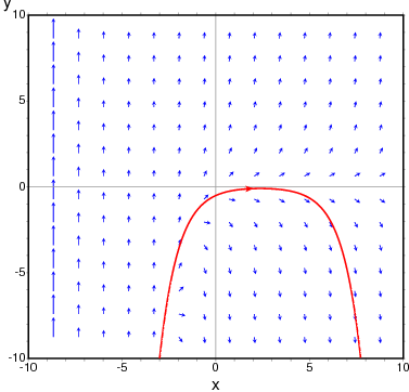
To obtain the direction field for the equation $dy/dx = x - y^2$
and the solution with initial condition $y(-1) = 3$, we can use the command:
maxima
(%i1) plotdf(x-y^2,[xfun,"sqrt(x);-sqrt(x)"],
         [trajectory_at,-1,3], [direction,forward],
         [y,-5,5], [x,-4,16])$
The graph also shows the function $y = \sqrt{x}.$
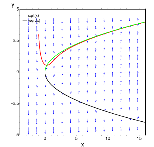
The following example shows the direction field of a harmonic oscillator, defined by the two equations $dz/dt = v$ and $dv/dt = -kz/m,$
and the integral curve through $(z,v) = (6,0)$, with a slider that will allow you to change the value of $m$ interactively ($k$ is fixed at 2):
maxima
(%i1) plotdf([v,-k*z/m], [z,v], [parameters,"m=2,k=2"],
           [sliders,"m=1:5"], [trajectory_at,6,0])$
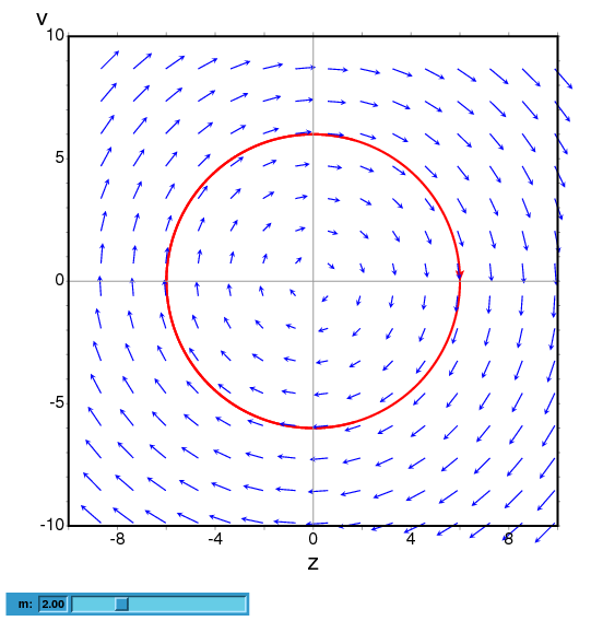
To plot the direction field of the Duffing equation, $m x’‘+c x’ + kx + bx^3 = 0,$ we introduce the variable $y=x’$ and use:
maxima
(%i1) plotdf([y,-(k*x + c*y + b*x^3)/m],
             [parameters,"k=-1,m=1.0,c=0,b=1"],
             [sliders,"k=-2:2,m=-1:1"],[tstep,0.1])$
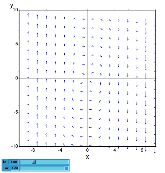
The direction field for a damped pendulum, including the solution for the given initial conditions, with a slider that can be used to change the value of the mass $m$, and with a plot of the two state variables as a function of time:
maxima
(%i1) plotdf([w,-g*sin(a)/l - b*w/m/l], [a,w],
        [parameters,"g=9.8,l=0.5,m=0.3,b=0.05"],
        [trajectory_at,1.05,-9],[tstep,0.01],
        [a,-10,2], [w,-14,14], [direction,forward],
        [nsteps,300], [sliders,"m=0.1:1"], [versus_t,1])$
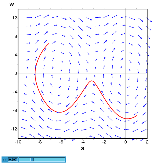
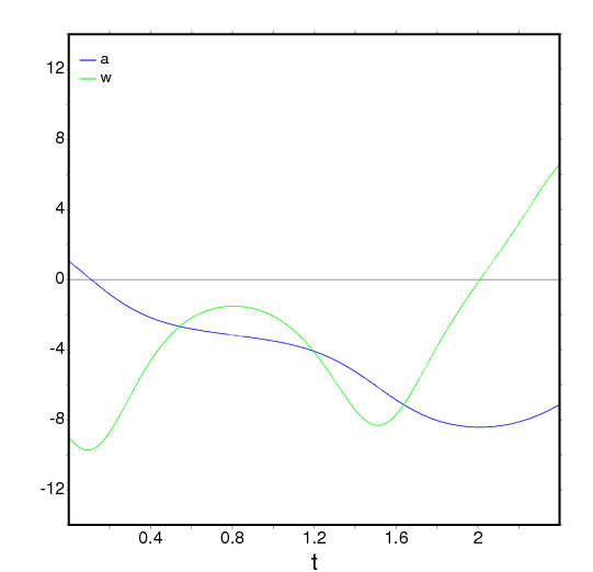
ploteq (exp, …options…) — Function
Plots equipotential curves for exp, which should be an expression depending on two variables. The curves are obtained by integrating the differential equation that define the orthogonal trajectories to the solutions of the autonomous system obtained from the gradient of the expression given. The plot can also show the integral curves for that gradient system (option fieldlines).
This program also requires Xmaxima, even if its run from a Maxima session in a console, since the plot will be created by the Tk scripts in Xmaxima. By default, the plot region will be empty until the user clicks in a point (or gives its coordinate with in the set-up menu or via the trajectory_at option).
Most options accepted by plotdf can also be used for ploteq and the plot interface is the same that was described in plotdf.
Example:
maxima
(%i1) V: 900/((x+1)^2+y^2)^(1/2)-900/((x-1)^2+y^2)^(1/2)$
(%i2) ploteq(V,[x,-2,2],[y,-2,2],[fieldlines,"blue"])$
Clicking on a point will plot the equipotential curve that passes by that point (in red) and the orthogonal trajectory (in blue).
rk (ODE, var, initial, domain) — Function
The first form solves numerically one first-order ordinary differential equation, and the second form solves a system of m of those equations, using the 4th order Runge-Kutta method. var represents the dependent variable. ODE must be an expression that depends only on the independent and dependent variables and defines the derivative of the dependent variable with respect to the independent variable.
The independent variable is specified with domain, which must be a
list of four elements as, for instance:
[t, 0, 10, 0.1]
the first element of the list identifies the independent variable, the second and third elements are the initial and final values for that variable, and the last element sets the increments that should be used within that interval.
If m equations are going to be solved, there should be m
dependent variables v1, v2, …, vm. The initial values
for those variables will be init1, init2, …, initm.
There will still be just one independent variable defined by domain,
as in the previous case. ODE1, …, ODEm are the expressions
that define the derivatives of each dependent variable in
terms of the independent variable. The only variables that may appear in
those expressions are the independent variable and any of the dependent
variables. It is important to give the derivatives ODE1, …,
ODEm in the list in exactly the same order used for the dependent
variables; for instance, the third element in the list will be interpreted
as the derivative of the third dependent variable.
The program will try to integrate the equations from the initial value of the independent variable until its last value, using constant increments. If at some step one of the dependent variables takes an absolute value too large, the integration will be interrupted at that point. The result will be a list with as many elements as the number of iterations made. Each element in the results list is itself another list with m+1 elements: the value of the independent variable, followed by the values of the dependent variables corresponding to that point.
See also drawdf, rk_adaptive, desolve and
ode2.
Examples:
To solve numerically the differential equation
$${{dx}\over{dt}} = t - x^2$$
$${{dx}\over{dt}} = t - x^2$$
With initial value $x(t=0) = 1$, in the interval of $t$ from 0 to 8 and with increments of 0.1 for $t$, use:
maxima
(%i1) results: rk(t-x^2,x,1,[t,0,8,0.1])$
(%i2) plot2d ([discrete, results])$
The results will be saved in the list results and the plot will show the solution obtained, with t on the horizontal axis and x on the vertical axis.
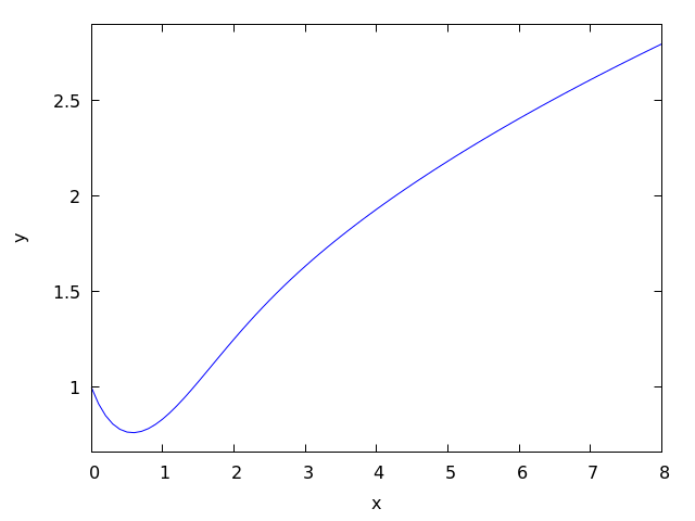
To solve numerically the system:
$$\eqalign{ {dx\over dy} &= 4-x^2-4y^2 \cr {dy\over dt} &= y^2 - x^2 + 1 }$$
$$\eqalign{ {dx\over dy} &= 4-x^2-4y^2 \cr {dy\over dt} &= y^2 - x^2 + 1 }$$
for $t$ between 0 and 4, and with values of -1.25 and 0.75 for $x$ and $y$ at $t=0$:
maxima

(%i1) sol: rk([4-x^2-4*y^2, y^2-x^2+1], [x, y], [-1.25, 0.75],
              [t,0,4,0.02])$


(%i2) plot2d([discrete, makelist([p[1], p[3]], p, sol)], [xlabel, "t"],
             [ylabel, "y"])$
The plot will show the solution for variable y as a function of t.
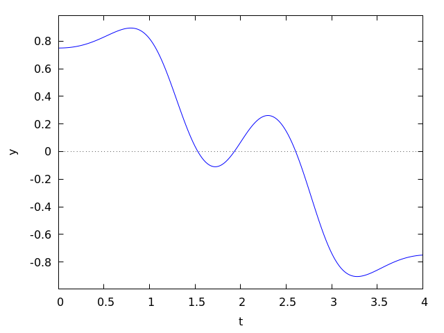
See also: drawdf, rk_adaptive, desolve, ode2.
Special Functions
expintegral_chi (z) — Function
The Exponential Integral Chi(z) (https://personal.math.ubc.ca/~cbm/aands/page_231.htmA&S eqn 5.2.4 and https://dlmf.nist.gov/6.2#E16DLMF 6.2#E16) defined as
$${\rm Chi}(z) = \gamma + \log z + \int_0^z {{\cosh t - 1} \over t} dt$$
$${\rm Chi}(z) = \gamma + \log z + \int_0^z {{\cosh t - 1} \over t} dt$$
with $|\arg z| < \pi.$
This can be written in terms of other functions. expintrep for examples.
See also: expintrep.
expintegral_ci (z) — Function
The Exponential Integral Ci(z) (https://personal.math.ubc.ca/~cbm/aands/page_231.htmA&S eqn 5.2.2 and https://dlmf.nist.gov/6.2#E13DLMF 6.2#E13) defined as
$${\rm Ci}(z) = \gamma + \log z + \int_0^z {{\cos t - 1} \over t} dt$$
$${\rm Ci}(z) = \gamma + \log z + \int_0^z {{\cos t - 1} \over t} dt$$
with $|\arg z| < \pi.$
This can be written in terms of other functions. expintrep for examples.
See also: expintrep.
expintegral_e (n, z) — Function
The Exponential Integral En(z) (https://personal.math.ubc.ca/~cbm/aands/page_228.htmA&S eqn 5.1.4) defined as
$$E_n(z) = \int_1^\infty {e^{-zt} \over t^n} dt$$
$$E_n(z) = \int_1^\infty {e^{-zt} \over t^n} dt$$
with ${\rm Re}(z) > 1$ and $n$ a non-negative integer.
For half-integral orders, this can be written in terms of erfc
or erf. expintexpand for examples.
See also: erfc, erf, expintexpand.
expintegral_e1 (z) — Function
The Exponential Integral E1(z) defined as
$$E_1(z) = \int_z^\infty {e^{-t} \over t} dt$$
$$E_1(z) = \int_z^\infty {e^{-t} \over t} dt$$
with $\left| \arg z \right| < \pi.$ (https://personal.math.ubc.ca/~cbm/aands/page_228.htmA&S eqn 5.1.1) and (https://dlmf.nist.gov/6.2E2DLMF 6.2E2)
This can be written in terms of other functions. expintrep for examples.
See also: expintrep.
expintegral_ei (x) — Function
The Exponential Integral Ei(x) defined as
$$Ei(x) = - -\kern-10.5pt\int_{-x}^\infty {e^{-t} \over t} dt = -\kern-10.5pt\int_{-\infty}^x {e^{t} \over t} dt$$
$$Ei(x) = - -\kern-10.5pt\int_{-x}^\infty {e^{-t} \over t} dt = -\kern-10.5pt\int_{-\infty}^x {e^{t} \over t} dt $$
with $x$ real and $x > 0$. (https://personal.math.ubc.ca/~cbm/aands/page_228.htmA&S eqn 5.1.2) and (https://dlmf.nist.gov/6.2E5DLMF 6.2E5)
This can be written in terms of other functions. expintrep for examples.
See also: expintrep.
expintegral_li (x) — Function
The Exponential Integral li(x) defined as
$$li(x) = -\kern-10.5pt\int_0^x {dt \over \ln t}$$
$$li(x) = -\kern-10.5pt\int_0^x {dt \over \ln t}$$
with $x$ real and $x > 1$. (https://personal.math.ubc.ca/~cbm/aands/page_228.htmA&S eqn 5.1.3) and (https://dlmf.nist.gov/6.2E8DLMF 6.2E8)
This can be written in terms of other functions. expintrep for examples.
See also: expintrep.
expintegral_shi (z) — Function
The Exponential Integral Shi(z) (https://personal.math.ubc.ca/~cbm/aands/page_231.htmA&S eqn 5.2.3 and https://dlmf.nist.gov/6.2#E15DLMF 6.2#E15) defined as
$${\rm Shi}(z) = \int_0^z {\sinh t \over t} dt$$
$${\rm Shi}(z) = \int_0^z {\sinh t \over t} dt$$
This can be written in terms of other functions. expintrep for examples.
See also: expintrep.
expintegral_si (z) — Function
The Exponential Integral Si(z) (https://personal.math.ubc.ca/~cbm/aands/page_231.htmA&S eqn 5.2.1 and https://dlmf.nist.gov/6.2#E9DLMF 6.2#E9) defined as
$${\rm Si}(z) = \int_0^z {\sin t \over t} dt$$
$${\rm Si}(z) = \int_0^z {\sin t \over t} dt$$
This can be written in terms of other functions. expintrep for examples.
See also: expintrep.
expintexpand — Variable
Default value: false
Expand expintegral_005fe for half
integral values in terms of erfc or erf and
for positive integers in terms of expintegral_ei.
maxima

(%i1) expintegral_e(1/2,z);
                                     1
(%o1)                  expintegral_e(-, z)
                                     2


(%i2) expintegral_e(1,z);
(%o2)                  expintegral_e(1, z)


(%i3) expintexpand:true;
(%o3)                         true


(%i4) expintegral_e(1/2,z);
                     sqrt(%pi) erfc(sqrt(z))
(%o4)                -----------------------
                             sqrt(z)


(%i5) expintegral_e(1,z);
                       1
                 log(- -) - log(- z)
                       z
(%o5) - log(z) - ------------------- - expintegral_ei(- z)
                          2
See also: expintegral_e, erfc, erf, expintegral_ei.
expintrep — Variable
Default value: false
Change the representation of one of the exponential integrals,
expintegral_005fe,
expintegral_005fe1, or
expintegral_005fei to an equivalent form if possible.
The possible values for expintrep are:
false — The representation is not changed.
gamma_incomplete — The representation uses gamma_incomplete.
expintegral_e1 — The representation uses expintegral_e1.
expintegral_ei — The representation uses expintegral_ei.
expintegral_li — The representation uses expintegral_li.
expintegral_trig — The representation uses expintegral_si or expintegral_ci.
expintegral_hyp — The representation uses expintegral_shi or expintegral_chi.
Here are some examples for expintrep set to
expintrep_002dgamma_002dincomplete:
maxima

(%i1) expintrep:'gamma_incomplete;
(%o1)                   gamma_incomplete


(%i2) expintegral_e1(z);
(%o2)                gamma_incomplete(0, z)


(%i3) expintegral_ei(z);
(%o3)     log(z) - log(- z) - gamma_incomplete(0, - z)


(%i4) expintegral_li(z);
(%o4) log(log(z)) - log(- log(z)) - gamma_incomplete(0, - log(z))


(%i5) expintegral_e(n,z);
                                            n - 1
(%o5)           gamma_incomplete(1 - n, z) z


(%i6) expintegral_si(z);
(%o6) (%i (- log(%i z) + log(- %i z) - gamma_incomplete(0, %i z)
                                + gamma_incomplete(0, - %i z)))/2


(%i7) expintegral_ci(z);
(%o7) log(z) - (log(%i z) + log(- %i z)
     + gamma_incomplete(0, %i z) + gamma_incomplete(0, - %i z))/2


(%i8) expintegral_shi(z);
(%o8) (log(z) - log(- z) + gamma_incomplete(0, z)
                                    - gamma_incomplete(0, - z))/2


(%i9) expintegral_chi(z);
(%o9) - (- log(z) + log(- z) + gamma_incomplete(0, z)
                                    + gamma_incomplete(0, - z))/2
For expintrep set to expintrep_002dexpintegral_002de1:
maxima

(%i1) expintrep:'expintegral_e1;
(%o1)                    expintegral_e1


(%i2) expintegral_ei(z);
(%o2)        log(z) - log(- z) - expintegral_e1(- z)


(%i3) expintegral_li(z);
(%o3) log(log(z)) - log(- log(z)) - expintegral_e1(- log(z))


(%i4) expintegral_e(n,z);
(%o4)                  expintegral_e(n, z)


(%i5) expintegral_si(z);
(%o5) (%i (- log(%i z) - expintegral_e1(%i z) + log(- %i z)
                                     + expintegral_e1(- %i z)))/2


(%i6) expintegral_ci(z);
(%o6) log(z) - (log(- %i z) (expintegral_e1(%i z)
                           + expintegral_e1(- %i z)) log(%i z))/2


(%i7) expintegral_shi(z);
      log(z) + expintegral_e1(z) - log(- z) - expintegral_e1(- z)
(%o7) -----------------------------------------------------------
                                   2


(%i8) expintegral_chi(z);
(%o8)
    - log(z) + expintegral_e1(z) + log(- z) + expintegral_e1(- z)
  - -------------------------------------------------------------
                                  2
For expintrep set to expintrep_002dexpintegral_002dei:
maxima

(%i1) expintrep:'expintegral_ei;
(%o1)                    expintegral_ei


(%i2) expintegral_e1(z);
                                  1
                 log(- z) - log(- -)
                                  z
(%o2) - log(z) + ------------------- - expintegral_ei(- z)
                          2


(%i3) expintegral_ei(z);
(%o3)                   expintegral_ei(z)


(%i4) expintegral_li(z);
(%o4)                expintegral_ei(log(z))


(%i5) expintegral_e(n,z);
(%o5)                  expintegral_e(n, z)


(%i6) expintegral_si(z);
(%o6) (%i (log(%i z) + 2 (expintegral_ei(- %i z)
                                              %i          %i
  - expintegral_ei(%i z)) - log(- %i z) + log(--) - log(- --)))/4
                                              z           z


(%i7) expintegral_ci(z);
(%o7) (- log(%i z) + 2 (expintegral_ei(%i z)
                                               %i          %i
 + expintegral_ei(- %i z)) - log(- %i z) + log(--) + log(- --))/4
                                               z           z
 + log(z)


(%i8) expintegral_shi(z);
(%o8) (- 2 log(z) + 2 (expintegral_ei(z) - expintegral_ei(- z))
                                                            1
                                         + log(- z) - log(- -))/4
                                                            z


(%i9) expintegral_chi(z);
(%o9) (2 log(z) + 2 (expintegral_ei(z) + expintegral_ei(- z))
                                                            1
                                         - log(- z) + log(- -))/4
                                                            z
For expintrep set to expintrep_002dexpintegral_002dli:
maxima

(%i1) expintrep:'expintegral_li;
(%o1)                    expintegral_li


(%i2) expintegral_e1(z);
                                                          1
                                         log(- z) - log(- -)
                         - z                              z
(%o2) - expintegral_li(%e   ) - log(z) + -------------------
                                                  2


(%i3) expintegral_ei(z);
                                        z
(%o3)                  expintegral_li(%e )


(%i4) expintegral_li(z);
(%o4)                   expintegral_li(z)


(%i5) expintegral_e(n,z);
(%o5)                  expintegral_e(n, z)


(%i6) expintegral_si(z);
                              %i z                     - %e z
(%o6) - (%i (expintegral_li(%e    ) - expintegral_li(%e      )
                                                %pi signum(z)
                                              - -------------))/2
                                                      2


(%i7) expintegral_ci(z);
                       %i z                     - %i z
      expintegral_li(%e    ) + expintegral_li(%e      )
(%o7) -------------------------------------------------
                              2
                                                  - signum(z) + 1


(%i8) expintegral_shi(z);
                            z                     - z
           expintegral_li(%e ) - expintegral_li(%e   )
(%o8)      -------------------------------------------
                                2


(%i9) expintegral_chi(z);
                            z                     - z
           expintegral_li(%e ) + expintegral_li(%e   )
(%o9)      -------------------------------------------
                                2
For expintrep set to expintrep_002dexpintegral_002dtrig:
maxima

(%i1) expintrep:'expintegral_trig;
(%o1)                   expintegral_trig


(%i2) expintegral_e1(z);
(%o2) log(%i z) - %i expintegral_si(%i z) - expintegral_ci(%i z)
                                                         - log(z)


(%i3) expintegral_ei(z);
(%o3) - log(%i z) - %i expintegral_si(%i z)
                                  + expintegral_ci(%i z) + log(z)


(%i4) expintegral_li(z);
(%o4) - log(%i log(z)) - %i expintegral_si(%i log(z))
                        + expintegral_ci(%i log(z)) + log(log(z))


(%i5) expintegral_e(n,z);
(%o5)                  expintegral_e(n, z)


(%i6) expintegral_si(z);
(%o6)                   expintegral_si(z)


(%i7) expintegral_ci(z);
(%o7)                   expintegral_ci(z)


(%i8) expintegral_shi(z);
(%o8)               - %i expintegral_si(%i z)


(%i9) expintegral_chi(z);
(%o9)      - log(%i z) + expintegral_ci(%i z) + log(z)
For expintrep set to expintrep_002dexpintegral_002dhyp:
maxima

(%i1) expintrep:'expintegral_hyp;
(%o1)                    expintegral_hyp


(%i2) expintegral_e1(z);
(%o2)        expintegral_shi(z) - expintegral_chi(z)


(%i3) expintegral_ei(z);
(%o3)        expintegral_shi(z) + expintegral_chi(z)


(%i4) expintegral_li(z);
(%o4)   expintegral_shi(log(z)) + expintegral_chi(log(z))


(%i5) expintegral_e(n,z);
(%o5)                  expintegral_e(n, z)


(%i6) expintegral_si(z);
(%o6)              - %i expintegral_shi(%i z)


(%i7) expintegral_ci(z);
(%o7)     - log(%i z) + expintegral_chi(%i z) + log(z)


(%i8) expintegral_shi(z);
(%o8)                  expintegral_shi(z)


(%i9) expintegral_chi(z);
(%o9)                  expintegral_chi(z)
See also: false, expintegral_e, expintegral_e1, expintegral_ei, expintrep, gamma_incomplete, expintegral_li, expintegral_si, expintegral_ci, expintegral_shi, expintegral_chi, expintrep-gamma-incomplete, expintrep-expintegral-e1, expintrep-expintegral-ei, expintrep-expintegral-li, expintrep-expintegral-trig, expintrep-expintegral-hyp.
bode
bode_gain (H, range, …plot_opts…) — Function
Function to draw Bode gain plots.
Examples (1 through 7 from
http://www.swarthmore.edu/NatSci/echeeve1/Ref/Bode/BodeHow.html,
8 from Ron Crummett):
(%i1) load("bode")$

(%i2) H1 (s) := 100 * (1 + s) / ((s + 10) * (s + 100))$

(%i3) bode_gain (H1 (s), [w, 1/1000, 1000])$

(%i4) H2 (s) := 1 / (1 + s/omega0)$

(%i5) bode_gain (H2 (s), [w, 1/1000, 1000]), omega0 = 10$

(%i6) H3 (s) := 1 / (1 + s/omega0)^2$

(%i7) bode_gain (H3 (s), [w, 1/1000, 1000]), omega0 = 10$

(%i8) H4 (s) := 1 + s/omega0$

(%i9) bode_gain (H4 (s), [w, 1/1000, 1000]), omega0 = 10$

(%i10) H5 (s) := 1/s$

(%i11) bode_gain (H5 (s), [w, 1/1000, 1000])$

(%i12) H6 (s) := 1/((s/omega0)^2 + 2 * zeta * (s/omega0) + 1)$

(%i13) bode_gain (H6 (s), [w, 1/1000, 1000]),
                  omega0 = 10, zeta = 1/10$

(%i14) H7 (s) := (s/omega0)^2 + 2 * zeta * (s/omega0) + 1$

(%i15) bode_gain (H7 (s), [w, 1/1000, 1000]),
                  omega0 = 10, zeta = 1/10$

(%i16) H8 (s) := 0.5 / (0.0001 * s^3 + 0.002 * s^2 + 0.01 * s)$

(%i17) bode_gain (H8 (s), [w, 1/1000, 1000])$
To use this function write first load("bode"). See also bode_005fphase.
See also: bode_phase.
bode_phase (H, range, …plot_opts…) — Function
Function to draw Bode phase plots.
Examples (1 through 7 from
http://www.swarthmore.edu/NatSci/echeeve1/Ref/Bode/BodeHow.html,
8 from Ron Crummett):
(%i1) load("bode")$

(%i2) H1 (s) := 100 * (1 + s) / ((s + 10) * (s + 100))$

(%i3) bode_phase (H1 (s), [w, 1/1000, 1000])$

(%i4) H2 (s) := 1 / (1 + s/omega0)$

(%i5) bode_phase (H2 (s), [w, 1/1000, 1000]), omega0 = 10$

(%i6) H3 (s) := 1 / (1 + s/omega0)^2$

(%i7) bode_phase (H3 (s), [w, 1/1000, 1000]), omega0 = 10$

(%i8) H4 (s) := 1 + s/omega0$

(%i9) bode_phase (H4 (s), [w, 1/1000, 1000]), omega0 = 10$

(%i10) H5 (s) := 1/s$

(%i11) bode_phase (H5 (s), [w, 1/1000, 1000])$

(%i12) H6 (s) := 1/((s/omega0)^2 + 2 * zeta * (s/omega0) + 1)$

(%i13) bode_phase (H6 (s), [w, 1/1000, 1000]),
                   omega0 = 10, zeta = 1/10$

(%i14) H7 (s) := (s/omega0)^2 + 2 * zeta * (s/omega0) + 1$

(%i15) bode_phase (H7 (s), [w, 1/1000, 1000]),
                   omega0 = 10, zeta = 1/10$

(%i16) H8 (s) := 0.5 / (0.0001 * s^3 + 0.002 * s^2 + 0.01 * s)$

(%i17) bode_phase (H8 (s), [w, 1/1000, 1000])$

(%i18) block ([bode_phase_unwrap : false],
              bode_phase (H8 (s), [w, 1/1000, 1000]));

(%i19) block ([bode_phase_unwrap : true],
              bode_phase (H8 (s), [w, 1/1000, 1000]));
To use this function write first load("bode"). See also bode_005fgain.
See also: bode_gain.
contrib_ode
bessel_simplify (expr) — Function
Simplifies expressions containing Bessel functions bessel_j,
bessel_y, bessel_i, bessel_k,
hankel_1, hankel_2, struve_h
and struve_005fl.
Recurrence relations https://personal.math.ubc.ca/~cbm/aands/page_361.htmA&S eqn 9.1.27 and https://dlmf.nist.gov/10.6#iDLMF 10.6#i
are used to replace functions of highest order n by functions of order n-1 and n-2.
This process is repeated until all the orders differ by less than 2.
(%i1) load("contrib_ode")$

(%i2) bessel_simplify(4*bessel_j(n,x^2)*(x^2-n^2/x^2)
  +x*((bessel_j(n-2,x^2)-bessel_j(n,x^2))*x
  -(bessel_j(n,x^2)-bessel_j(n+2,x^2))*x)
  -2*bessel_j(n+1,x^2)+2*bessel_j(n-1,x^2));
(%o2)                           0


(%i3) bessel_simplify( -2*bessel_j(1,z)*z^3 - 10*bessel_j(2,z)*z^2
 + 15*%pi*bessel_j(1,z)*struve_h(3,z)*z - 15*%pi*struve_h(1,z)
   *bessel_j(3,z)*z - 15*%pi*bessel_j(0,z)*struve_h(2,z)*z
 + 15*%pi*struve_h(0,z)*bessel_j(2,z)*z - 30*%pi*bessel_j(1,z)
   *struve_h(2,z) + 30*%pi*struve_h(1,z)*bessel_j(2,z));
(%o3)                           0
See also: bessel_j, bessel_y, bessel_i, bessel_k, hankel_1, hankel_2, struve_h, struve_l.
contrib_ode (eqn, y, x) — Function
Returns a list of solutions of the ODE eqn with independent variable x and dependent variable y.
dgauss_a (a, b, c, x) — Function
The derivative with respect to x
of gauss_a``(a, b, c, x).
See also: gauss_a.
dgauss_b (a, b, c, x) — Function
The derivative with respect to x
of gauss_b``(a, b, c, x).
See also: gauss_b.
dkummer_m (a, b, x) — Function
The derivative with respect to x
of kummer_m``(a, b, x).
See also: kummer_m.
dkummer_u (a, b, x) — Function
The derivative with respect to x
of kummer_u``(a, b, x).
See also: kummer_u.
expintegral_e_simplify (expr) — Function
Simplify expressions containing exponential integral expintegral_e
using the recurrence https://personal.math.ubc.ca/~cbm/aands/page_229.htmA&S eqn 5.1.14.
expintegral_e(n+1,z) = (1/n) * (exp(-z)-z*expintegral_e(n,z)) n = 1,2,3 ….
See also: expintegral_e.
gauss_a (a, b, c, x) — Function
gauss_a(a,b,c,x) and gauss_b(a,b,c,x) are 2F1
hypergeometric functions. They represent any two independent
solutions of the hypergeometric differential equation
x*(1-x) diff(y,x,2) + [c-(a+b+1)x] diff(y,x) - a*b*y = 0
See https://personal.math.ubc.ca/~cbm/aands/page_562.htmA&S eqn 15.5.1 and https://dlmf.nist.gov/15.10DLMF 15.10.
The only use of these functions is in solutions of ODEs returned by
odelin and contrib_ode. The definition and use of these
functions may change in future releases of Maxima.
See also gauss_b, dgauss_a and gauss_005fb.
See also: odelin, contrib_ode, gauss_b, dgauss_a.
gauss_b (a, b, c, x) — Function
See gauss_005fa.
See also: gauss_a.
kummer_m (a, b, x) — Function
Kummer’s M function, see https://personal.math.ubc.ca/~cbm/aands/page_504.htmA&S eqn 13.1.2 and https://dlmf.nist.gov/13.2DLMF 13.2.
The only use of this function is in solutions of ODEs returned by
odelin and contrib_ode. The definition and use of this
function may change in future releases of Maxima.
See also kummer_u, dkummer_m, and dkummer_005fu.
See also: odelin, contrib_ode, kummer_u, dkummer_m, dkummer_u.
kummer_u (a, b, x) — Function
Kummer’s U function, see https://personal.math.ubc.ca/~cbm/aands/page_504.htmA&S eqn 13.1.3 and https://dlmf.nist.gov/13.2.6DLMF 13.2.6.
See kummer_005fm.
See also: kummer_m.
ode_check (eqn, soln) — Function
Returns the value of ODE eqn after substituting a possible solution soln. The value is equivalent to zero if soln is a solution of eqn.
(%i1) load("contrib_ode")$

(%i2) eqn:'diff(y,x,2)+(a*x+b)*y;
                         2
                        d y
(%o2)                   --- + (b + a x) y
                          2
                        dx

(%i3) ans:[y = bessel_y(1/3,2*(a*x+b)^(3/2)/(3*a))*%k2*sqrt(a*x+b)
         +bessel_j(1/3,2*(a*x+b)^(3/2)/(3*a))*%k1*sqrt(a*x+b)];
                                  3/2
                    1  2 (b + a x)
(%o3) [y = bessel_y(-, --------------) %k2 sqrt(a x + b)
                    3       3 a
                                          3/2
                            1  2 (b + a x)
                 + bessel_j(-, --------------) %k1 sqrt(a x + b)]
                            3       3 a

(%i4) ode_check(eqn,ans[1]);
(%o4)                           0
odelin (eqn, y, x) — Function
odelin solves linear homogeneous ODEs of first and
second order with
independent variable x and dependent variable y.
It returns a fundamental solution set of the ODE.
For second order ODEs, odelin uses a method, due to Bronstein
and Lafaille, that searches for solutions in terms of given
special functions.
(%i1) load("contrib_ode")$

(%i2) odelin(x*(x+1)*'diff(y,x,2)+(x+5)*'diff(y,x,1)+(-4)*y,y,x);
       gauss_a(- 6, - 2, - 3, - x)  gauss_b(- 6, - 2, - 3, - x)
(%o2) {---------------------------, ---------------------------}
                    4                            4
                   x                            x
odepack
dlsode_init (fex, vars, method) — Function
This must be called before running the solver. This function returns a state object for use in the solver. The user must not modify the state.
The ODE to be solved is given in fex, which is a list of the equations. vars is a list of independent variable and the dependent variables. The list of dependent variables must be in the same order as the equations if fex. Finally, method indicates the method to be used by the solver:
10 — Nonstiff (Adams) method, no Jacobian used. 21 — Stiff (BDF) method, user-supplied full Jacobian. 22 — Stiff method, internally generated full Jacobian.
The returned state object is a list of lists. The sublist is a list of two elements:
f — The compiled function for the ODE. vars — The list independent and dependent variables (vars). mf — The method to be used (method). neq — The number of equations. lrw — Length of the work vector for real values. liw — Length of the work vector for integer values. rwork — Lisp array holding the real-valued work vector. iwork — Lisp array holding the integer-valued work vector. fjac — Compiled analytical Jacobian of the equations
See also dlsode_005fstep. Getting-Started-with-ODEPACK for
an example of usage.
See also: dlsode_step, Getting-Started-with-ODEPACK.
dlsode_step (inity, t, tout, rtol, atol, istate, state) — Function
Performs one step of the solver, returning the values of the independent and dependent variables, a success or error code.
The parameters for dlsode_step are:
inity — For the first call (when istate = 1), the initial values t — Current value of the independent value tout — Next point where output is desired which must not be equal to t. rtol — relative tolerance parameter atol — Absolute tolerance parameter, scalar of vector. If scalar, it applies to all dependent variables. Otherwise it must be the tolerance for each dependent variable. Use rtol = 0 for pure absolute error and use atol = 0 for pure relative error. istate — 1 for the first call to dlsode, 2 for subsequent calls. state — state returned by dlsode_init.
The output is a list of the following items:
t — independent variable value y — list of values of the dependent variables at time t. istate — Integration status: > 1 — no work because tout = tt
2 — successful result -1 — Excess work done on this call -2 — Excess accuracy requested -3 — Illegal input detected -4 — Repeated error test failures -5 — Repeated convergence failures (perhaps bad Jacobian or wrong choice of mf or tolerances) -6 — Error weight because zero during problem (solution component is vanished and atol(i) = 0. info — association list of various bits of information: > n_steps — total steps taken thus far n_f_eval — total number of function evals n_j_eval — total number of Jacobian evals method_order — method order len_rwork — Actual length used for real work array len_iwork — Actual length used for integer work array
See also dlsode_005finit. Getting-Started-with-ODEPACK for
an example of usage.
See also: dlsode_init, Getting-Started-with-ODEPACK.
romberg
romberg (expr, x, a, b) — Function
Computes a numerical integration by Romberg’s method.
romberg(expr, x, a, b)
returns an estimate of the integral integrate(expr, x, a, b).
expr must be an expression which evaluates to a floating point value
when x is bound to a floating point value.
romberg(F, a, b)
returns an estimate of the integral integrate(F(x), x, a, b)
where x represents the unnamed, sole argument of F;
the actual argument is not named x.
F must be a Maxima or Lisp function which returns a floating point value
when the argument is a floating point value.
F may name a translated or compiled Maxima function.
The accuracy of romberg is governed by the global variables
rombergabs and rombergtol.
romberg terminates successfully when
the absolute difference between successive approximations is less than rombergabs,
or the relative difference in successive approximations is less than rombergtol.
Thus when rombergabs is 0.0 (the default)
only the relative error test has any effect on romberg.
romberg halves the stepsize at most rombergit times before it gives up;
the maximum number of function evaluations is therefore 2^rombergit.
If the error criterion established by rombergabs and rombergtol
is not satisfied, romberg prints an error message.
romberg always makes at least rombergmin iterations;
this is a heuristic intended to prevent spurious termination when the integrand is oscillatory.
romberg repeatedly evaluates the integrand after binding the variable
of integration to a specific value (and not before).
This evaluation policy makes it possible to nest calls to romberg,
to compute multidimensional integrals.
However, the error calculations do not take the errors of nested integrations
into account, so errors may be underestimated.
Also, methods devised especially for multidimensional problems may yield
the same accuracy with fewer function evaluations.
See also Introduction to QUADPACK, a collection of numerical integration functions.
Examples:
A 1-dimensional integration.
(%i1) f(x) := 1/((x - 1)^2 + 1/100) + 1/((x - 2)^2 + 1/1000)
              + 1/((x - 3)^2 + 1/200);
                    1                 1                1
(%o1) f(x) := -------------- + --------------- + --------------
                     2    1           2    1            2    1
              (x - 1)  + ---   (x - 2)  + ----   (x - 3)  + ---
                         100              1000              200


(%i2) rombergtol : 1e-6;
(%o2)                 9.999999999999999e-7


(%i3) rombergit : 15;
(%o3)                          15


(%i4) estimate : romberg (f(x), x, -5, 5);
(%o4)                   173.6730736617464


(%i5) exact : integrate (f(x), x, -5, 5);
        3/2          3/2      3/2          3/2
(%o5) 10    atan(7 10   ) + 10    atan(3 10   )
      3/2         9/2       3/2         5/2
 + 5 2    atan(5 2   ) + 5 2    atan(5 2   ) + 10 atan(60)
 + 10 atan(40)


(%i6) abs (estimate - exact) / exact, numer;
(%o6)                 7.552722451569877e-11
A 2-dimensional integration, implemented by nested calls to romberg.
(%i1) g(x, y) := x*y / (x + y);
                                    x y
(%o1)                   g(x, y) := -----
                                   x + y


(%i2) rombergtol : 1e-6;
(%o2)                 9.999999999999999e-7


(%i3) estimate : romberg (romberg (g(x, y), y, 0, x/2), x, 1, 3);
(%o3)                  0.8193023962835647


(%i4) assume (x > 0);
(%o4)                        [x > 0]


(%i5) integrate (integrate (g(x, y), y, 0, x/2), x, 1, 3);
                                           3
                                     2 log(-) - 1
                    9                      2        9
(%o5)      (- 9 log(-)) + 9 log(3) + ------------ + -
                    2                     6         2


(%i6) exact : radcan (%);
                    26 log(3) - 26 log(2) - 13
(%o6)             - --------------------------
                                3


(%i7) abs (estimate - exact) / exact, numer;
(%o7)                 1.371197987185102e-10
See also: Introduction-to-QUADPACK.
rombergabs — Variable
Default value: 0.0
The accuracy of romberg is governed by the global variables
rombergabs and rombergtol.
romberg terminates successfully when
the absolute difference between successive approximations is less than rombergabs,
or the relative difference in successive approximations is less than rombergtol.
Thus when rombergabs is 0.0 (the default)
only the relative error test has any effect on romberg.
See also rombergit and rombergmin.
See also: rombergit, rombergmin.
rombergit — Variable
Default value: 11
romberg halves the stepsize at most rombergit times before it gives up;
the maximum number of function evaluations is therefore 2^rombergit.
romberg always makes at least rombergmin iterations;
this is a heuristic intended to prevent spurious termination when the integrand is oscillatory.
See also rombergabs and rombergtol.
See also: rombergabs, rombergtol.
rombergmin — Variable
Default value: 0
romberg always makes at least rombergmin iterations;
this is a heuristic intended to prevent spurious termination when the integrand is oscillatory.
See also rombergit, rombergabs, and rombergtol.
See also: rombergit, rombergabs, rombergtol.
rombergtol — Variable
Default value: 1e-4
The accuracy of romberg is governed by the global variables
rombergabs and rombergtol.
romberg terminates successfully when
the absolute difference between successive approximations is less than rombergabs,
or the relative difference in successive approximations is less than rombergtol.
Thus when rombergabs is 0.0 (the default)
only the relative error test has any effect on romberg.
See also rombergit and rombergmin.
See also: rombergit, rombergmin.
Combinatorics
Elementary Functions
Function: !!
The double factorial operator.
For an integer, float, or rational number n, n!! evaluates to the
product n (n-2) (n-4) (n-6) ... (n - 2 (k-1)) where k is equal to
entier (n/2), that is, the largest integer less than or equal to
n/2. Note that this definition does not coincide with other published
definitions for arguments which are not integers.
For an even (or odd) integer n, n!! evaluates to the product of
all the consecutive even (or odd) integers from 2 (or 1) through n
inclusive.
For an argument n which is not an integer, float, or rational, n!!
yields a noun form genfact (n, n/2, 2).
binomial (x, y) — Function
The binomial coefficient x!/(y! (x - y)!).
If x and y are integers, then the numerical value of the binomial
coefficient is computed. If y, or x - y, is an integer, the
binomial coefficient is expressed as a polynomial.
Examples:
maxima

(%i1) binomial (11, 7);
(%o1)                          330


(%i2) 11! / 7! / (11 - 7)!;
(%o2)                          330


(%i3) binomial (x, 7);
        (x - 6) (x - 5) (x - 4) (x - 3) (x - 2) (x - 1) x
(%o3)   -------------------------------------------------
                              5040


(%i4) binomial (x + 7, x);
      (x + 1) (x + 2) (x + 3) (x + 4) (x + 5) (x + 6) (x + 7)
(%o4) -------------------------------------------------------
                               5040


(%i5) binomial (11, y);
(%o5)                    binomial(11, y)
factcomb (expr) — Function
Tries to combine the coefficients of factorials in expr
with the factorials themselves by converting, for example, (n + 1)*n!
into (n + 1)!.
sumsplitfact if set to false will cause minfactorial to be
applied after a factcomb.
Example:
maxima

(%i1) sumsplitfact;
(%o1)                         true


(%i2) (n + 1)*(n + 1)*n!;
                                  2
(%o2)                      (n + 1)  n!


(%i3) factcomb (%);
(%o3)                  (n + 2)! - (n + 1)!


(%i4) sumsplitfact: not sumsplitfact;
(%o4)                         false


(%i5) (n + 1)*(n + 1)*n!;
                                  2
(%o5)                      (n + 1)  n!


(%i6) factcomb (%);
(%o6)                 n (n + 1)! + (n + 1)!
See also: sumsplitfact, minfactorial.
factlim — Variable
Default value: 100000
factlim specifies the highest factorial which is
automatically expanded. If it is -1 then all integers are expanded.
Function: factorial
Represents the factorial function. Maxima treats factorial (x)
the same as x!.
For any complex number x, except for negative integers, x! is
defined as gamma(x+1).
For an integer x, x! simplifies to the product of the integers
from 1 to x inclusive. 0! simplifies to 1. For a real or complex
number in float or bigfloat precision x, x! simplifies to the
value of gamma (x+1). For x equal to n/2 where n is
an odd integer, x! simplifies to a rational factor times
sqrt (%pi) (since gamma (1/2) is equal to sqrt (%pi)).
The option variables factlim and gammalim control the numerical
evaluation of factorials for integer and rational arguments. The functions
minfactorial and factcomb simplifies expressions containing
factorials.
The functions gamma, bffac, and cbffac are
varieties of the gamma function. bffac and cbffac are called
internally by gamma to evaluate the gamma function for real and complex
numbers in bigfloat precision.
makegamma substitutes gamma for factorials and related functions.
Maxima knows the derivative of the factorial function and the limits for specific values like negative integers.
The option variable factorial_expand controls the simplification of
expressions like (n+x)!, where n is an integer.
See also binomial.
The factorial of an integer is simplified to an exact number unless the operand
is greater than factlim. The factorial for real and complex numbers is
evaluated in float or bigfloat precision.
maxima

(%i1) factlim : 10;
(%o1)                          10


(%i2) [0!, (7/2)!, 8!, 20!];
                     105 sqrt(%pi)
(%o2)            [1, -------------, 40320, 20!]
                          16


(%i3) [4,77!, (1.0+%i)!];
(%o3) [4, 77!, 0.3430658398165453 %i + 0.6529654964201667]


(%i4) [2.86b0!, (1.0b0+%i)!];
(%o4) [5.046635586910012b0, 3.430658398165454b-1 %i
                                          + 6.529654964201667b-1]
The factorial of a known constant, or general expression is not simplified. Even so it may be possible to simplify the factorial after evaluating the operand.
maxima

(%i1) [(%i + 1)!, %pi!, %e!, (cos(1) + sin(1))!];
(%o1)      [(%i + 1)!, %pi!, %e!, (sin(1) + cos(1))!]


(%i2) ev (%, numer, %enumer);
(%o2) [0.3430658398165453 %i + 0.6529654964201667,
         7.188082728976031, 4.260820476357003, 1.227580202486819]
Factorials are simplified, not evaluated.
Thus x! may be replaced even in a quoted expression.
maxima

(%i1) '([0!, (7/2)!, 4.77!, 8!, 20!]);
          105 sqrt(%pi)
(%o1) [1, -------------, 81.44668037931197, 40320,
               16
                                             2432902008176640000]
Maxima knows the derivative of the factorial function.
maxima

(%i1) diff(x!,x);
(%o1)                    x! psi (x + 1)
                               0
The option variable factorial_expand controls expansion and
simplification of expressions with the factorial function.
maxima

(%i1) (n+1)!/n!,factorial_expand:true;
(%o1)                         n + 1
See also: factlim, gammalim, minfactorial, factcomb, gamma, bffac, cbffac, makegamma, factorial_expand, binomial.
factorial_expand — Variable
Default value: false
The option variable factorial_expand controls the simplification of
expressions like (x+n)!, where n is an integer.
See factorial for an example.
See also: factorial.
genfact (x, y, z) — Function
Returns the generalized factorial, defined as
x (x-z) (x - 2 z) ... (x - (y - 1) z). Thus, when x is an integer,
genfact (x, x, 1) = x! and genfact (x, x/2, 2) = x!!.
When x and z are integers,
and floor(y) is an integer,
genfact(x, y, y) simplifies to a number.
minfactorial (expr) — Function
Examines expr for occurrences of two factorials
which differ by an integer.
minfactorial then turns one into a polynomial times the other.
maxima

(%i1) n!/(n+2)!;
                               n!
(%o1)                       --------
                            (n + 2)!


(%i2) minfactorial (%);
                                1
(%o2)                    ---------------
                         (n + 1) (n + 2)
sumsplitfact — Variable
Default value: true
When sumsplitfact is false,
minfactorial is applied after a factcomb.
maxima

(%i1) sumsplitfact;
(%o1)                         true


(%i2) n!/(n+2)!;
                               n!
(%o2)                       --------
                            (n + 2)!


(%i3) factcomb(%);
                               n!
(%o3)                       --------
                            (n + 2)!


(%i4) sumsplitfact: not sumsplitfact ;
(%o4)                         false


(%i5) n!/(n+2)!;
                               n!
(%o5)                       --------
                            (n + 2)!


(%i6) factcomb(%);
                                1
(%o6)                    ---------------
                         (n + 1) (n + 2)
See also: minfactorial, factcomb.
Sets
adjoin (x, a) — Function
Returns the union of the set a with {x}.
adjoin complains if a is not a literal set.
adjoin(x, a) and union(set(x), a)
are equivalent;
however, adjoin may be somewhat faster than union.
See also disjoin.
Examples:
maxima

(%i1) adjoin (c, {a, b});
(%o1)                       {a, b, c}


(%i2) adjoin (a, {a, b});
(%o2)                        {a, b}
See also: disjoin.
belln (n) — Function
Represents the $n$-th Bell number.
belln(n) is the number of partitions of a set with n members.
For nonnegative integers n,
belln(n) simplifies to the $n$-th Bell number.
belln does not simplify for any other arguments.
belln distributes over equations, lists, matrices, and sets.
Examples:
belln applied to nonnegative integers.
maxima

(%i1) makelist (belln (i), i, 0, 6);
(%o1)               [1, 1, 2, 5, 15, 52, 203]


(%i2) is (cardinality (set_partitions ({})) = belln (0));
(%o2)                         true


(%i3) is (cardinality (set_partitions ({1, 2, 3, 4, 5, 6})) =
                       belln (6));
(%o3)                         true
belln applied to arguments which are not nonnegative integers.
maxima

(%i1) [belln (x), belln (sqrt(3)), belln (-9)];
(%o1)        [belln(x), belln(sqrt(3)), belln(- 9)]
cardinality (a) — Function
Returns the number of distinct elements of the set a.
cardinality ignores redundant elements
even when simplification is disabled.
Examples:
maxima

(%i1) cardinality ({});
(%o1)                           0


(%i2) cardinality ({a, a, b, c});
(%o2)                           3


(%i3) simp : false;
(%o3)                         false


(%i4) cardinality ({a, a, b, c});
(%o4)                           3
cartesian_product (b_1, …, b_n) — Function
Returns a set of lists of the form [x_1, ..., x_n], where
x_1, …, x_n are elements of the sets b_1, … , b_n,
respectively.
cartesian_product complains if any argument is not a literal set.
See also cartesian_005fproduct_005flist.
Examples:
maxima

(%i1) cartesian_product ({0, 1});
(%o1)                      {[0], [1]}


(%i2) cartesian_product ({0, 1}, {0, 1});
(%o2)           {[0, 0], [0, 1], [1, 0], [1, 1]}


(%i3) cartesian_product ({x}, {y}, {z});
(%o3)                      {[x, y, z]}


(%i4) cartesian_product ({x}, {-1, 0, 1});
(%o4)              {[x, - 1], [x, 0], [x, 1]}
See also: cartesian_product_list.
cartesian_product_list (b_1, …, b_n) — Function
Returns a list of lists of the form [x_1, ..., x_n], where
x_1, …, x_n are elements of the lists b_1, … , b_n, respectively,
comprising all possible combinations of the elements of b_1, … , b_n.
The list returned by cartesian_product_list is equivalent to the
following recursive definition.
Let L be the list returned by cartesian_product_list(b_2, ..., b_n).
Then cartesian_product_list(b_1, b_2, ..., b_n)
(i.e., b_1 in addition to b_2, …, b_n)
returns a list comprising each element of L appended to the first element of b_1,
each element of L appended to the second element of b_1,
each element of L appended to the third element of b_1, etc.
The order of the list returned by cartesian_product_list(b_1, b_2, ..., b_n)
may therefore be summarized by saying the lesser indices (1, 2, 3, …) vary more slowly than the greater indices.
The list returned by cartesian_product_list contains duplicate elements
if any argument b_1, …, b_n contains duplicates.
In this respect, cartesian_product_list differs from cartesian_product,
which returns no duplicates.
Also, the ordering of the list returned cartesian_product_list
is determined by the order of the elements of b_1, …, b_n.
Again, this differs from cartesian_product,
which returns a set (with order determined by orderlessp).
The length of the list returned by cartesian_product_list
is equal to the product of the lengths of the arguments b_1, …, b_n.
See also cartesian_005fproduct.
cartesian_product_list complains if any argument is not a list.
Examples:
cartesian_product_list returns a list of lists comprising all possible combinations.
maxima

(%i1) cartesian_product_list ([0, 1]);
(%o1)                      [[0], [1]]


(%i2) cartesian_product_list ([0, 1], [0, 1]);
(%o2)           [[0, 0], [0, 1], [1, 0], [1, 1]]


(%i3) cartesian_product_list ([x], [y], [z]);
(%o3)                      [[x, y, z]]


(%i4) cartesian_product_list ([x], [-1, 0, 1]);
(%o4)              [[x, - 1], [x, 0], [x, 1]]


(%i5) cartesian_product_list ([a, h, e], [c, b, 4]);
(%o5) [[a, c], [a, b], [a, 4], [h, c], [h, b], [h, 4], [e, c],
                                                  [e, b], [e, 4]]
The order of the list returned by cartesian_product_list
may be summarized by saying the lesser indices vary more slowly than the greater indices.
maxima

(%i1) cartesian_product_list ([1, 2, 3], [a, b], [i, ii]);
(%o1) [[1, a, i], [1, a, ii], [1, b, i], [1, b, ii], [2, a, i],
[2, a, ii], [2, b, i], [2, b, ii], [3, a, i], [3, a, ii],
[3, b, i], [3, b, ii]]
The list returned by cartesian_product_list contains duplicate elements
if any argument contains duplicates.
maxima

(%i1) cartesian_product_list ([e, h], [3, 7, 3]);
(%o1)   [[e, 3], [e, 7], [e, 3], [h, 3], [h, 7], [h, 3]]
The length of the list returned by cartesian_product_list
is equal to the product of the lengths of the arguments.
maxima

(%i1) foo: cartesian_product_list ([1, 1, 2, 2, 3], [h, z, h]);
(%o1) [[1, h], [1, z], [1, h], [1, h], [1, z], [1, h], [2, h],
  [2, z], [2, h], [2, h], [2, z], [2, h], [3, h], [3, z], [3, h]]


(%i2) is (length (foo) = 5*3);
(%o2)                         true
See also: cartesian_product.
disjoin (x, a) — Function
Returns the set a without the member x. If x is not a member of a, return a unchanged.
disjoin complains if a is not a literal set.
disjoin(x, a), delete(x, a), and
setdifference(a, set(x)) are all equivalent.
Of these, disjoin is generally faster than the others.
Examples:
maxima

(%i1) disjoin (a, {a, b, c, d});
(%o1)                       {b, c, d}


(%i2) disjoin (a + b, {5, z, a + b, %pi});
(%o2)                      {5, %pi, z}


(%i3) disjoin (a - b, {5, z, a + b, %pi});
(%o3)                  {5, %pi, b + a, z}
disjointp (a, b) — Function
Returns true if and only if the sets a and b are disjoint.
disjointp complains if either a or b is not a literal set.
Examples:
maxima

(%i1) disjointp ({a, b, c}, {1, 2, 3});
(%o1)                         true


(%i2) disjointp ({a, b, 3}, {1, 2, 3});
(%o2)                         false
divisors (n) — Function
Represents the set of divisors of n.
divisors(n) simplifies to a set of integers
when n is a nonzero integer.
The set of divisors includes the members 1 and n.
The divisors of a negative integer are the divisors of its absolute value.
divisors distributes over equations, lists, matrices, and sets.
Examples:
We can verify that 28 is a perfect number: the sum of its divisors (except for itself) is 28.
maxima

(%i1) s: divisors(28);
(%o1)                 {1, 2, 4, 7, 14, 28}


(%i2) lreduce ("+", args(s)) - 28;
(%o2)                          28
divisors is a simplifying function.
Substituting 8 for a in divisors(a)
yields the divisors without reevaluating divisors(8).
maxima

(%i1) divisors (a);
(%o1)                      divisors(a)


(%i2) subst (8, a, %);
(%o2)                     {1, 2, 4, 8}
divisors distributes over equations, lists, matrices, and sets.
maxima

(%i1) divisors (a = b);
(%o1)               divisors(a) = divisors(b)


(%i2) divisors ([a, b, c]);
(%o2)        [divisors(a), divisors(b), divisors(c)]


(%i3) divisors (matrix ([a, b], [c, d]));
                  [ divisors(a)  divisors(b) ]
(%o3)             [                          ]
                  [ divisors(c)  divisors(d) ]


(%i4) divisors ({a, b, c});
(%o4)        {divisors(a), divisors(b), divisors(c)}
elementp (x, a) — Function
Returns true if and only if x is a member of the
set a.
elementp complains if a is not a literal set.
Examples:
maxima

(%i1) elementp (sin(1), {sin(1), sin(2), sin(3)});
(%o1)                         true


(%i2) elementp (sin(1), {cos(1), cos(2), cos(3)});
(%o2)                         false
emptyp (a) — Function
Return true if and only if a is the empty set or
the empty list.
Examples:
maxima

(%i1) map (emptyp, [{}, []]);
(%o1)                     [true, true]


(%i2) map (emptyp, [a + b, {{}}, %pi]);
(%o2)                 [false, false, false]
equiv_classes (s, F) — Function
Returns a set of the equivalence classes of the set s with respect to the equivalence relation F.
F is a function of two variables defined on the Cartesian product of s with s.
The return value of F is either true or false,
or an expression expr such that is(expr) is either true or false.
When F is not an equivalence relation,
equiv_classes accepts it without complaint,
but the result is generally incorrect in that case.
Examples:
The equivalence relation is a lambda expression which returns true or false.
maxima

(%i1) equiv_classes ({1, 1.0, 2, 2.0, 3, 3.0},
                        lambda ([x, y], is (equal (x, y))));
(%o1)            {{1, 1.0}, {2, 2.0}, {3, 3.0}}
The equivalence relation is the name of a relational function
which is evaluates to true or false.
maxima

(%i1) equiv_classes ({1, 1.0, 2, 2.0, 3, 3.0}, equal);
(%o1)            {{1, 1.0}, {2, 2.0}, {3, 3.0}}
The equivalence classes are numbers which differ by a multiple of 3.
maxima

(%i1) equiv_classes ({1, 2, 3, 4, 5, 6, 7},
                     lambda ([x, y], remainder (x - y, 3) = 0));
(%o1)              {{1, 4, 7}, {2, 5}, {3, 6}}
every (f, s) — Function
Returns true if the predicate f is true for all given arguments.
Given one set as the second argument,
every(f, s) returns true
if is(f(a_i)) returns true for all a_i in s.
every may or may not evaluate f for all a_i in s.
Since sets are unordered,
every may evaluate f(a_i) in any order.
Given one or more lists as arguments,
every(f, L_1, ..., L_n) returns true
if is(f(x_1, ..., x_n)) returns true
for all x_1, …, x_n in L_1, …, L_n, respectively.
every may or may not evaluate
f for every combination x_1, …, x_n.
every evaluates lists in the order of increasing index.
Given an empty set {} or empty lists [] as arguments,
every returns true.
When the global flag maperror is true, all lists
L_1, …, L_n must have equal lengths.
When maperror is false, list arguments are
effectively truncated to the length of the shortest list.
Return values of the predicate f which evaluate (via is)
to something other than true or false
are governed by the global flag prederror.
When prederror is true,
such values are treated as false,
and the return value from every is false.
When prederror is false,
such values are treated as unknown,
and the return value from every is unknown.
Examples:
every applied to a single set.
The predicate is a function of one argument.
maxima

(%i1) every (integerp, {1, 2, 3, 4, 5, 6});
(%o1)                         true


(%i2) every (atom, {1, 2, sin(3), 4, 5 + y, 6});
(%o2)                         false
every applied to two lists.
The predicate is a function of two arguments.
maxima

(%i1) every ("=", [a, b, c], [a, b, c]);
(%o1)                         true


(%i2) every ("#", [a, b, c], [a, b, c]);
(%o2)                         false
Return values of the predicate f which evaluate
to something other than true or false
are governed by the global flag prederror.
maxima

(%i1) prederror : false;
(%o1)                         false


(%i2) map (lambda ([a, b], is (a < b)), [x, y, z],
                   [x^2, y^2, z^2]);
(%o2)              [unknown, unknown, unknown]


(%i3) every ("<", [x, y, z], [x^2, y^2, z^2]);
(%o3)                        unknown


(%i4) prederror : true;
(%o4)                         true


(%i5) every ("<", [x, y, z], [x^2, y^2, z^2]);
(%o5)                         false
extremal_subset (s, f, max) — Function
Returns the subset of s for which the function f takes on maximum or minimum values.
extremal_subset(s, f, max) returns the subset of the set or
list s for which the real-valued function f takes on its maximum value.
extremal_subset(s, f, min) returns the subset of the set or
list s for which the real-valued function f takes on its minimum value.
Examples:
maxima

(%i1) extremal_subset ({-2, -1, 0, 1, 2}, abs, max);
(%o1)                       {- 2, 2}


(%i2) extremal_subset ({sqrt(2), 1.57, %pi/2}, sin, min);
(%o2)                       {sqrt(2)}
flatten (expr) — Function
Collects arguments of subexpressions which have the same operator as expr and constructs an expression from these collected arguments.
Subexpressions in which the operator is different from the main operator of expr
are copied without modification,
even if they, in turn, contain some subexpressions in which the operator is the same as for expr.
It may be possible for flatten to construct expressions in which the number
of arguments differs from the declared arguments for an operator;
this may provoke an error message from the simplifier or evaluator.
flatten does not try to detect such situations.
Expressions with special representations, for example, canonical rational expressions (CRE),
cannot be flattened; in such cases, flatten returns its argument unchanged.
Examples:
Applied to a list, flatten gathers all list elements that are lists.
maxima

(%i1) flatten ([a, b, [c, [d, e], f], [[g, h]], i, j]);
(%o1)            [a, b, c, d, e, f, g, h, i, j]
Applied to a set, flatten gathers all members of set elements that are sets.
maxima

(%i1) flatten ({a, {b}, {{c}}});
(%o1)                       {a, b, c}


(%i2) flatten ({a, {[a], {a}}});
(%o2)                       {a, [a]}
flatten is similar to the effect of declaring the main operator n-ary.
However, flatten has no effect on subexpressions which have an operator
different from the main operator, while an n-ary declaration affects those.
maxima

(%i1) expr: flatten (f (g (f (f (x)))));
(%o1)                     f(g(f(f(x))))


(%i2) declare (f, nary);
(%o2)                         done


(%i3) ev (expr);
(%o3)                     f(g(f(f(x))))
flatten treats subscripted functions the same as any other operator.
maxima

(%i1) flatten (f[5] (f[5] (x, y), z));
(%o1)                      f (x, y, z)
                            5
It may be possible for flatten to construct expressions in which the number
of arguments differs from the declared arguments for an operator;
mod: expected exactly 2 arguments but got 3: [5, 7, 4] – an error. To debug this try: debugmode(true);
maxima

(%i1) 'mod (5, 'mod (7, 4));
(%o1)                   mod(5, mod(7, 4))


(%i2) flatten (%);
(%o2)                     mod(5, 7, 4)

(%i3) ''%, nouns;
full_listify (a) — Function
Replaces every set operator in a by a list operator,
and returns the result.
full_listify replaces set operators in nested subexpressions,
even if the main operator is not set.
listify replaces only the main operator.
Examples:
maxima

(%i1) full_listify ({a, b, {c, {d, e, f}, g}});
(%o1)               [a, b, [c, [d, e, f], g]]


(%i2) full_listify (F (G ({a, b, H({c, d, e})})));
(%o2)              F(G([a, b, H([c, d, e])]))
fullsetify (a) — Function
When a is a list, replaces the list operator with a set operator,
and applies fullsetify to each member which is a set.
When a is not a list, it is returned unchanged.
setify replaces only the main operator.
Examples:
In line (%o2), the argument of f isn’t converted to a set
because the main operator of f([b]) isn’t a list.
maxima

(%i1) fullsetify ([a, [a]]);
(%o1)                       {a, {a}}


(%i2) fullsetify ([a, f([b])]);
(%o2)                      {a, f([b])}
identity (x) — Function
Returns x for any argument x.
Examples:
identity may be used as a predicate when the arguments
are already Boolean values.
maxima

(%i1) every (identity, [true, true]);
(%o1)                         true
integer_partitions (n) — Function
Returns integer partitions of n, that is, lists of integers which sum to n.
integer_partitions(n) returns the set of
all partitions of the integer n.
Each partition is a list sorted from greatest to least.
integer_partitions(n, len)
returns all partitions that have length len or less; in this
case, zeros are appended to each partition with fewer than len
terms to make each partition have exactly len terms.
Each partition is a list sorted from greatest to least.
A list $[a_1, …, a_m]$ is a partition of a nonnegative integer $n$ when (1) each $a_i$ is a nonzero integer, and (2) $a_1 + … + a_m = n.$ Thus 0 has no partitions.
Examples:
maxima

(%i1) integer_partitions (3);
(%o1)               {[1, 1, 1], [2, 1], [3]}

(%i2) s: integer_partitions (25)$

(%i3) cardinality (s);
(%o3)                         1958


(%i4) map (lambda ([x], apply ("+", x)), s);
(%o4)                         {25}


(%i5) integer_partitions (5, 3);
(%o5) {[2, 2, 1], [3, 1, 1], [3, 2, 0], [4, 1, 0], [5, 0, 0]}


(%i6) integer_partitions (5, 2);
(%o6)               {[3, 2], [4, 1], [5, 0]}
To find all partitions that satisfy a condition, use the function subset;
here is an example that finds all partitions of 10 that consist of prime numbers.
maxima
(%i1) s: integer_partitions (10)$

(%i2) cardinality (s);
(%o2)                          42

(%i3) xprimep(x) := integerp(x) and (x > 1) and primep(x)$

(%i4) subset (s, lambda ([x], every (xprimep, x)));
(%o4) {[2, 2, 2, 2, 2], [3, 3, 2, 2], [5, 3, 2], [5, 5], [7, 3]}
intersect (a_1, …, a_n) — Function
intersect is the same as intersection, which see.
intersection (a_1, …, a_n) — Function
Returns a set containing the elements that are common to the sets a_1 through a_n.
intersection complains if any argument is not a literal set.
Examples:
maxima

(%i1) S_1 : {a, b, c, d};
(%o1)                     {a, b, c, d}


(%i2) S_2 : {d, e, f, g};
(%o2)                     {d, e, f, g}


(%i3) S_3 : {c, d, e, f};
(%o3)                     {c, d, e, f}


(%i4) S_4 : {u, v, w};
(%o4)                       {u, v, w}


(%i5) intersection (S_1, S_2);
(%o5)                          {d}


(%i6) intersection (S_2, S_3);
(%o6)                       {d, e, f}


(%i7) intersection (S_1, S_2, S_3);
(%o7)                          {d}


(%i8) intersection (S_1, S_2, S_3, S_4);
(%o8)                          {}
kron_delta (x1, x2, …, xp) — Function
Represents the Kronecker delta function.
kron_delta simplifies to 1 when xi and yj are equal
for all pairs of arguments, and it simplifies to 0 when xi and
yj are not equal for some pair of arguments. Equality is
determined using is(equal(xi,xj)) and inequality by
is(notequal(xi,xj)). For exactly one argument, kron_delta
signals an error.
Examples:
maxima

(%i1) kron_delta(a,a);
(%o1)                           1


(%i2) kron_delta(a,b,a,b);
(%o2)                   kron_delta(a, b)


(%i3) kron_delta(a,a,b,a+1);
(%o3)                           0


(%i4) assume(equal(x,y));
(%o4)                     [equal(x, y)]


(%i5) kron_delta(x,y);
(%o5)                           1
listify (a) — Function
Returns a list containing the members of a when a is a set.
Otherwise, listify returns a.
full_listify replaces all set operators in a by list operators.
Examples:
maxima

(%i1) listify ({a, b, c, d});
(%o1)                     [a, b, c, d]


(%i2) listify (F ({a, b, c, d}));
(%o2)                    F({a, b, c, d})
makeset (expr, x, s) — Function
Returns a set with members generated from the expression expr, where x is a list of variables in expr, and s is a set or list of lists. To generate each set member, expr is evaluated with the variables x bound in parallel to a member of s.
Each member of s must have the same length as x. The list of variables x must be a list of symbols, without subscripts. Even if there is only one symbol, x must be a list of one element, and each member of s must be a list of one element.
See also makelist.
Examples:
maxima

(%i1) makeset (i/j, [i, j], [[1, a], [2, b], [3, c], [4, d]]);
                           1  2  3  4
(%o1)                     {-, -, -, -}
                           a  b  c  d

(%i2) S : {x, y, z}$

(%i3) S3 : cartesian_product (S, S, S);
(%o3) {[x, x, x], [x, x, y], [x, x, z], [x, y, x], [x, y, y],
[x, y, z], [x, z, x], [x, z, y], [x, z, z], [y, x, x],
[y, x, y], [y, x, z], [y, y, x], [y, y, y], [y, y, z],
[y, z, x], [y, z, y], [y, z, z], [z, x, x], [z, x, y],
[z, x, z], [z, y, x], [z, y, y], [z, y, z], [z, z, x],
[z, z, y], [z, z, z]}


(%i4) makeset (i + j + k, [i, j, k], S3);
(%o4) {3 x, 3 y, y + 2 x, 2 y + x, 3 z, z + 2 x, z + y + x,
                                       z + 2 y, 2 z + x, 2 z + y}


(%i5) makeset (sin(x), [x], {[1], [2], [3]});
(%o5)               {sin(1), sin(2), sin(3)}
See also: makelist.
moebius (n) — Function
Represents the Moebius function.
When n is product of $k$ distinct primes,
moebius(n) simplifies to $(-1)^k$;
when $n = 1$, it simplifies to 1;
and it simplifies to 0 for all other positive integers.
moebius distributes over equations, lists, matrices, and sets.
Examples:
maxima

(%i1) moebius (1);
(%o1)                           1


(%i2) moebius (2 * 3 * 5);
(%o2)                          - 1


(%i3) moebius (11 * 17 * 29 * 31);
(%o3)                           1


(%i4) moebius (2^32);
(%o4)                           0


(%i5) moebius (n);
(%o5)                      moebius(n)


(%i6) moebius (n = 12);
(%o6)                    moebius(n) = 0


(%i7) moebius ([11, 11 * 13, 11 * 13 * 15]);
(%o7)                      [- 1, 1, 1]


(%i8) moebius (matrix ([11, 12], [13, 14]));
                           [ - 1  0 ]
(%o8)                      [        ]
                           [ - 1  1 ]


(%i9) moebius ({21, 22, 23, 24});
(%o9)                      {- 1, 0, 1}
multinomial_coeff (a_1, …, a_n) — Function
Returns the multinomial coefficient.
When each a_k is a nonnegative integer, the multinomial coefficient
gives the number of ways of placing a_1 + ... + a_n
distinct objects into $n$ boxes with a_k elements in the
$k$’th box. In general, multinomial_coeff (a_1, ..., a_n)
evaluates to (a_1 + ... + a_n)!/(a_1! ... a_n!).
multinomial_coeff() (with no arguments) evaluates to 1.
minfactorial may be able to simplify the value returned by multinomial_coeff.
Examples:
factorial: factorial of negative integer -6 not defined. – an error. To debug this try: debugmode(true);
maxima

(%i1) multinomial_coeff (1, 2, x);
                            (x + 3)!
(%o1)                       --------
                              2 x!


(%i2) minfactorial (%);
                     (x + 1) (x + 2) (x + 3)
(%o2)                -----------------------
                                2

(%i3) multinomial_coeff (-6, 2);

(%i4) minfactorial (%);
                     (x + 1) (x + 2) (x + 3)
(%o4)                -----------------------
                                2
num_distinct_partitions (n) — Function
Returns the number of distinct integer partitions of n
when n is a nonnegative integer.
Otherwise, num_distinct_partitions returns a noun expression.
num_distinct_partitions(n, list) returns a
list of the number of distinct partitions of 1, 2, 3, …, n.
A distinct partition of n is a list of distinct positive integers $k_1$, …, $k_m$ such that $n = k_1 + … + k_m$.
Examples:
maxima

(%i1) num_distinct_partitions (12);
(%o1)                          15


(%i2) num_distinct_partitions (12, list);
(%o2)        [1, 1, 2, 2, 3, 4, 5, 6, 8, 10, 12, 15]


(%i3) num_distinct_partitions (n);
(%o3)              num_distinct_partitions(n)
num_partitions (n) — Function
Returns the number of integer partitions of n
when n is a nonnegative integer.
Otherwise, num_partitions returns a noun expression.
num_partitions(n, list) returns a
list of the number of integer partitions of 1, 2, 3, …, n.
For a nonnegative integer n, num_partitions(n) is equal to
cardinality(integer_partitions(n)); however, num_partitions
does not actually construct the set of partitions, so it is much faster.
Examples:
maxima

(%i1) num_partitions (5) = cardinality (integer_partitions (5));
(%o1)                         7 = 7


(%i2) num_partitions (8, list);
(%o2)              [1, 2, 3, 5, 7, 11, 15, 22]


(%i3) num_partitions (n);
(%o3)                   num_partitions(n)
partition_set (a, f) — Function
Partitions the set a according to the predicate f.
partition_set returns a list of two sets.
The first set comprises the elements of a for which f evaluates to false,
and the second comprises any other elements of a.
partition_set does not apply is to the return value of f.
partition_set complains if a is not a literal set.
See also subset.
Examples:
maxima

(%i1) partition_set ({2, 7, 1, 8, 2, 8}, evenp);
(%o1)                   [{1, 7}, {2, 8}]


(%i2) partition_set ({x, rat(y), rat(y) + z, 1},
                     lambda ([x], ratp(x)));
(%o2)/R/              [{1, x}, {y, y + z}]
See also: subset.
permutations (a) — Function
Returns a set of all distinct permutations of the members of the list or set a. Each permutation is a list, not a set.
When a is a list, duplicate members of a are included in the permutations.
permutations complains if a is not a literal list or set.
See also random_permutation.
Examples:
maxima

(%i1) permutations ([a, a]);
(%o1)                       {[a, a]}


(%i2) permutations ([a, a, b]);
(%o2)           {[a, a, b], [a, b, a], [b, a, a]}
See also: random_permutation.
powerset (a) — Function
Returns the set of all subsets of a, or a subset of that set.
powerset(a) returns the set of all subsets of the set a.
powerset(a) has 2^cardinality(a) members.
powerset(a, n) returns the set of all subsets of a that have
cardinality n.
powerset complains if a is not a literal set,
or if n is not a nonnegative integer.
Examples:
maxima

(%i1) powerset ({a, b, c});
(%o1) {{}, {a}, {a, b}, {a, b, c}, {a, c}, {b}, {b, c}, {c}}


(%i2) powerset ({w, x, y, z}, 4);
(%o2)                    {{w, x, y, z}}


(%i3) powerset ({w, x, y, z}, 3);
(%o3)     {{w, x, y}, {w, x, z}, {w, y, z}, {x, y, z}}


(%i4) powerset ({w, x, y, z}, 2);
(%o4)   {{w, x}, {w, y}, {w, z}, {x, y}, {x, z}, {y, z}}


(%i5) powerset ({w, x, y, z}, 1);
(%o5)                 {{w}, {x}, {y}, {z}}


(%i6) powerset ({w, x, y, z}, 0);
(%o6)                         {{}}
random_permutation (a) — Function
Returns a random permutation of the set or list a, as constructed by the Knuth shuffle algorithm.
The return value is a new list, which is distinct from the argument even if all elements happen to be the same. However, the elements of the argument are not copied.
Examples:
maxima

(%i1) random_permutation ([a, b, c, 1, 2, 3]);
(%o1)                  [c, 1, 2, 3, a, b]


(%i2) random_permutation ([a, b, c, 1, 2, 3]);
(%o2)                  [b, 3, 1, c, a, 2]


(%i3) random_permutation ({x + 1, y + 2, z + 3});
(%o3)                 [y + 2, z + 3, x + 1]


(%i4) random_permutation ({x + 1, y + 2, z + 3});
(%o4)                 [x + 1, y + 2, z + 3]
set_partitions (a) — Function
Returns the set of all partitions of a, or a subset of that set.
set_partitions(a, n) returns a set of all
decompositions of a into n nonempty disjoint subsets.
set_partitions(a) returns the set of all partitions.
stirling2 returns the cardinality of the set of partitions of a set.
A set of sets $P$ is a partition of a set $S$ when
- each member of $P$ is a nonempty set,
- distinct members of $P$ are disjoint,
- the union of the members of $P$ equals $S$.
Examples:
The empty set is a partition of itself, the conditions 1 and 2 being vacuously true.
maxima

(%i1) set_partitions ({});
(%o1)                         {{}}
The cardinality of the set of partitions of a set can be found using stirling2.
maxima
(%i1) s: {0, 1, 2, 3, 4, 5}$
(%i2) p: set_partitions (s, 3)$

(%i3) cardinality(p) = stirling2 (6, 3);
(%o3)                        90 = 90
Each member of p should have n = 3 members; let’s check.
maxima
(%i1) s: {0, 1, 2, 3, 4, 5}$
(%i2) p: set_partitions (s, 3)$

(%i3) map (cardinality, p);
(%o3)                          {3}
Finally, for each member of p, the union of its members should
equal s; again let’s check.
maxima
(%i1) s: {0, 1, 2, 3, 4, 5}$
(%i2) p: set_partitions (s, 3)$

(%i3) map (lambda ([x], apply (union, listify (x))), p);
(%o3)                 {{0, 1, 2, 3, 4, 5}}
setdifference (a, b) — Function
Returns a set containing the elements in the set a that are not in the set b.
setdifference complains if either a or b is not a literal set.
Examples:
maxima

(%i1) S_1 : {a, b, c, x, y, z};
(%o1)                  {a, b, c, x, y, z}


(%i2) S_2 : {aa, bb, c, x, y, zz};
(%o2)                 {aa, bb, c, x, y, zz}


(%i3) setdifference (S_1, S_2);
(%o3)                       {a, b, z}


(%i4) setdifference (S_2, S_1);
(%o4)                     {aa, bb, zz}


(%i5) setdifference (S_1, S_1);
(%o5)                          {}


(%i6) setdifference (S_1, {});
(%o6)                  {a, b, c, x, y, z}


(%i7) setdifference ({}, S_1);
(%o7)                          {}
setequalp (a, b) — Function
Returns true if sets a and b have the same number of elements
and is(x = y) is true
for x in the elements of a
and y in the elements of b,
considered in the order determined by listify.
Otherwise, setequalp returns false.
Examples:
maxima

(%i1) setequalp ({1, 2, 3}, {1, 2, 3});
(%o1)                         true


(%i2) setequalp ({a, b, c}, {1, 2, 3});
(%o2)                         false


(%i3) setequalp ({x^2 - y^2}, {(x + y) * (x - y)});
(%o3)                         false
setify (a) — Function
Constructs a set from the elements of the list a. Duplicate
elements of the list a are deleted and the elements
are sorted according to the predicate orderlessp.
setify complains if a is not a literal list.
Examples:
maxima

(%i1) setify ([1, 2, 3, a, b, c]);
(%o1)                  {1, 2, 3, a, b, c}


(%i2) setify ([a, b, c, a, b, c]);
(%o2)                       {a, b, c}


(%i3) setify ([7, 13, 11, 1, 3, 9, 5]);
(%o3)                {1, 3, 5, 7, 9, 11, 13}
setp (a) — Function
Returns true if and only if a is a Maxima set.
setp returns true for unsimplified sets (that is, sets with redundant members)
as well as simplified sets.
setp is equivalent to the Maxima function
setp(a) := not atom(a) and op(a) = 'set.
Examples:
maxima

(%i1) simp : false;
(%o1)                         false


(%i2) {a, a, a};
(%o2)                       {a, a, a}


(%i3) setp (%);
(%o3)                         true
some (f, a) — Function
Returns true if the predicate f is true for one or more given arguments.
Given one set as the second argument,
some(f, s) returns true
if is(f(a_i)) returns true for one or more a_i in s.
some may or may not evaluate f for all a_i in s.
Since sets are unordered,
some may evaluate f(a_i) in any order.
Given one or more lists as arguments,
some(f, L_1, ..., L_n) returns true
if is(f(x_1, ..., x_n)) returns true
for one or more x_1, …, x_n in L_1, …, L_n, respectively.
some may or may not evaluate
f for some combinations x_1, …, x_n.
some evaluates lists in the order of increasing index.
Given an empty set {} or empty lists [] as arguments,
some returns false.
When the global flag maperror is true, all lists
L_1, …, L_n must have equal lengths.
When maperror is false, list arguments are
effectively truncated to the length of the shortest list.
Return values of the predicate f which evaluate (via is)
to something other than true or false
are governed by the global flag prederror.
When prederror is true,
such values are treated as false.
When prederror is false,
such values are treated as unknown.
Examples:
some applied to a single set.
The predicate is a function of one argument.
maxima

(%i1) some (integerp, {1, 2, 3, 4, 5, 6});
(%o1)                         true


(%i2) some (atom, {1, 2, sin(3), 4, 5 + y, 6});
(%o2)                         true
some applied to two lists.
The predicate is a function of two arguments.
maxima

(%i1) some ("=", [a, b, c], [a, b, c]);
(%o1)                         true


(%i2) some ("#", [a, b, c], [a, b, c]);
(%o2)                         false
Return values of the predicate f which evaluate
to something other than true or false
are governed by the global flag prederror.
maxima

(%i1) prederror : false;
(%o1)                         false


(%i2) map (lambda ([a, b], is (a < b)), [x, y, z],
           [x^2, y^2, z^2]);
(%o2)              [unknown, unknown, unknown]


(%i3) some ("<", [x, y, z], [x^2, y^2, z^2]);
(%o3)                        unknown


(%i4) some ("<", [x, y, z], [x^2, y^2, z + 1]);
(%o4)                         true


(%i5) prederror : true;
(%o5)                         true


(%i6) some ("<", [x, y, z], [x^2, y^2, z^2]);
(%o6)                         false


(%i7) some ("<", [x, y, z], [x^2, y^2, z + 1]);
(%o7)                         true
stirling1 (n, m) — Function
Represents the Stirling number of the first kind.
When n and m are nonnegative
integers, the magnitude of stirling1 (n, m) is the number of
permutations of a set with n members that have m cycles.
stirling1 is a simplifying function.
Maxima knows the following identities:
- $stirling1(1,k) = kron_delta(1,k), k >= 0$,(see https://dlmf.nist.gov/26.8.E2)
- $stirling1(n,n) = 1, n >= 0$ (see https://dlmf.nist.gov/26.8.E1)
- $stirling1(n,n-1) = -binomial(n,2), n >= 1$, (see https://dlmf.nist.gov/26.8.E16)
- $stirling1(n,0) = kron_delta(n,0), n >=0$ (see https://dlmf.nist.gov/26.8.E14 and https://dlmf.nist.gov/26.8.E1)
- $stirling1(n,1) =(-1)^(n-1) (n-1)!, n >= 1$ (see https://dlmf.nist.gov/26.8.E14)
- $stirling1(n,k) = 0, n >= 0$ and $k > n$.
These identities are applied when the arguments are literal integers
or symbols declared as integers, and the first argument is nonnegative.
stirling1 does not simplify for non-integer arguments.
Examples:
maxima
(%i1) declare (n, integer)$
(%i2) assume (n >= 0)$

(%i3) stirling1 (n, n);
(%o3)                           1
stirling2 (n, m) — Function
Represents the Stirling number of the second kind.
When n and m are nonnegative
integers, stirling2 (n, m) is the number of ways a set with
cardinality n can be partitioned into m disjoint subsets.
stirling2 is a simplifying function.
Maxima knows the following identities.
- $stirling2(n,0) = 1, n >= 1$ (see https://dlmf.nist.gov/26.8.E17 and stirling2(0,0) = 1)
- $stirling2(n,n) = 1, n >= 0$, (see https://dlmf.nist.gov/26.8.E4)
- $stirling2(n,1) = 1, n >= 1$, (see https://dlmf.nist.gov/26.8.E17 and stirling2(0,1) = 0)
- $stirling2(n,2) = 2^(n-1) -1, n >= 1$, (see https://dlmf.nist.gov/26.8.E17)
- $stirling2(n,n-1) = binomial(n,2), n>= 1$ (see https://dlmf.nist.gov/26.8.E16)
- $stirling2(n,k) = 0, n >= 0$ and $k > n$.
These identities are applied when the arguments are literal integers
or symbols declared as integers, and the first argument is nonnegative.
stirling2 does not simplify for non-integer arguments.
Examples:
maxima
(%i1) declare (n, integer)$
(%i2) assume (n >= 0)$

(%i3) stirling2 (n, n);
(%o3)                           1
stirling2 does not simplify for non-integer arguments.
maxima

(%i1) stirling2 (%pi, %pi);
(%o1)                  stirling2(%pi, %pi)
subset (a, f) — Function
Returns the subset of the set a that satisfies the predicate f.
subset returns a set which comprises the elements of a
for which f returns anything other than false.
subset does not apply is to the return value of f.
subset complains if a is not a literal set.
See also partition_set.
Examples:
maxima

(%i1) subset ({1, 2, x, x + y, z, x + y + z}, atom);
(%o1)                     {1, 2, x, z}


(%i2) subset ({1, 2, 7, 8, 9, 14}, evenp);
(%o2)                      {2, 8, 14}
See also: partition_set.
subsetp (a, b) — Function
Returns true if and only if the set a is a subset of b.
subsetp complains if either a or b is not a literal set.
Examples:
maxima

(%i1) subsetp ({1, 2, 3}, {a, 1, b, 2, c, 3});
(%o1)                         true


(%i2) subsetp ({a, 1, b, 2, c, 3}, {1, 2, 3});
(%o2)                         false
symmdifference (a_1, …, a_n) — Function
Returns the symmetric difference of sets a_1, …, a_n.
Given two arguments, symmdifference (a, b) is the same as
union (setdifference (a, b), setdifference (b, a)).
symmdifference complains if any argument is not a literal set.
Examples:
maxima

(%i1) S_1 : {a, b, c};
(%o1)                       {a, b, c}


(%i2) S_2 : {1, b, c};
(%o2)                       {1, b, c}


(%i3) S_3 : {a, b, z};
(%o3)                       {a, b, z}


(%i4) symmdifference ();
(%o4)                          {}


(%i5) symmdifference (S_1);
(%o5)                       {a, b, c}


(%i6) symmdifference (S_1, S_2);
(%o6)                        {1, a}


(%i7) symmdifference (S_1, S_2, S_3);
(%o7)                       {1, b, z}


(%i8) symmdifference ({}, S_1, S_2, S_3);
(%o8)                       {1, b, z}
union (a_1, …, a_n) — Function
Returns the union of the sets a_1 through a_n.
union() (with no arguments) returns the empty set.
union complains if any argument is not a literal set.
Examples:
maxima

(%i1) S_1 : {a, b, c + d, %e};
(%o1)                   {%e, a, b, d + c}


(%i2) S_2 : {%pi, %i, %e, c + d};
(%o2)                 {%e, %i, %pi, d + c}


(%i3) S_3 : {17, 29, 1729, %pi, %i};
(%o3)                {17, 29, 1729, %i, %pi}


(%i4) union ();
(%o4)                          {}


(%i5) union (S_1);
(%o5)                   {%e, a, b, d + c}


(%i6) union (S_1, S_2);
(%o6)              {%e, %i, %pi, a, b, d + c}


(%i7) union (S_1, S_2, S_3);
(%o7)       {17, 29, 1729, %e, %i, %pi, a, b, d + c}


(%i8) union ({}, S_1, S_2, S_3);
(%o8)       {17, 29, 1729, %e, %i, %pi, a, b, d + c}
combinatorics
apply_cycles (cl, l) — Function
Permutes the list or set l applying to it the list of cycles cl. The cycles at the end of the list are applied first and the first cycle in the list cl is the last one to be applied.
See also permute.
Example:
(%i1) load("combinatorics")$

(%i2) lis1:[a,b*c^2,4,z,x/y,1/2,ff23(x),0];
                        2        x  1
(%o2)            [a, b c , 4, z, -, -, ff23(x), 0]
                                 y  2


(%i3) apply_cycles ([[1, 6], [2, 6, 5, 7]], lis1);
                  x  1                       2
(%o3)            [-, -, 4, z, ff23(x), a, b c , 0]
                  y  2
See also: permute.
cyclep (c, n) — Function
Returns true if c is a valid cycle of order n namely, a list of non-repeated positive integers less or equal to n. Otherwise, it returns false.
See also permp.
Examples:
(%i1) load("combinatorics")$

(%i2) cyclep ([-2,3,4], 5);
(%o2)                          false


(%i3) cyclep ([2,3,4,2], 5);
(%o3)                          false


(%i4) cyclep ([6,3,4], 5);
(%o4)                          false


(%i5) cyclep ([6,3,4], 6);
(%o5)                          true
See also: permp.
perm_cycles (p) — Function
Returns permutation p as a product of cycles. The cycles are written in a canonical form, in which the lowest index in the cycle is placed in the first position.
See also perm_005fdecomp.
Example:
(%i1) load("combinatorics")$

(%i2) perm_cycles ([4, 6, 3, 1, 7, 5, 2, 8]);
(%o2)                 [[1, 4], [2, 6, 5, 7]]
See also: perm_decomp.
perm_decomp (p) — Function
Returns the minimum set of adjacent transpositions whose product equals the given permutation p.
See also perm_005fcycles.
Example:
(%i1) load("combinatorics")$

(%i2) perm_decomp ([4, 6, 3, 1, 7, 5, 2, 8]);
(%o2) [[6, 7], [5, 6], [6, 7], [3, 4], [4, 5], [2, 3], [3, 4],
                            [4, 5], [5, 6], [1, 2], [2, 3], [3, 4]]
See also: perm_cycles.
perm_inverse (p) — Function
Returns the inverse of a permutation of p, namely, a permutation q such that the products pq and qp are equal to the identity permutation: [1, 2, 3, …, n], where n is the length of p.
See also permult.
Example:
(%i1) load("combinatorics")$

(%i2) perm_inverse ([4, 6, 3, 1, 7, 5, 2, 8]);
(%o2)                [4, 7, 3, 1, 6, 2, 5, 8]
See also: permult.
perm_length (p) — Function
Determines the minimum number of adjacent transpositions necessary to write permutation p as a product of adjacent transpositions. An adjacent transposition is a cycle with only two numbers, which are consecutive integers.
See also perm_005fdecomp.
Example:
(%i1) load("combinatorics")$

(%i2) perm_length ([4, 6, 3, 1, 7, 5, 2, 8]);
(%o2)                           12
See also: perm_decomp.
perm_lex_next (p) — Function
Returns the permutation that comes after the given permutation p, in the sequence of permutations in lexicographic order.
Example:
(%i1) load("combinatorics")$

(%i2) perm_lex_next ([4, 6, 3, 1, 7, 5, 2, 8]);
(%o2)                [4, 6, 3, 1, 7, 5, 8, 2]
perm_lex_rank (p) — Function
Finds the position of permutation p, an integer from 1 to the degree n of the permutation, in the sequence of permutations in lexicographic order.
See also perm_lex_unrank and perms_005flex.
Example:
(%i1) load("combinatorics")$

(%i2) perm_lex_rank ([4, 6, 3, 1, 7, 5, 2, 8]);
(%o2)                          18255
See also: perm_lex_unrank, perms_lex.
perm_lex_unrank (n, i) — Function
Returns the n-degree permutation at position i (from 1 to n!) in the lexicographic ordering of permutations.
See also perm_lex_rank and perms_005flex.
Example:
(%i1) load("combinatorics")$

(%i2) perm_lex_unrank (8, 18255);
(%o2)                [4, 6, 3, 1, 7, 5, 2, 8]
See also: perm_lex_rank, perms_lex.
perm_next (p) — Function
Returns the permutation that comes after the given permutation p, in the sequence of permutations in Trotter-Johnson order.
See also perms.
Example:
(%i1) load("combinatorics")$

(%i2) perm_next ([4, 6, 3, 1, 7, 5, 2, 8]);
(%o2)                [4, 6, 3, 1, 7, 5, 8, 2]
See also: perms.
perm_parity (p) — Function
Finds the parity of permutation p: 0 if the minimum number of adjacent transpositions necessary to write permutation p as a product of adjacent transpositions is even, or 1 if that number is odd.
See also perm_005fdecomp.
Example:
(%i1) load("combinatorics")$

(%i2) perm_parity ([4, 6, 3, 1, 7, 5, 2, 8]);
(%o2)                            0
See also: perm_decomp.
perm_rank (p) — Function
Finds the position of permutation p, an integer from 1 to the degree n of the permutation, in the sequence of permutations in Trotter-Johnson order.
See also perm_unrank and perms.
Example:
(%i1) load("combinatorics")$

(%i2) perm_rank ([4, 6, 3, 1, 7, 5, 2, 8]);
(%o2)                          19729
See also: perm_unrank, perms.
perm_undecomp (cl, n) — Function
Converts the list of cycles cl of degree n into an n degree permutation, equal to their product.
See also perm_005fdecomp.
Example:
(%i1) load("combinatorics")$

(%i2) perm_undecomp ([[1,6],[2,6,5,7]], 8);
(%o2)                [5, 6, 3, 4, 7, 1, 2, 8]
See also: perm_decomp.
perm_unrank (n, i) — Function
Returns the n-degree permutation at position i (from 1 to n!) in the Trotter-Johnson ordering of permutations.
See also perm_rank and perms.
Example:
(%i1) load("combinatorics")$

(%i2) perm_unrank (8, 19729);
(%o2)                [4, 6, 3, 1, 7, 5, 2, 8]
See also: perm_rank, perms.
permp (p) — Function
Returns true if p is a valid permutation namely, a list of length n, whose elements are all the positive integers from 1 to n, without repetitions. Otherwise, it returns false.
Examples:
(%i1) load("combinatorics")$

(%i2) permp ([2,0,3,1]);
(%o2)                          false


(%i3) permp ([2,1,4,3]);
(%o3)                          true
perms (n) — Function
perms(n) returns a list of all
n-degree permutations in the so-called Trotter-Johnson order.
perms(n, i) returns the n-degree
permutation which is at the ith position (from 1 to n!) in
the Trotter-Johnson ordering of the permutations.
perms(n, i, j) returns a list of the n-degree
permutations between positions i and j in the Trotter-Johnson
ordering of the permutations.
The sequence of permutations in Trotter-Johnson order starts with the identity permutation and each consecutive permutation can be obtained from the previous one a by single adjacent transposition.
See also perm_next, perm_rank and perm_005funrank.
Examples:
(%i1) load("combinatorics")$

(%i2) perms (4);
(%o2) [[1, 2, 3, 4], [1, 2, 4, 3], [1, 4, 2, 3], [4, 1, 2, 3],
[4, 1, 3, 2], [1, 4, 3, 2], [1, 3, 4, 2], [1, 3, 2, 4],
[3, 1, 2, 4], [3, 1, 4, 2], [3, 4, 1, 2], [4, 3, 1, 2],
[4, 3, 2, 1], [3, 4, 2, 1], [3, 2, 4, 1], [3, 2, 1, 4],
[2, 3, 1, 4], [2, 3, 4, 1], [2, 4, 3, 1], [4, 2, 3, 1],
[4, 2, 1, 3], [2, 4, 1, 3], [2, 1, 4, 3], [2, 1, 3, 4]]


(%i3) perms (4, 12);
(%o3)                     [[4, 3, 1, 2]]


(%i4) perms (4, 12, 14);
(%o4)       [[4, 3, 1, 2], [4, 3, 2, 1], [3, 4, 2, 1]]
See also: perm_next, perm_rank, perm_unrank.
perms_lex (n) — Function
perms_lex(n) returns a list of all
n-degree permutations in the so-called lexicographic order.
perms_lex(n, i) returns the n-degree
permutation which is at the ith position (from 1 to n!) in
the lexicographic ordering of the permutations.
perms_lex(n, i, j) returns a list of the n-degree
permutations between positions i and j in the lexicographic
ordering of the permutations.
The sequence of permutations in lexicographic order starts with all the permutations with the lowest index, 1, followed by all permutations starting with the following index, 2, and so on. The permutations starting by an index i are the permutations of the first n integers different from i and they are also placed in lexicographic order, where the permutations with the lowest of those integers are placed first and so on.
See also perm_lex_next, perm_lex_rank and
perm_005flex_005funrank.
Examples:
(%i1) load("combinatorics")$

(%i2) perms_lex (4);
(%o2) [[1, 2, 3, 4], [1, 2, 4, 3], [1, 3, 2, 4], [1, 3, 4, 2],
[1, 4, 2, 3], [1, 4, 3, 2], [2, 1, 3, 4], [2, 1, 4, 3],
[2, 3, 1, 4], [2, 3, 4, 1], [2, 4, 1, 3], [2, 4, 3, 1],
[3, 1, 2, 4], [3, 1, 4, 2], [3, 2, 1, 4], [3, 2, 4, 1],
[3, 4, 1, 2], [3, 4, 2, 1], [4, 1, 2, 3], [4, 1, 3, 2],
[4, 2, 1, 3], [4, 2, 3, 1], [4, 3, 1, 2], [4, 3, 2, 1]]


(%i3) perms_lex (4, 12);
(%o3)                     [[2, 4, 3, 1]]


(%i4) perms_lex (4, 12, 14);
(%o4)       [[2, 4, 3, 1], [3, 1, 2, 4], [3, 1, 4, 2]]
See also: perm_lex_next, perm_lex_rank, perm_lex_unrank.
permult (p_1, …, p_m) — Function
Returns the product of two or more permutations p_1, …, p_m.
Example:
(%i1) load("combinatorics")$

(%i2) permult ([2,3,1], [3,1,2], [2,1,3]);
(%o2)                        [2, 1, 3]
permute (p, l) — Function
Applies the permutation p to the elements of the list (or set) l.
Example:
(%i1) load("combinatorics")$

(%i2) lis1: [a,b*c^2,4,z,x/y,1/2,ff23(x),0];
                        2        x  1
(%o2)            [a, b c , 4, z, -, -, ff23(x), 0]
                                 y  2


(%i3) permute ([4, 6, 3, 1, 7, 5, 2, 8], lis1);
                     1                 x     2
(%o3)            [z, -, 4, a, ff23(x), -, b c , 0]
                     2                 y
random_perm (n) — Function
Returns a random permutation of degree n.
See also random_005fpermutation.
Example:
(%i1) load("combinatorics")$

(%i2) random_perm (7);
(%o2)                  [6, 3, 4, 7, 5, 1, 2]
See also: random_permutation.
IO
Command Line
%edispflag — Variable
Default value: false
When %edispflag is true, Maxima displays %e to a negative
exponent as a quotient. For example, %e^-x is displayed as
1/%e^x. See also exptdispflag.
Example:
maxima

(%i1) %e^-10;
                               - 10
(%o1)                        %e

(%i2) %edispflag:true$

(%i3) %e^-10;
                               1
(%o3)                         ----
                                10
                              %e
See also: exptdispflag.
absboxchar — Variable
Default value: !
absboxchar is the character used to draw absolute value
signs around expressions which are more than one line tall.
absboxchar is only used when display2d_unicode is false.
Example:
maxima
(%i1) display2d_unicode: false $

(%i2) abs((x^3+1));
                            | 3    |
(%o2)                       |x  + 1|
declare_index_properties (a, [p_1, p_2, p_3, …]) — Function
Declares the properties of indices applied to the symbol a or each of the of symbols a, b, c, …. If multiple symbols are given, the whole list of properties applies to each symbol.
Given a symbol with indices, a[i_1, i_2, i_3, ...],
the k-th property p_k applies to the k-th index i_k.
There may be any number of index properties, in any order.
Each property p_k must one of these four recognized properties:
postsubscript, postsuperscript, presuperscript, or presubscript,
to denote indices which are displayed, respectively,
to the right and below, to the right and above, to the left and above, or to the left and below.
Index properties apply only to the 2-dimensional display of indexed variables
(i.e., when display2d is true)
and TeX output via tex.
Otherwise, index properties are ignored.
Index properties do not change the input of indexed variables,
do not change the algebraic properties of indexed variables,
and do not change the 1-dimensional display of indexed variables.
declare_index_properties quotes (does not evaluate) its arguments.
remove_index_properties removes index properties.
kill also removes index properties (and all other properties).
get_index_properties retrieves index properties.
Examples:
Given a symbol with indices, a[i_1, i_2, i_3, ...],
the k-th property p_k applies to the k-th index i_k.
There may be any number of index properties, in any order.
maxima

(%i1) declare_index_properties (A, [presubscript, postsubscript]);
(%o1)                         done


(%i2) declare_index_properties (B, [postsuperscript, postsuperscript,
 presuperscript]);
(%o2)                         done


(%i3) declare_index_properties (C, [postsuperscript, presubscript,
 presubscript, presuperscript]);
(%o3)                         done


(%i4) A[w, x];
(%o4)                           A
                               w x


(%i5) B[w, x, y];
                             y w, x
(%o5)                         B


(%i6) C[w, x, y, z];
                                z w
(%o6)                            C
                             x, y
Index properties apply only to the 2-dimensional display of indexed variables and TeX output. Otherwise, index properties are ignored.
maxima

(%i1) declare_index_properties (A, [presubscript, postsubscript]);
(%o1)                         done


(%i2) A[w, x];
(%o2)                           A
                               w x


(%i3) tex (A[w, x]);
$${}_{w}A_{x}$$
(%o3)                         false

(%i4) display2d: false $

(%i5) A[w, x];
(%o5) A[w,x]

(%i6) display2d: true $

(%i7) grind (A[w, x]);
A[w,x]$
(%o7)                         done

(%i8) stringdisp: true $

(%i9) string (A[w, x]);
(%o9)                       "A[w,x]"
See also: display2d.
disp (expr_1, expr_2, …) — Function
is like display but only the value of the arguments are displayed rather
than equations. This is useful for complicated arguments which don’t have names
or where only the value of the argument is of interest and not the name.
See also ldisp and print.
Example:
maxima
(%i1) b[1,2]:x-x^2$
(%i2) x:123$
(%i3) disp(x, b[1,2], sin(1.0));
123
2
x - x
0.8414709848078965
(%o3) done
See also: display, ldisp, print.
display (expr_1, expr_2, …) — Function
Displays equations whose left side is expr_i unevaluated, and whose right
side is the value of the expression centered on the line. This function is
useful in blocks and for statements in order to have intermediate results
displayed. The arguments to display are usually atoms, subscripted
variables, or function calls.
See also ldisplay, disp, and ldisp.
Example:
maxima
(%i1) b[1,2]:x-x^2$
(%i2) x:123$
(%i3) display(x, b[1,2], sin(1.0));
x = 123
2
b = x - x
1, 2
sin(1.0) = 0.8414709848078965
(%o3) done
See also: for, ldisplay, disp, ldisp.
display2d — Variable
Default value: true
When display2d is true,
the console display is an attempt to present mathematical expressions
as they might appear in books and articles,
using only letters, numbers, and some punctuation characters.
This display is sometimes called the “pretty printer” display.
When display2d is true,
Maxima attempts to honor the global variable for line length, linel.
When an atom (symbol, number, or string) would otherwise cause a line to exceed linel,
the atom may be printed in pieces on successive lines,
with a continuation character (backslash, \) at the end of the leading piece;
however, in some cases, such atoms are printed without a line break,
and the length of the line is greater than linel.
When display2d is false,
the console display is a 1-dimensional or linear form
which is the same as the output produced by grind.
When display2d is false,
the value of stringdisp is ignored,
and strings are always displayed with quote marks.
When display2d is false,
Maxima attempts to honor linel,
but atoms are not broken across lines,
and the actual length of an output line may exceed linel.
See also leftjust to switch between a left justified and a centered
display of equations.
Example:
maxima
(%i1) x/(x^2+1);
x
(%o1) ------
2
x + 1
(%i2) display2d:false$
(%i3) x/(x^2+1);
(%o3) x/(x^2+1)
See also: stringdisp, leftjust.
display2d_unicode — Variable
Default value: true
When display2d_unicode is true,
the 2-d pretty printer (enabled by the global flag display2d) uses Unicode drawing characters [1] to display
integrals, summations, products, matrices, ratios, derivatives,
box expressions, at expressions, and absolute value expressions.
Otherwise, the pretty printer uses only ASCII characters to display every kind of expression.
In addition to displaying expressions in console interaction (as %o labeled expressions),
the 2-d pretty printer is invoked to display expressions for print,
and printf with the ~m format specifier.
Examples:
Expressions displayed by 2-d pretty printer using Unicode drawing characters
(display2d_unicode equal to true),
shown as an image:
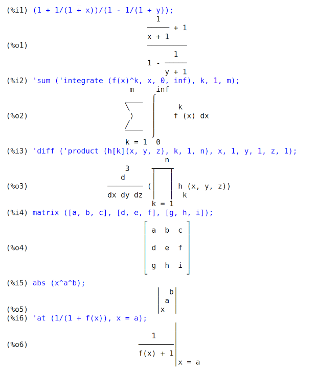
Same expressions, displayed using only ASCII characters
(display2d_unicode equal to false),
shown as an image:
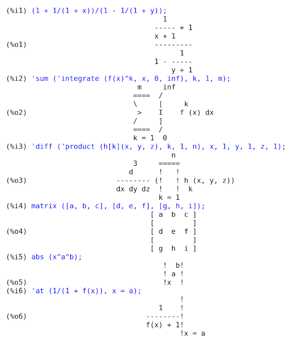
Footnotes:
[1] https://en.wikipedia.org/wiki/Box-drawing_character
display_format_internal — Variable
Default value: false
When display_format_internal is true, expressions are displayed
without being transformed in ways that hide the internal mathematical
representation. The display then corresponds to what inpart returns
rather than part.
Examples:
User part inpart
a-b; a - b a + (- 1) b
a - 1
a/b; - a b
b
1/2
sqrt(x); sqrt(x) x
4 X 4
X*4/3; --- - X
3 3
See also: inpart, part.
display_index_separator — Variable
When a symbol A has index display properties declared via declare_index_properties,
the value of the property display_index_separator
is the string or other expression which is displayed between indices.
The value of display_index_separator
is assigned by put(A, S, display_index_separator),
where S is a string or other expression.
The assigned value is retrieved by get(A, display_index_separator).
The display index separator S can be a string, including an empty string,
or false, indicating the default separator, or any expression.
If not a string and not false, the property value is coerced to a string via string.
If no display index separator is assigned, the default separator is used. The default separator is a comma. There is no way to change the default separator.
Each symbol has its own value of display_index_separator.
See also put, get, and declare_005findex_005fproperties.
Examples:
When a symbol A has index display properties,
the value of the property display_index_separator
is the string or other expression which is displayed between indices.
The value is assigned by put(A, S, display_index_separator),
maxima
(%i1) declare_index_properties (A, [postsuperscript, postsuperscript,
presubscript, presubscript]);
(%o1) done
(%i2) put (A, ";", display_index_separator);
(%o2) ;
(%i3) A[w, x, y, z];
w;x
(%o3) A
y;z
The assigned value is retrieved by get(A, display_index_separator).
maxima
(%i1) declare_index_properties (A, [postsuperscript, postsuperscript,
presubscript, presubscript]);
(%o1) done
(%i2) put (A, ";", display_index_separator);
(%o2) ;
(%i3) get (A, display_index_separator);
(%o3) ;
The display index separator S can be a string, including an empty string,
or false, indicating the default separator, or any expression.
maxima
(%i1) declare_index_properties (A, [postsuperscript, postsuperscript,
presubscript, presubscript]);
(%o1) done
(%i2) A[w, x, y, z];
w, x
(%o2) A
y, z
(%i3) put (A, "-", display_index_separator);
(%o3) -
(%i4) A[w, x, y, z];
w-x
(%o4) A
y-z
(%i5) put (A, " ", display_index_separator);
(%o5)
(%i6) A[w, x, y, z];
w x
(%o6) A
y z
(%i7) put (A, "", display_index_separator);
(%o7)
(%i8) A[w, x, y, z];
wx
(%o8) A
yz
(%i9) put (A, false, display_index_separator);
(%o9) false
(%i10) A[w, x, y, z];
w, x
(%o10) A
y, z
(%i11) put (A, 'foo, display_index_separator);
(%o11) foo
(%i12) A[w, x, y, z];
wfoox
(%o12) A
yfooz
If no display index separator is assigned, the default separator is used. The default separator is a comma.
maxima
(%i1) declare_index_properties (A, [postsuperscript, postsuperscript,
presubscript, presubscript]);
(%o1) done
(%i2) A[w, x, y, z];
w, x
(%o2) A
y, z
Each symbol has its own value of display_index_separator.
maxima
(%i1) declare_index_properties (A, [postsuperscript, postsuperscript,
presubscript, presubscript]);
(%o1) done
(%i2) put (A, " ", display_index_separator);
(%o2)
(%i3) declare_index_properties (B, [presuperscript, presuperscript,
postsubscript, postsubscript]);
(%o3) done
(%i4) put (B, ";", display_index_separator);
(%o4) ;
(%i5) A[w, x, y, z] + B[w, x, y, z];
w;x w x
(%o5) B + A
y;z y z
See also: put, get, declare_index_properties.
dispterms (expr) — Function
Displays expr in parts one below the other. That is, first the operator
of expr is displayed, then each term in a sum, or factor in a product, or
part of a more general expression is displayed separately. This is useful if
expr is too large to be otherwise displayed. For example if P1,
P2, … are very large expressions then the display program may run
out of storage space in trying to display P1 + P2 + ... all at once.
However, dispterms (P1 + P2 + ...) displays P1, then below it
P2, etc. When not using dispterms, if an exponential expression
is too wide to be displayed as A^B it appears as expt (A, B) (or
as ncexpt (A, B) in the case of A^^B).
Example:
maxima
(%i1) dispterms(2*a*sin(x)+%e^x);
+
2 a sin(x)
x
%e
(%o1) done
expt (a, b) — Function
If an exponential expression is too wide to be displayed as
a^b it appears as expt (a, b) (or as
ncexpt (a, b) in the case of a^^b).
expt and ncexpt are not recognized in input.
exptdispflag — Variable
Default value: true
When exptdispflag is true, Maxima displays expressions
with negative exponents using quotients. See also _0025edispflag.
Example:
maxima
(%i1) exptdispflag:true;
(%o1) true
(%i2) 10^-x;
1
(%o2) ---
x
10
(%i3) exptdispflag:false;
(%o3) false
(%i4) 10^-x;
- x
(%o4) 10
See also: %edispflag.
get_index_properties (a) — Function
Returns the properties for a established by declare_index_properties.
See also remove_005findex_005fproperties.
See also: remove_index_properties.
grind (expr) — Function
The function grind prints expr to the console in a form suitable
for input to Maxima. grind always returns done.
When expr is the name of a function or macro, grind prints the
function or macro definition instead of just the name.
See also string, which returns a string instead of printing its
output. grind attempts to print the expression in a manner which makes
it slightly easier to read than the output of string.
grind evaluates its argument.
Examples:
maxima
(%i1) aa + 1729;
(%o1) aa + 1729
(%i2) grind (%);
aa+1729$
(%o2) done
(%i3) [aa, 1729, aa + 1729];
(%o3) [aa, 1729, aa + 1729]
(%i4) grind (%);
[aa,1729,aa+1729]$
(%o4) done
(%i5) matrix ([aa, 17], [29, bb]);
[ aa 17 ]
(%o5) [ ]
[ 29 bb ]
(%i6) grind (%);
matrix([aa,17],[29,bb])$
(%o6) done
(%i7) set (aa, 17, 29, bb);
(%o7) {17, 29, aa, bb}
(%i8) grind (%);
{17,29,aa,bb}$
(%o8) done
(%i9) exp (aa / (bb + 17)^29);
aa
-----------
29
(bb + 17)
(%o9) %e
(%i10) grind (%);
%e^(aa/(bb+17)^29)$
(%o10) done
(%i11) expr: expand ((aa + bb)^10);
10 9 2 8 3 7 4 6
(%o11) bb + 10 aa bb + 45 aa bb + 120 aa bb + 210 aa bb
5 5 6 4 7 3 8 2
+ 252 aa bb + 210 aa bb + 120 aa bb + 45 aa bb
9 10
+ 10 aa bb + aa
(%i12) grind (expr);
bb^10+10*aa*bb^9+45*aa^2*bb^8+120*aa^3*bb^7+210*aa^4*bb^6
+252*aa^5*bb^5+210*aa^6*bb^4+120*aa^7*bb^3+45*aa^8*bb^2
+10*aa^9*bb+aa^10$
(%o12) done
(%i13) string (expr);
(%o13) bb^10+10*aa*bb^9+45*aa^2*bb^8+120*aa^3*bb^7+210*aa^4*bb^6\
+252*aa^5*bb^5+210*aa^6*bb^4+120*aa^7*bb^3+45*aa^8*bb^2+10*aa^9*\
bb+aa^10
(%i14) cholesky (A):= block ([n : length (A), L : copymatrix (A),
p : makelist (0, i, 1, length (A))],
for i thru n do for j : i thru n do
(x : L[i, j], x : x - sum (L[j, k] * L[i, k], k, 1, i - 1),
if i = j then p[i] : 1 / sqrt(x) else L[j, i] : x * p[i]),
for i thru n do L[i, i] : 1 / p[i],
for i thru n do for j : i + 1 thru n do L[i, j] : 0, L)$
define: warning: redefining the built-in operator cholesky
(%i15) grind (cholesky);
cholesky(A):=block(
[n:length(A),L:copymatrix(A),
p:makelist(0,i,1,length(A))],
for i thru n do
(for j from i thru n do
(x:L[i,j],x:x-sum(L[j,k]*L[i,k],k,1,i-1),
if i = j then p[i]:1/sqrt(x)
else L[j,i]:x*p[i])),
for i thru n do L[i,i]:1/p[i],
for i thru n do (for j from i+1 thru n do L[i,j]:0),L)$
(%o15) done
(%i16) string (fundef (cholesky));
(%o16) cholesky(A):=block([n:length(A),L:copymatrix(A),p:makelis\
t(0,i,1,length(A))],for i thru n do (for j from i thru n do (x:L\
[i,j],x:x-sum(L[j,k]*L[i,k],k,1,i-1),if i = j then p[i]:1/sqrt(x\
) else L[j,i]:x*p[i])),for i thru n do L[i,i]:1/p[i],for i thru \
n do (for j from i+1 thru n do L[i,j]:0),L)
See also: string.
ibase — Variable
Default value: 10
ibase is the base for integers read by Maxima.
ibase may be assigned any integer between 2 and 36 (decimal), inclusive.
When ibase is greater than 10,
the numerals comprise the decimal numerals 0 through 9
plus letters of the alphabet A, B, C, …,
as needed to make ibase digits in all.
Letters are interpreted as digits only if the first digit is 0 through 9.
Uppercase and lowercase letters are not distinguished.
The numerals for base 36, the largest acceptable base,
comprise 0 through 9 and A through Z.
Whatever the value of ibase,
when an integer is terminated by a decimal point,
it is interpreted in base 10.
See also obase.
Examples:
ibase less than 10 (for example binary numbers).
maxima
(%i1) ibase : 2 $
(%i2) obase;
(%o2) 10
(%i3) 1111111111111111;
(%o3) 65535
ibase greater than 10.
Letters are interpreted as digits only if the first digit is 0
through 9 which means that hexadecimal numbers might need to
be prepended by a 0.
maxima
(%i1) ibase : 16 $
(%i2) obase;
(%o2) 10
(%i3) 1000;
(%o3) 4096
(%i4) abcd;
(%o4) abcd
(%i5) symbolp (abcd);
(%o5) true
(%i6) 0abcd;
(%o6) 43981
(%i7) symbolp (0abcd);
(%o7) false
When an integer is terminated by a decimal point, it is interpreted in base 10.
maxima
(%i1) ibase : 36 $
(%i2) obase;
(%o2) 10
(%i3) 1234;
(%o3) 49360
(%i4) 1234.;
(%o4) 1234
See also: obase.
ldisp (expr_1, …, expr_n) — Function
Displays expressions expr_1, …, expr_n to the console as
printed output. ldisp assigns an intermediate expression label to each
argument and returns the list of labels.
See also disp, display, and ldisplay.
Examples:
maxima
(%i1) e: (a+b)^3;
3
(%o1) (b + a)
(%i2) f: expand (e);
3 2 2 3
(%o2) b + 3 a b + 3 a b + a
(%i3) ldisp (e, f);
3
(%t3) (b + a)
3 2 2 3
(%t4) b + 3 a b + 3 a b + a
(%o4) [%t3, %t4]
(%i5) %t3;
3
(%o5) (b + a)
(%i6) %t4;
3 2 2 3
(%o6) b + 3 a b + 3 a b + a
See also: disp, display, ldisplay.
ldisplay (expr_1, …, expr_n) — Function
Displays expressions expr_1, …, expr_n to the console as
printed output. Each expression is printed as an equation of the form
lhs = rhs in which lhs is one of the arguments of ldisplay
and rhs is its value. Typically each argument is a variable.
ldisp assigns an intermediate expression label to each equation and
returns the list of labels.
See also display, disp, and ldisp.
Examples:
maxima
(%i1) e: (a+b)^3;
3
(%o1) (b + a)
(%i2) f: expand (e);
3 2 2 3
(%o2) b + 3 a b + 3 a b + a
(%i3) ldisplay (e, f);
3
(%t3) e = (b + a)
3 2 2 3
(%t4) f = b + 3 a b + 3 a b + a
(%o4) [%t3, %t4]
(%i5) %t3;
3
(%o5) e = (b + a)
(%i6) %t4;
3 2 2 3
(%o6) f = b + 3 a b + 3 a b + a
See also: ldisp, display, disp.
leftjust — Variable
Default value: false
When leftjust is true, equations in 2D-display are drawn left
justified rather than centered.
See also display2d to switch between 1D- and 2D-display.
Example:
maxima
(%i1) expand((x+1)^3);
3 2
(%o1) x + 3 x + 3 x + 1
(%i2) leftjust:true$
(%i3) expand((x+1)^3);
3 2
(%o3) x + 3 x + 3 x + 1
See also: display2d.
linel — Variable
Default value: 79
linel is the assumed width (in characters) of the console display for the
purpose of displaying expressions. linel may be assigned any value by
the user, although very small or very large values may be impractical. Text
printed by built-in Maxima functions, such as error messages and the output of
describe, is not affected by linel.
See also: describe.
lispdisp — Variable
Default value: false
When lispdisp is true, Lisp symbols are displayed with a leading
question mark ?. Otherwise, Lisp symbols are displayed with no leading
mark. This has the same effect for 1-d and 2-d display.
Examples:
maxima
(%i1) lispdisp: false$
(%i2) ?foo + ?bar;
(%o2) foo + bar
(%i3) lispdisp: true$
(%i4) ?foo + ?bar;
(%o4) ?foo + ?bar
negsumdispflag — Variable
Default value: true
When negsumdispflag is true, x - y displays as x - y
instead of as - y + x. Setting it to false causes the special
check in display for the difference of two expressions to not be done. One
application is that thus a + %i*b and a - %i*b may both be
displayed the same way.
obase — Variable
Default value: 10
obase is the base for integers displayed by Maxima.
obase may be assigned any integer between 2 and 36 (decimal), inclusive.
When obase is greater than 10,
the numerals comprise the decimal numerals 0 through 9
plus capital letters of the alphabet A, B, C, …, as needed.
A leading 0 digit is displayed if the leading digit is otherwise a letter.
The numerals for base 36, the largest acceptable base,
comprise 0 through 9, and A through Z.
See also ibase.
Examples:
maxima
(%i1) obase : 2;
(%o1) 10
(%i2) 2^8 - 1;
(%o2) 11111111
(%i3) obase : 8;
(%o3) 10
(%i4) 8^8 - 1;
(%o4) 77777777
(%i5) obase : 16;
(%o5) 10
(%i6) 16^8 - 1;
(%o6) 0FFFFFFFF
(%i7) obase : 36;
(%o7) 10
(%i8) 36^8 - 1;
(%o8) 0ZZZZZZZZ
See also: ibase.
pfeformat — Variable
Default value: false
When pfeformat is true, a ratio of integers is displayed with the
solidus (forward slash) character, and an integer denominator n is
displayed as a leading multiplicative term 1/n.
Examples:
maxima
(%i1) pfeformat: false$
(%i2) 2^16/7^3;
65536
(%o2) -----
343
(%i3) (a+b)/8;
b + a
(%o3) -----
8
(%i4) pfeformat: true$
(%i5) 2^16/7^3;
(%o5) 65536/343
(%i6) (a+b)/8;
(%o6) (1/8) (b + a)
powerdisp — Variable
Default value: false
When powerdisp is true,
a sum is displayed with its terms in order of increasing power.
Thus a polynomial is displayed as a truncated power series,
with the constant term first and the highest power last.
By default, terms of a sum are displayed in order of decreasing power.
Example:
maxima
(%i1) powerdisp:true;
(%o1) true
(%i2) x^2+x^3+x^4;
2 3 4
(%o2) x + x + x
(%i3) powerdisp:false;
(%o3) false
(%i4) x^2+x^3+x^4;
4 3 2
(%o4) x + x + x
print (expr_1, …, expr_n) — Function
Evaluates and displays expr_1, …, expr_n one after another, from left to right, starting at the left edge of the console display.
The value returned by print is the value of its last argument.
print does not generate intermediate expression labels.
See also display, disp, ldisplay, and
ldisp. Those functions display one expression per line, while
print attempts to display two or more expressions per line.
To display the contents of a file, see printfile.
Examples:
maxima
(%i1) r: print ("(a+b)^3 is", expand ((a+b)^3), "log (a^10/b) is", radcan (log (a^10/b)))$
3 2 2 3
(a+b)^3 is b + 3 a b + 3 a b + a log (a^10/b) is
10 log(a) - log(b)
(%i2) r;
(%o2) 10 log(a) - log(b)
(%i3) disp ("(a+b)^3 is", expand ((a+b)^3), "log (a^10/b) is", radcan (log (a^10/b)))$
(a+b)^3 is
3 2 2 3
b + 3 a b + 3 a b + a
log (a^10/b) is
10 log(a) - log(b)
See also: display, disp, ldisplay, ldisp, printfile.
remove_index_properties (a, b, c, …) — Function
Removes the properties established by declare_index_properties.
All index properties are removed from each symbol a, b, c, ….
remove_index_properties quotes (does not evaluate) its arguments.
sqrtdispflag — Variable
Default value: true
When sqrtdispflag is false, causes sqrt to display with
exponent 1/2.
stardisp — Variable
Default value: false
When stardisp is true, multiplication is
displayed with an asterisk * between operands.
ttyoff — Variable
Default value: false
When ttyoff is true, output expressions are not displayed.
Output expressions are still computed and assigned labels. See labels.
Text printed by built-in Maxima functions, such as error messages and the output
of describe, is not affected by ttyoff.
See also: labels, describe.
with_default_2d_display (expr) — Function
While maxima by default realizes 2d Output using ASCII-Art some frontend
change that to TeX, MathML or a specific XML dialect that better suits
the needs for this specific frontend. with_default_2d_display
temporarily switches maxima to the default 2D ASCII Art formatter for
outputting the result of expr.
See also set_alt_display and display2d.
See also: set_alt_display, display2d.
Data Types and Structures
concat (arg_1, arg_2, …) — Function
Concatenates its arguments. The arguments must evaluate to atoms. The return value is a symbol if the first argument is a symbol and a string otherwise.
concat evaluates its arguments. The single quote ' prevents
evaluation.
See also sconcat, that works on non-atoms, too, simplode,
string and eval_005fstring.
For complex string conversions see also printf.
(%i1) y: 7$
(%i2) z: 88$
(%i3) concat (y, z/2);
(%o3) 744
(%i4) concat ('y, z/2);
(%o4) y44
A symbol constructed by concat may be assigned a value and appear in
expressions. The :: (double colon) assignment operator evaluates its
left-hand side.
(%i5) a: concat ('y, z/2);
(%o5) y44
(%i6) a:: 123;
(%o6) 123
(%i7) y44;
(%o7) 123
(%i8) b^a;
y44
(%o8) b
(%i9) %, numer;
123
(%o9) b
Note that although concat (1, 2) looks like a number, it is a string.
(%i10) concat (1, 2) + 3;
(%o10) 12 + 3
See also: sconcat, simplode, string, eval_string, printf, ::.
sconcat (arg_1, arg_2, …) — Function
Concatenates its arguments into a string. Unlike concat, the
arguments do not need to be atoms.
See also concat, simplode, string and eval_005fstring.
For complex string conversions see also printf.
(%i1) sconcat ("xx[", 3, "]:", expand ((x+y)^3));
(%o1) xx[3]:y^3+3*x*y^2+3*x^2*y+x^3
Another purpose for sconcat is to convert arbitrary objects to strings.
(%i1) sconcat (x);
(%o1) x
(%i2) stringp(%);
(%o2) true
See also: concat, simplode, string, eval_string, printf.
string (expr) — Function
Converts expr to Maxima’s linear notation just as if it had been typed
in.
The return value of string is a string, and thus it cannot be used in a
computation.
See also concat, sconcat, simplode and
eval_005fstring.
See also: concat, sconcat, simplode, eval_string.
stringdisp — Variable
Default value: false
When stringdisp is true, strings are displayed enclosed in double
quote marks. Otherwise, quote marks are not displayed.
stringdisp is always true when displaying a function definition.
Examples:
(%i1) stringdisp: false$
(%i2) "This is an example string.";
(%o2) This is an example string.
(%i3) foo () :=
print ("This is a string in a function definition.");
(%o3) foo() :=
print("This is a string in a function definition.")
(%i4) stringdisp: true$
(%i5) "This is an example string.";
(%o5) "This is an example string."
File Input and Output
appendfile (filename) — Function
Appends a console transcript to filename. appendfile is the same
as writefile, except that the transcript file, if it exists, is
always appended.
closefile closes the transcript file opened by appendfile or
writefile.
See also: writefile, closefile.
batch (filename) — Function
batch(filename) reads Maxima expressions from filename and
evaluates them. batch searches for filename in the list
file_005fsearch_005fmaxima. See also file_005fsearch.
batch(S) reads Maxima expressions from the input stream S
as created by openr.
The behavior of batch in this case is the same as if the input
were a file name, and in the remainder of this description,
what is said about input files applies to input streams as well,
except that the comments about searching for files do not apply to streams.
batch(filename, demo) is like demo(filename).
In this case batch searches for filename in the list
file_005fsearch_005fdemo. See demo.
batch(filename, test) is like run_testsuite with the
option display_all=true. For this case batch searches
filename in the list file_search_maxima and not in the list
file_search_tests like run_testsuite. Furthermore,
run_testsuite runs tests which are in the list
testsuite_005ffiles. With batch it is possible to run any file in
a test mode, which can be found in the list file_search_maxima. This is
useful, when writing a test file.
filename comprises a sequence of Maxima expressions, each terminated with
; or $. The special variable % and the function
%th refer to previous results within the file. The file may include
:lisp constructs. Spaces, tabs, and newlines in the file are ignored.
A suitable input file may be created by a text editor or by the
stringout function.
batch reads each input expression from filename, displays
the input to the console, computes the corresponding output expression,
and displays the output expression. Input labels are assigned to the
input expressions and output labels are assigned to the output
expressions. batch evaluates every input expression in the file
unless there is an error. If user input is requested (by asksign
or askinteger, for example) batch pauses to collect
the requisite input and then continue; if batch_answers_from_file
is true, the input is read from the file itself. See also
batch_005fanswers_005ffrom_005ffile.
It may be possible to halt batch by typing control-C at the
console. The effect of control-C depends on the underlying Lisp
implementation.
batch has several uses, such as to provide a reservoir for working
command lines, to give error-free demonstrations, or to help organize one’s
thinking in solving complex problems.
batch evaluates its arguments.
When called with no second argument or with the option demo,
batch returns the path of filename,
if the argument is a file name,
or the path of the file for which the input stream was opened,
if the argument is a file input stream.
If the argument is a string input stream,
a representation of the input stream is returned.
When called with the option test, the return value
is a an empty list [] or a list with filename and the numbers of
the tests which have failed.
See also load, batchload,
batch_answers_from_file, and demo.
See also: file_search_maxima, file_search, openr, file_search_demo, demo, run_testsuite, file_search_tests, testsuite_files, %, %th, stringout, asksign, askinteger, batch_answers_from_file, load, batchload.
batch_answers_from_file — Variable
Default value: false
If true, then batch reads answers to interactive questions
from its input file or stream.
Example: Maxima’s interactive testsuite includes something like following.
maxima
[asksign (foo), sign (foo), sign (foo)];
p;
[pos, pos, pos];
The first line makes Maxima ask a question; when
batch_answers_from_file is true, the second line is read
as the answer to the question; and the third line provides the expected
result.
The command-line option --batch-string binds
batch_answers_from_file to true. The run_testsuite
function, as a default, also binds batch_answers_from_file to
true. See also command_line_options and run_005ftestsuite.
See also: command_line_options, run_testsuite.
batchload (filename) — Function
Reads Maxima expressions from input file filename or input stream S
and evaluates them,
without displaying the input or output expressions and without assigning labels to
output expressions. Printed output (such as produced by print or
describe) is displayed, however.
The special variable % and the function %th refer to previous
results from the interactive interpreter, not results within the file.
The file cannot include :lisp constructs.
batchload evaluates its argument.
batchload returns the path of filename,
if the argument is a file name,
or the path of the file for which the input stream was opened,
if the argument is a file input stream.
If the argument is a string input stream,
a representation of the input stream is returned.
See also batch, and load.
See also: print, describe, %, %th, batch, load.
closefile () — Function
Closes the transcript file opened by writefile or appendfile.
See also: writefile, appendfile.
directory (path) — Function
Returns a list of the files and directories found in path in the file system.
path may contain wildcard characters (i.e., characters which represent unspecified parts of the path), which include at least the asterisk on most systems, and possibly other characters, depending on the system.
directory relies on the Lisp function DIRECTORY,
which may have implementation-specific behavior.
file_output_append — Variable
Default value: false
file_output_append governs whether file output functions append or
truncate their output file. When file_output_append is true, such
functions append to their output file. Otherwise, the output file is truncated.
save, stringout, and with_stdout respect
file_output_append. Other functions which write output files do not
respect file_output_append. In particular, plotting and translation
functions always truncate their output file, and tex and
appendfile always append.
See also: save, stringout, with_stdout, tex, appendfile.
file_search (filename) — Function
file_search searches for the file filename and returns the path to
the file (as a string) if it can be found; otherwise file_search returns
false. file_search (filename) searches in the default
search directories, which are specified by the
file_search_maxima, file_search_lisp, and
file_search_demo variables.
file_search first checks if the actual name passed exists,
before attempting to match it to “wildcard” file search patterns.
See file_search_maxima concerning file search patterns.
The argument filename can be a path and file name, or just a file name, or, if a file search directory includes a file search pattern, just the base of the file name (without an extension). For example,
maxima
file_search ("/home/wfs/special/zeta.mac");
file_search ("zeta.mac");
file_search ("zeta");
all find the same file, assuming the file exists and
/home/wfs/special/###.mac is in file_search_maxima.
file_search (filename, pathlist) searches only in the
directories specified by pathlist, which is a list of strings. The
argument pathlist supersedes the default search directories, so if the
path list is given, file_search searches only the ones specified, and not
any of the default search directories. Even if there is only one directory in
pathlist, it must still be given as an one-element list.
The user may modify the default search directories.
See file_005fsearch_005fmaxima.
file_search is invoked by load with file_search_maxima and
file_search_lisp as the search directories.
See also file_005fsearch_005fcache.
See also: file_search_maxima, file_search_lisp, file_search_demo, load, file_search_cache.
file_search_cache — Variable
Default value: auto
file_search_cache controls the use of a cache by file_search in
order to speed up the search. Currently, it can only speed up searches where
the filename part does not contain wildcards (but the directory part may).
When file_search_cache is auto (the default value), the cache
will be activated if a one-time check determines that the system (Lisp
implementation, file system) fulfills the requirements. This can be overridden
by setting file_search_cache to true, which is not recommended.
The value false prevents the use of the cache.
See also file_005fsearch.
See also: file_search.
file_search_maxima — Variable
These variables specify lists of directories to be searched by
load, demo, and some other Maxima functions. The default
values of these variables name various directories in the Maxima installation.
The user can modify these variables, either to replace the default values or to append additional directories. For example,
maxima
file_search_maxima: ["/usr/local/foo/*.mac",
"/usr/local/bar/*.mac"]$
replaces the default value of file_search_maxima, while
maxima
file_search_maxima: append (file_search_maxima,
["/usr/local/foo/*.mac", "/usr/local/bar/*.mac"])$
appends two additional directories. It may be convenient to put such an
expression in the file maxima-init.mac so that the file search path is
assigned automatically when Maxima starts.
See also Introduction-for-Runtime-Environment.
Each element of the search list is a Common Lisp wildcard pathname.
Briefly, a wildcard filename looks like "*.lisp", which matches
any filename with an extension of "lisp". A directory
component of * matches any directory in the current directory,
and ** matches any directory and subdirectories in the current
directory.
So, file_search_maxima includes
"/home/username/.maxima/**/*.mac". This means look in all
subdirectories of "/home/username/.maxima/" for files with
extension "mac". This includes subdirectories of
subdirectories. Thus, load("file") will find
"/home/username/.maxima/dir1/subdir1/file.mac".
To only search for a single level of subdirectories, use
"/home/username/.maxima/*/*.mac". This means Maxima will not
find the file "/home/username/.maxima/dir1/subdir1/file.mac"
when Maxima tries to, say, load("file").
Further information about Common Lisp pathnames maybe be found in http://www.lispworks.com/documentation/HyperSpec/Body/19_b.htmCLHS Section 19.2: Pathnames.
See also: load, demo, Introduction-for-Runtime-Environment.
file_type (filename) — Function
Returns a guess about the content of filename, based on the filename extension. filename need not refer to an actual file; no attempt is made to open the file and inspect the content.
The return value is a symbol, either object, lisp, or
maxima. If the extension is matches one of the values in
file_type_maxima, file_type returns maxima. If the
extension matches one of the values in file_type_lisp, file_type
returns lisp. If none of the above, file_type returns
object.
See also pathname_005ftype.
See file_type_maxima and file_type_lisp for the default values.
Examples:
maxima
(%i1) map('file_type,
["test.lisp", "test.mac", "test.dem", "test.txt"]);
(%o1) [lisp, maxima, maxima, object]
See also: pathname_type, file_type_maxima, file_type_lisp.
file_type_lisp — Variable
Default value: [l, lsp, lisp]
file_type_lisp is a list of file extensions that maxima recognizes
as denoting a Lisp source file.
See also file_005ftype.
See also: file_type.
file_type_maxima — Variable
Default value: [mac, mc, demo, dem, dm1, dm2, dm3, dmt, wxm]
file_type_maxima is a list of file extensions that maxima recognizes
as denoting a Maxima source file.
See also file_005ftype.
See also: file_type.
filename_merge (path, filename) — Function
Constructs a modified path from path and filename. If the final
component of path is of the form ###.something, the component
is replaced with filename.something. Otherwise, the final
component is simply replaced by filename.
The result is a Lisp pathname object.
fortindent — Variable
Default value: 0
fortindent controls the left margin indentation of
expressions printed out by the fortran command. 0 gives normal
printout (i.e., 6 spaces), and positive values will causes the
expressions to be printed farther to the right.
See also: fortran.
fortran (expr) — Function
Prints expr as a Fortran statement.
The output line is indented with spaces.
If the line is too long, fortran prints continuation lines.
fortran prints the exponentiation operator ^ as **,
and prints a complex number a + b %i in the form (a,b).
expr may be an equation. If so, fortran prints an assignment
statement, assigning the right-hand side of the equation to the left-hand side.
In particular, if the right-hand side of expr is the name of a matrix,
then fortran prints an assignment statement for each element of the
matrix.
If expr is not something recognized by fortran,
the expression is printed in grind format without complaint.
fortran does not know about lists, arrays, or functions.
fortindent controls the left margin of the printed lines.
0 is the normal margin (i.e., indented 6 spaces). Increasing
fortindent causes expressions to be printed further to the right.
When fortspaces is true, fortran fills out
each printed line with spaces to 80 columns.
fortran evaluates its arguments; quoting an argument defeats evaluation.
fortran always returns done.
See also the function function_005ff90 for printing one or more
expressions as a Fortran 90 program.
Examples:
maxima
(%i1) expr: (a + b)^12$
(%i2) fortran (expr);
(b+a)**12
(%o2) done
(%i3) fortran ('x=expr);
x = (b+a)**12
(%o3) done
(%i4) fortran ('x=expand (expr));
x = b**12+12*a*b**11+66*a**2*b**10+220*a**3*b**9+495*a**4*b**8+792
1 *a**5*b**7+924*a**6*b**6+792*a**7*b**5+495*a**8*b**4+220*a**9*b
2 **3+66*a**10*b**2+12*a**11*b+a**12
(%o4) done
(%i5) fortran ('x=7+5*%i);
x = (7,5)
(%o5) done
(%i6) fortran ('x=[1,2,3,4]);
x(1) = 1
x(2) = 2
x(3) = 3
x(4) = 4
(%o6) done
(%i7) f(x) := x^2$
(%i8) fortran (f);
f
(%o8) done
See also: grind, fortindent, fortspaces, function_f90.
fortspaces — Variable
Default value: false
When fortspaces is true, fortran fills out
each printed line with spaces to 80 columns.
get_tex_environment (op) — Function
Customize the TeX environment output by tex.
As maintained by these functions, the TeX environment comprises two strings:
one is printed before any other TeX output, and the other is printed after.
Only the TeX environment of the top-level operator in an expression is output; TeX environments associated with other operators are ignored.
get_tex_environment returns the TeX environment which is applied
to the operator op; returns the default if no other environment
has been assigned.
set_tex_environment assigns the TeX environment for the operator
op.
Examples:
maxima
(%i1) get_tex_environment (":=");
(%o1) [
\begin{verbatim}
, ;
\end{verbatim}
]
(%i2) tex (f (x) := 1 - x);
\begin{verbatim}
f(x):=1-x;
\end{verbatim}
(%o2) false
(%i3) set_tex_environment (":=", "$$", "$$");
(%o3) [$$, $$]
(%i4) tex (f (x) := 1 - x);
$$f(x):=1-x$$
(%o4) false
get_tex_environment_default () — Function
Customize the TeX environment output by tex.
As maintained by these functions, the TeX environment comprises two strings:
one is printed before any other TeX output, and the other is printed after.
get_tex_environment_default returns the TeX environment which is
applied to expressions for which the top-level operator has no
specific TeX environment (as assigned by set_tex_environment).
set_tex_environment_default assigns the default TeX environment.
Examples:
maxima
(%i1) get_tex_environment_default ();
(%o1) [$$, $$]
(%i2) tex (f(x) + g(x));
$$g\left(x\right)+f\left(x\right)$$
(%o2) false
(%i3) set_tex_environment_default ("\\begin{equation}
(%o3) [\begin{equation}
,
\end{equation}]
(%i4) ", "
\begin{equation}
g\left(x\right)+f\left(x\right)
\end{equation}
(%o4) false
(%i5) \\end{equation}");
load (filename) — Function
Evaluates expressions in filename, thus bringing variables, functions, and other objects into Maxima. The binding of any existing object is clobbered by the binding recovered from filename.
filename must be a string, symbol,
or Lisp pathname (as created by filename_merge).
To find the file, load calls
file_search with file_search_maxima and
file_search_lisp as the search directories. If load succeeds, it
returns the name of the file. Otherwise load prints an error message.
load works equally well for Lisp code and Maxima code. Files created by
save, translate_file, and compile_file, which
create Lisp code, and stringout, which creates Maxima code, can all
be processed by load. load calls loadfile to load Lisp
files and batchload to load Maxima files.
load does not recognize :lisp constructs in Maxima files, and
while processing filename, the global variables _, __,
%, and %th have whatever bindings they had when load was
called.
Note also that structures will only be read back as structures if
they have been defined by defstruct before the load command
is called.
See also loadfile, for Lisp files; and batch, batchload, and
demo. for Maxima files.
See file_search for more detail about the file search mechanism.
The numericalio chapter describes many functions
for loading csv and other data files.
During Maxima file loading, the variable load_pathname is bound to the pathname of the file
being loaded.
load evaluates its argument.
See also: filename_merge, file_search, file_search_maxima, file_search_lisp, save, translate_file, compile_file, stringout, loadfile, batchload, batch, demo, numericalio, load_pathname.
load_pathname — Variable
Default value: false
When a file is loaded with the functions load, loadfile or
batchload the system variable load_pathname is bound to the
pathname of the file which is processed.
The variable load_pathname can be accessed from the file during the
loading.
Example:
Suppose we have a batchfile test.mac in the directory
"/home/dieter/workspace/mymaxima/temp/" with the following commands
maxima
print("The value of load_pathname is: ", load_pathname)$
print("End of batchfile")$
then we get the following output
maxima
(%i1) load("/home/dieter/workspace/mymaxima/temp/test.mac")$
The value of load_pathname is:
/home/dieter/workspace/mymaxima/temp/test.mac
End of batchfile
See also: load, loadfile, batchload.
loadfile (filename) — Function
Evaluates Lisp expressions in filename. loadfile does not invoke
file_search, so filename must include the file extension and
as much of the path as needed to find the file.
loadfile can process files created by save,
translate_file, and compile_005ffile. The user may find it
more convenient to use load instead of loadfile.
See also: file_search, save, translate_file, compile_file, load.
loadprint — Variable
Default value: true
loadprint tells whether to print a message when a file is loaded.
When loadprint is true, always print a message.
When loadprint is 'loadfile, print a message only if
a file is loaded by the function loadfile.
When loadprint is 'autoload,
print a message only if a file is automatically loaded.
See setup_005fautoload.
When loadprint is false, never print a message.
See also: setup_autoload.
pathname_directory (pathname) — Function
These functions return the components of pathname.
Examples:
maxima
(%i1) pathname_directory("/home/dieter/maxima/changelog.txt");
(%o1) /home/dieter/maxima/
(%i2) pathname_name("/home/dieter/maxima/changelog.txt");
(%o2) changelog
(%i3) pathname_type("/home/dieter/maxima/changelog.txt");
(%o3) txt
printfile (path) — Function
Prints the file named by path to the console. path may be a string or a symbol; if it is a symbol, it is converted to a string.
If path names a file which is accessible from the current working
directory, that file is printed to the console. Otherwise, printfile
attempts to locate the file by appending path to each of the elements of
file_search_usage via filename_005fmerge.
printfile returns path if it names an existing file,
or otherwise the result of a successful filename merge.
See also: file_search_usage, filename_merge.
save (filename, name_1, name_2, name_3, …) — Function
Stores the current values of name_1, name_2, name_3, …,
in filename. The arguments are the names of variables, functions, or
other objects. If a name has no value or function associated with it, it is
ignored. save returns filename.
save stores data in the form of Lisp expressions.
If filename ends in .lisp the
data stored by save may be recovered by load (filename).
See load.
The global flag file_output_append governs whether save appends or
truncates the output file. When file_output_append is true,
save appends to the output file. Otherwise, save truncates the
output file. In either case, save creates the file if it does not yet
exist.
The special form save (filename, values, functions, labels, ...)
stores the items named by values, functions,
labels, etc. The names may be any specified by the variable
infolists. values comprises all user-defined variables.
The special form save (filename, [m, n]) stores the
values of input and output labels m through n. Note that m
and n must be literal integers. Input and output labels may also be
stored one by one, e.g., save ("foo.1", %i42, %o42).
save (filename, labels) stores all input and output labels.
When the stored labels are recovered, they clobber existing labels.
The special form save (filename, name_1=expr_1, name_2=expr_2, ...) stores the values of expr_1,
expr_2, …, with names name_1, name_2, …
It is useful to apply this form to input and output labels, e.g.,
save ("foo.1", aa=%o88). The right-hand side of the equality in this
form may be any expression, which is evaluated. This form does not introduce
the new names into the current Maxima environment, but only stores them in
filename.
These special forms and the general form of save may be mixed at will.
For example, save (filename, aa, bb, cc=42, functions, [11, 17]).
The special form save (filename, all) stores the current state of
Maxima. This includes all user-defined variables, functions, arrays, etc., as
well as some automatically defined items. The saved items include system
variables, such as file_search_maxima or showtime, if they
have been assigned new values by the user; see myoptions.
save evaluates filename and quotes all other arguments.
See also: load, file_output_append, values, functions, labels, infolists, file_search_maxima, showtime, myoptions.
stringout (filename, expr_1, expr_2, expr_3, …) — Function
stringout writes expressions to a file in the same form the expressions
would be typed for input. The file can then be used as input for the
batch or demo commands, and it may be edited for any purpose.
stringout can be executed while writefile is in progress.
The global flag file_output_append governs whether stringout
appends or truncates the output file. When file_output_append is
true, stringout appends to the output file. Otherwise,
stringout truncates the output file. In either case, stringout
creates the file if it does not yet exist.
The general form of stringout writes the values of one or more
expressions to the output file. Note that if an expression is a
variable, only the value of the variable is written and not the name
of the variable. As a useful special case, the expressions may be
input labels (%i1, %i2, %i3, …) or output labels
(%o1, %o2, %o3, …).
If grind is true, stringout formats the output using the
grind format. Otherwise the string format is used. See
grind and string.
The special form stringout (filename, [m, n]) writes
the values of input labels m through n, inclusive.
The special form stringout (filename, input) writes all
input labels to the file.
The special form stringout (filename, functions) writes all
user-defined functions (named by the global list functions) to the
file.
The special form stringout (filename, values) writes all
user-assigned variables (named by the global list values) to the file.
Each variable is printed as an assignment statement, with the name of the
variable, a colon, and its value. Note that the general form of
stringout does not print variables as assignment statements.
See also: batch, demo, writefile, file_output_append, grind, functions, values.
tex (expr) — Function
Prints a representation of an expression suitable for the TeX document preparation system. The result is a fragment of a document, which can be copied into a larger document but not processed by itself.
tex (expr) prints a TeX representation of expr on the
console.
tex (label) prints a TeX representation of the expression named by
label and assigns it an equation label (to be displayed to the left of the
expression). The TeX equation label is the same as the Maxima label.
destination may be an output stream or file name. When destination
is a file name, tex appends its output to the file. The functions
openw and opena create output streams.
tex (expr, false) and tex (label, false)
return their TeX output as a string.
tex evaluates its first argument after testing it to see if it is a
label. Quote-quote '' forces evaluation of the argument, thereby
defeating the test and preventing the label.
See also tex1 and texput.
Examples:
maxima
(%i1) integrate (1/(1+x^3), x);
2 x - 1
2 atan(-------)
log(x - x + 1) sqrt(3) log(x + 1)
(%o1) - --------------- + ------------- + ----------
6 sqrt(3) 3
(%i2) tex (%o1);
$$-\left({{\log \left(x^2-x+1\right)}\over{6}}\right)+{{\arctan
\left({{2\,x-1}\over{\sqrt{3}}}\right)}\over{\sqrt{3}}}+{{\log
\left(x+1\right)}\over{3}}\leqno{\tt (\%o1)}$$
(%o2) (\%o1)
(%i3) tex (integrate (sin(x), x));
$$-\cos x$$
(%o3) false
(%i4) tex (%o1, "foo.tex");
(%o4) (\%o1)
tex (expr, false) returns its TeX output as a string.
maxima
(%i1) S : tex (x * y * z, false);
(%o1) $$x\,y\,z$$
(%i2) S;
(%o2) $$x\,y\,z$$
See also: tex1, texput.
tex1 (e) — Function
Returns a string which represents the TeX output for the expressions e. The TeX output is not enclosed in delimiters for an equation or any other environment.
See also tex and texput.
Examples:
maxima
(%i1) tex1 (sin(x) + cos(x));
(%o1) \sin x+\cos x
See also: tex, texput.
texput (a, s) — Function
Assign the TeX output for the atom a, which can be a symbol or the name of an operator.
texput (a, s) causes the tex function to interpolate
the string s into the TeX output in place of a.
texput (a, f) causes the tex function to call the
function f to generate TeX output. f must accept one argument,
which is an expression which has operator a,
and must return either a string (the TeX output) or false,
indicating that the TeX function in effect when texput is called
should handle the expression.
f may call tex1 to generate TeX output for the
arguments of the input expression.
texput (a, s, operator_type), where operator_type
is prefix, infix, postfix, nary, or nofix,
causes the tex function to interpolate s into the TeX output in
place of a, and to place the interpolated text in the appropriate
position.
texput (a, [s_1, s_2], matchfix) causes the tex
function to interpolate s_1 and s_2 into the TeX output on either
side of the arguments of a. The arguments (if more than one) are
separated by commas.
texput (a, [s_1, s_2, s_3], matchfix) causes the
tex function to interpolate s_1 and s_2 into the TeX output
on either side of the arguments of a, with s_3 separating the
arguments.
See also tex and tex1.
Examples:
Assign TeX output for a variable.
maxima
(%i1) texput (me,"\\mu_e");
(%o1) \mu_e
(%i2) tex (me);
$$\mu_e$$
(%o2) false
Assign TeX output for an ordinary function (not an operator).
maxima
(%i1) texput (lcm, "\\mathrm{lcm}");
(%o1) \mathrm{lcm}
(%i2) tex (lcm (a, b));
$$\mathrm{lcm}\left(a , b\right)$$
(%o2) false
Call a function to generate TeX output.
maxima
(%i1) texfoo (e) := block ([a, b], [a, b] : args (e),
concat ("\\left[\\stackrel{",tex1(b),"}{",tex1(a),"}\\right]"))$
(%i2) texput (foo, texfoo);
(%o2) texfoo
(%i3) tex (foo (2^x, %pi));
$$\left[\stackrel{\pi}{2^{x}}\right]$$
(%o3) false
Assign TeX output for a prefix operator.
maxima
(%i1) prefix ("grad");
(%o1) grad
(%i2) texput ("grad", " \\nabla ", prefix);
(%o2) \nabla
(%i3) tex (grad f);
$$ \nabla f$$
(%o3) false
Assign TeX output for an infix operator.
maxima
(%i1) infix ("~");
(%o1) ~
(%i2) texput ("~", " \\times ", infix);
(%o2) \times
(%i3) tex (a ~ b);
$$a \times b$$
(%o3) false
Assign TeX output for a postfix operator.
maxima
(%i1) postfix ("##");
(%o1) ##
(%i2) texput ("##", "!!", postfix);
(%o2) !!
(%i3) tex (x ##);
$$x!!$$
(%o3) false
Assign TeX output for a nary operator.
maxima
(%i1) nary ("@@");
(%o1) @@
(%i2) texput ("@@", " \\circ ", nary);
(%o2) \circ
(%i3) tex (a @@ b @@ c @@ d);
$$a \circ b \circ c \circ d$$
(%o3) false
Assign TeX output for a nofix operator.
maxima
(%i1) nofix ("foo");
(%o1) foo
(%i2) texput ("foo", "\\mathsc{foo}", nofix);
(%o2) \mathsc{foo}
(%i3) tex (foo);
$$\mathsc{foo}$$
(%o3) false
Assign TeX output for a matchfix operator.
maxima
(%i1) matchfix ("<<", ">>");
(%o1) <<
(%i2) texput ("<<", [" \\langle ", " \\rangle "], matchfix);
(%o2) [ \langle , \rangle ]
(%i3) tex (<<a>>);
$$ \langle a \rangle $$
(%o3) false
(%i4) tex (<<a, b>>);
$$ \langle a , b \rangle $$
(%o4) false
(%i5) texput ("<<", [" \\langle ", " \\rangle ", " \\, | \\,"],
matchfix);
(%o5) [ \langle , \rangle , \, | \,]
(%i6) tex (<<a>>);
$$ \langle a \rangle $$
(%o6) false
(%i7) tex (<<a, b>>);
$$ \langle a \, | \,b \rangle $$
(%o7) false
See also: tex, tex1.
with_stdout (f, expr_1, expr_2, expr_3, …) — Function
Evaluates expr_1, expr_2, expr_3, … and writes any
output thus generated to a file f or output stream s. The evaluated
expressions are not written to the output. Output may be generated by
print, display, grind, among other functions.
The global flag file_output_append governs whether with_stdout
appends or truncates the output file f. When file_output_append
is true, with_stdout appends to the output file. Otherwise,
with_stdout truncates the output file. In either case,
with_stdout creates the file if it does not yet exist.
with_stdout returns the value of its final argument.
See also writefile and display2d.
(%i1) with_stdout ("tmp.out", for i:5 thru 10 do
print (i, "! yields", i!))$
(%i2) printfile ("tmp.out")$
5 ! yields 120
6 ! yields 720
7 ! yields 5040
8 ! yields 40320
9 ! yields 362880
10 ! yields 3628800
See also: print, display, grind, file_output_append, writefile, display2d.
writefile (filename) — Function
Begins writing a transcript of the Maxima session to filename. All interaction between the user and Maxima is then recorded in this file,
just as it appears on the console.
As the transcript is printed in the console output format, it cannot be reloaded
into Maxima. To make a file containing expressions which can be reloaded,
see save and stringout. save stores expressions in Lisp
form, while stringout stores expressions in Maxima form.
The effect of executing writefile when filename already exists
depends on the underlying Lisp implementation; the transcript file may be
clobbered, or the file may be appended. appendfile always appends to
the transcript file.
It may be convenient to execute playback after writefile to save
the display of previous interactions. As playback displays only the
input and output variables (%i1, %o1, etc.), any output generated
by a print statement in a function (as opposed to a return value) is not
displayed by playback.
closefile closes the transcript file opened by writefile or
appendfile.
See also: save, stringout, appendfile, playback, closefile.
alt-display
alt_display_output_type (form) — Function
Determine the type of output to be printed. Form must be a lisp
form suitable for printing via Maxima’s built-in displa
function. At present, this function returns one of three values:
text, label or unknown.
An example where alt_display_output_type is used. In
my_display, a text form is printed between a pair of tags
TEXT;>> and <<TEXT; while a label form is printed between
a pair tags OUT;>> and <<OUT; in addition to the usual
output label.
The function set_prompt also ensures that input labels are
printed between matching PROMPT;>> and <<PROMPT; tags.
(%i1) (load(“mactex-utilities”), load(“alt-display.mac”)) $
(%i2) define_alt_display(my_display(form),
block([type,txttmplt,labtmplt],
txttmplt:“%TEXT;>>%a%<<TEXT;%”,
labtmplt:“%OUT;>>~%(a) %”,
type:alt_display_output_type(form),
if type=’text then
printf(true,txttmplt,first(form))
else if type=’label then
printf(true,labtmplt,first(form),“$$”,tex1(second(form)),“$$”)
else
block([alt_display1d:false, alt_display2d:false], displa(form)))) $a~a~a%<<OUT;
(%i3) (set_prompt(’prefix, “PROMPT;>>”,’suffix, “<<PROMPT;”), set_alt_display(1,my_display)) $
PROMPT;>>(%i4) <<PROMPT;integrate(x^n,x); PROMPT;>> TEXT;>> Is n equal to -1? <<TEXT; <<PROMPT; n;
OUT;>> (%o4) $$\frac{x^{n+1}}{n+1}$$ <<OUT; PROMPT;>>(%i5) <<PROMPT;
See also: set_prompt.
define_alt_display (function(input), expr) — Function
This function is similar to define: it evaluates its arguments
and expands into a function definition. The function is a
function of a single input input. For convenience, a substitution
is applied to expr after evaluation, to provide easy access to
Lisp variable names.
Set a time-stamp on each prompt:
(%i1) load("alt-display.mac")$
(%i2) display2d: false$
(%i3) define_alt_display(time_stamp(x),
block([alt_display1d:false,alt_display2d:false],
prompt_prefix:printf(false,"~a~%",timedate()),
displa(x)));
(%o3) time_stamp(x):=block(
[\*alt\-display1d\*:false,
\*alt\-display2d\*:false],
\*prompt\-prefix\*
:printf(false,"~a~%",timedate()),displa(x))
(%i4) set_alt_display(1,time_stamp);
(%o4) done
2017-11-27 16:15:58-06:00
(%i5)
The input line %i3 defines time_stamp using
define_alt_display. The output line %o3 shows that the
Maxima variable names alt_display1d, alt_display2d and
prompt_prefix have been replaced by their Lisp translations, as
has displa been replaced by ?displa (the display
function).
The display variables alt_display1d and alt_display2d are
both bound to false in the body of time_stamp to prevent
an infinite recursion in displa.
info_display (form) — Function
This is an alias for the default 1-d display function. It may be used as an alternative 1-d or 2-d display function.
(%i1) load("alt-display.mac")$
(%i2) set_alt_display(2,info_display);
(%o2) done
(%i3) x/y;
(%o3) x/y
mathml_display (form) — Function
Produces MathML output.
(%i1) load("alt-display.mac")$
(%i2) set_alt_display(2,mathml_display);
<math xmlns="http://www.w3.org/1998/Math/MathML"> <mi>mlabel</mi>
<mfenced separators=""><msub><mi>%o</mi> <mn>2</mn></msub>
<mo>,</mo><mi>done</mi> </mfenced> </math>
multi_display_for_texinfo (form) — Function
Produces Texinfo output using all three display functions.
(%i2) set_alt_display(2,multi_display_for_texinfo)$
(%i3) x/(x^2+y^2);
@iftex
@tex
\mbox{\tt\red({\it \%o_3}) \black}$${{x}\over{y^2+x^2}}$$
@end tex
@end iftex
@ifhtml
@html
<math xmlns="http://www.w3.org/1998/Math/MathML"> <mi>mlabel</mi>
<mfenced separators=""><msub><mi>%o</mi> <mn>3</mn></msub>
<mo>,</mo><mfrac><mrow><mi>x</mi> </mrow> <mrow><msup><mrow>
<mi>y</mi> </mrow> <mn>2</mn> </msup> <mo>+</mo> <msup><mrow>
<mi>x</mi> </mrow> <mn>2</mn> </msup> </mrow></mfrac> </mfenced> </math>
@end html
@end ifhtml
@ifinfo
@example
(%o3) x/(y^2+x^2)
@end example
@end ifinfo
reset_displays () — Function
Resets the prompt prefix and suffix to the empty string, and sets both 1-d and 2-d display functions to the default.
set_alt_display (num, display-function) — Function
The input num is the display to set; it may be either 1 or 2. The
second input display-function is the display function to use. The
display function may be either a Maxima function or a lambda
expression.
Here is an example where the display function is a lambda
expression; it just displays the result as TeX.
(%i1) load("alt-display.mac")$
(%i2) set_alt_display(2, lambda([form], tex(?caddr(form))))$
(%i3) integrate(exp(-t^2),t,0,inf);
$${{\sqrt{\pi}}\over{2}}$$
A user-defined display function should take care that it prints its output. A display function that returns a string will appear to display nothing, nor cause any errors.
set_prompt (fix, expr) — Function
Set the prompt prefix or suffix to expr. The input fix must
evaluate to one of prefix, suffix, general,
prolog or epilog. The input expr must evaluate to
either a string or false; if false, the fix is reset
to the default value.
(%i1) load("alt-display.mac")$
(%i2) set_prompt('prefix,printf(false,"It is now: ~a~%",timedate()))$
It is now: 2014-01-07 15:23:23-05:00
(%i3)
The following example shows the effect of each option, except
prolog. Note that the epilog prompt is printed as Maxima
closes down. The general is printed between the end of input and
the output, unless the input line ends in $.
Here is an example to show where the prompt strings are placed.
(%i1) load("alt-display.mac")$
(%i2) set_prompt(prefix, "<<prefix>> ", suffix, "<<suffix>> ",
general, printf(false,"<<general>>~%"),
epilog, printf(false,"<<epilog>>~%"));
(%o2) done
<<prefix>> (%i3) <<suffix>> x/y;
<<general>>
x
(%o3) -
y
<<prefix>> (%i4) <<suffix>> quit();
<<general>>
<<epilog>>
Here is an example that shows how to colorize the input and output when Maxima is running in a terminal or terminal emulator like Emacs
Readers using the info reader in Emacs will
see the actual prompt strings; other readers will see the colorized
output
.
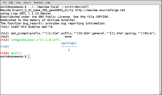
Each prompt string starts with the ASCII escape character (27) followed by an open square bracket (91); each string ends with a lower-case m (109). The webpages https://misc.flogisoft.com/bash/tip_colors_and_formatting and https://www.tldp.org/HOWTO/Bash-Prompt-HOWTO/x329.html provide information on how to use control strings to set the terminal colors.
tex_display (form) — Function
Produces TeX output.
(%i2) set_alt_display(2,tex_display);
\mbox{\tt\red({\it \%o_2}) \black}$$\mathbf{done}$$
(%i3) x/(x^2+y^2);
\mbox{\tt\red({\it \%o_3}) \black}$${{x}\over{y^2+x^2}}$$
engineering-format
engineering_format_floats — Variable
Default value: true
This variable allows to temporarily switch off engineering-format.
(%i1) load("engineering-format");
(%o1) /home/gunter/src/maxima-code/share/contrib/engineering-for\
mat.lisp
(%i2) float(sin(10)/10000);
(%o2) - 54.40211108893698e-6
(%i3) engineering_format_floats:false$
(%i4) float(sin(10)/10000);
(%o4) - 5.440211108893698e-5
See also fpprintprec and float.
See also: fpprintprec, float.
engineering_format_max — Variable
Default value: 0.0
The maximum absolute value that isn’t automatically converted to the engineering format.
See also engineering_format_min and engineering_005fformat_005ffloats.
See also: engineering_format_min, engineering_format_floats.
engineering_format_min — Variable
Default value: 0.0
The minimum absolute value that isn’t automatically converted to the engineering format.
See also engineering_format_max and engineering_005fformat_005ffloats.
(%i1) lst: float([.05,.5,5,500,5000,500000]);
(%o1) [0.05, 0.5, 5.0, 500.0, 5000.0, 500000.0]
(%i2) load("engineering-format");
(%o2) /home/gunter/src/maxima-code/share/contrib/engineering-for\
mat.lisp
(%i3) lst;
(%o3) [50.0e-3, 500.0e-3, 5.0e+0, 500.0e+0, 5.0e+3, 500.0e+3]
(%i4) engineering_format_min:.1$
(%i5) engineering_format_max:1000$
(%i6) lst;
(%o6) [50.0e-3, 0.5, 5.0, 500.0, 5.0e+3, 500.0e+3]
See also: engineering_format_max, engineering_format_floats.
f90
f90 (expr_1, …, expr_n) — Function
Prints one or more expressions expr_1, …, expr_n as a Fortran 90 program. Output is printed to the standard output.
f90 prints output in the so-called “free form” input format for
Fortran 90: there is no special attention to column positions.
Long lines are split at a fixed width with the ampersand & continuation
character;
the number of output characters per line, not including ampersands,
is specified by f90_output_line_length_max.
f90 outputs an ampersand at the end of a split line
and another at the beginning of the next line.
load("f90") loads this function. See also the function fortran.
Examples:
(%i1) load ("f90")$
(%i2) foo : expand ((xxx + yyy + 7)^4);
4 3 3 2 2 2
(%o2) yyy + 4 xxx yyy + 28 yyy + 6 xxx yyy + 84 xxx yyy
2 3 2
+ 294 yyy + 4 xxx yyy + 84 xxx yyy + 588 xxx yyy + 1372 yyy
4 3 2
+ xxx + 28 xxx + 294 xxx + 1372 xxx + 2401
(%i3) f90 ('foo = foo);
foo = yyy**4+4*xxx*yyy**3+28*yyy**3+6*xxx**2*yyy**2+84*xxx*yyy**2&
&+294*yyy**2+4*xxx**3*yyy+84*xxx**2*yyy+588*xxx*yyy+1372*yyy+xxx**&
&4+28*xxx**3+294*xxx**2+1372*xxx+2401
(%o3) false
Multiple expressions.
Capture standard output into a file via the with_stdout function.
(%i1) load ("f90")$
(%i2) foo : sin (3*x + 1) - cos (7*x - 2);
(%o2) sin(3 x + 1) - cos(7 x - 2)
(%i3) with_stdout ("foo.f90",
f90 (x=0.25, y=0.625, 'foo=foo, 'stop, 'end));
(%o3) false
(%i4) printfile ("foo.f90");
x = 0.25
y = 0.625
foo = sin(3*x+1)-cos(7*x-2)
stop
end
(%o4) foo.f90
See also: fortran, with_stdout.
f90_output_line_length_max — Variable
Default value: 65
f90_output_line_length_max is the maximum number of characters of Fortran code
which are output by f90 per line.
Longer lines of code are divided, and printed with an ampersand & at the end of an output line
and an ampersand at the beginning of the following line.
f90_output_line_length_max must be a positive integer.
Example:
(%i1) load ("f90")$
(%i2) foo : expand ((xxx + yyy + 7)^4);
4 3 3 2 2 2
(%o2) yyy + 4 xxx yyy + 28 yyy + 6 xxx yyy + 84 xxx yyy
2 3 2
+ 294 yyy + 4 xxx yyy + 84 xxx yyy + 588 xxx yyy + 1372 yyy
4 3 2
+ xxx + 28 xxx + 294 xxx + 1372 xxx + 2401
(%i3) f90_output_line_length_max;
(%o3) 65
(%i4) f90 ('foo = foo);
foo = yyy**4+4*xxx*yyy**3+28*yyy**3+6*xxx**2*yyy**2+84*xxx*yyy**2&
&+294*yyy**2+4*xxx**3*yyy+84*xxx**2*yyy+588*xxx*yyy+1372*yyy+xxx**&
&4+28*xxx**3+294*xxx**2+1372*xxx+2401
(%o4) false
(%i5) f90_output_line_length_max : 40 $
(%i6) f90 ('foo = foo);
foo = yyy**4+4*xxx*yyy**3+28*yyy**3+6*xx&
&x**2*yyy**2+84*xxx*yyy**2+294*yyy**2+4*x&
&xx**3*yyy+84*xxx**2*yyy+588*xxx*yyy+1372&
&*yyy+xxx**4+28*xxx**3+294*xxx**2+1372*xx&
&x+2401
(%o6) false
format
%coerce_bag (op, expr) — Function
Attempts to coerce expr into an expression with op (one of
=, #, <, <=, >, >=, [ or matrix) as the top-level operator. It
coerces the expression by swapping operands between layers but only if
adjacent layers are also lists, matrices or relations. This model
assumes that a list of equations, for example, can be viewed as an
equation whose sides are lists. Certain combinations, particularly those
involving inequalities may not be meaningful, however, so some caution
is advised.
%format_piece (piece, nth) — Function
lratsubst’s eqns into expression and the result is formatted at the next layer.
Format a given piece of an expression, automatically accounting for
subtemplates and the remaining template chain. A specific subtemplate,
rather than the next one, can be selected by specifying nth.
format (expr, template1, …) — Function
Each template indicates the desired form for an expression;
either the expected form or that into which it will be transformed. At
the same time, the indicated form implies a set of pieces; the
next template in the chain applies to those pieces. For example,
%poly(x) specifies the transformation into a polynomial in
x, with the pieces being the coefficients. The passive
%frac treats the expression as a fraction; the pieces are the
numerator and denominator. Whereas the next template formats all pieces
of the previous layer, positional subtemplates may be used to
specify formats for each piece individually. This is most useful when
the pieces have unique roles and need to be treated differently, such as
a fraction’s numerator and denominator.
function_arguments (expr, functions…) — Function
Returns a list of all argument lists for calls to functions in expr.
function_calls (expr, functions…) — Function
Returns a list of all calls in expr involving any of functions.
get_coef (clist, k1, …) — Function
Gets the coefficient from the coefficient list clist corresponding
to the keys ki. The keys are matched to variable powers when
clist is a %poly, %series or %Taylor form. If
clist is a %trig then k1 should be sin
or cos and the remaining keys are matched to multipliers.
matching_parts (expr, predicate, args…) — Function
Returns a list of all subexpressions of expr for which the application
predicate(piece,args ... ) returns true.
partition_poly (expr, test, v1, …) — Function
Partitions expr into two polynomials; the first is made of those monomials for which the function test returns true and the second is the remainder. The test function is called on the powers of the vi.
partition_series (expr, test, v, O) — Function
partition_Taylor (expr, test, v, O) — Function
Analog to partition_poly for series.
partition_trig (expr, sintest, costest, v1, …) — Function
Trigonometric analog to partition poly; The functions sintest and costest select sine and cosine terms, respectively; each are called on the multipliers of the vi.
uncoef (clist) — Function
Reconstructs the expression from a coefficient list clist. The coefficient list can be any of the coefficient list forms.
gentran
ccurind — Variable
Default: 0
Number of blank spaces printed at the beginning of each line of generated’C’ code.
clinelen — Variable
Default: 80
Maximum number of characters printed on each line of generated ’C’ code.
dblfloat — Variable
Default: false If dblfloat is set to true, floating point numbers in gentran output in implementations (such as Windows Maxima under CLISP) in which float and double-float are the same will be printed as *.d0. In implementations in which float and double-float are different, floats will be coerced to double-float before being printed.
fortcurrind — Variable
Default: 0
Number of blank spaces printed at the beginning of each line of generated FORTRAN code (after column 6).
fortlinelen — Variable
default: 72
Maximum number of characters printed on each line of generated FORTRAN code.
gendecs (name) — Function
The gendecs command can be called any time the gendecs flag is switched off to retrieve all type declarations from Gentran’s symbol table for the given subprogram name (or the “current” subprogram if false is given as its argument).
genfloat — Variable
Default: false
When set to true (or any non-false value), causes integers in generated numerical code to be converted to floating point numbers, except in the following places: array subscripts, exponents, and initial, final, and step values in do-loops. An exception (for compatibility with Macsyma 2.4) is that numbers in exponentials (with base %e only) are double-floated even when genfloat is false.
genstmtincr — Variable
Default: 1
number by which genstmtno is incremented each time a new statement number is generated.
genstmtno — Variable
Default: 25000
Number used when a statement number must be generated. Note: it is the user’s responsibility to make sure this number will not clash with statement numbers in template files.
gentran (stmt1, stmt2, …, stmtn, [f1, f2, … , fm]) — Function
Translates each stmt into formatted code in the target language. A substantial subset of expressions and statements in the Maxima programming language can be translated directly into numerical code. The gentran command translates Maxima statements or procedure definitions into code in the target language (gentranlang: fortran, c, or ratfor). Expressions may optionally be given to Maxima for evaluation prior to translation.
stmt1, stmt2, … , stmtn is a sequence of one or more statements, each of which is any Maxima user level expression, (simple, group, or block) statement, or procedure definition that can be translated into the target language.
[f1, f2, … , fm] is an optional list of output files to which translated output will be written. They can be any of the following:
string = the name of an output file in quotes
true (no quotes) = the terminal
false = the current output file(s)
all = all files currently open for output by gentran
If the files are not open they will be opened; if they are open, output will be appended to them. Filenames are given as quoted strings. If the optional variable genoutpath (string, including the final /) default false is set, it will be prepended to the output file names. If the output file list is omitted, output will be written to the current output, generally the terminal. gentran returns (a list of) the name(s) of file(s) to which code was written.
gentran_off (sw) — Function
Turns the given switch, sw, off.
gentran_on (sw) — Function
Turns on the mode switch sw.
gentranin (f1, f2, …, fn, [f1, f2, …, fm]) — Function
gentranin processes mixed-language template files consisting of active parts (delimited by <<…>>) containing Maxima statements, including calls to gentran, and passive parts, assumed to contain statements in the target language (including comments), which are transcribed verbatim. Input files are processed sequentially and the results appended to the output. The presence of >> in passive parts of the file (except for in comments) is interpreted as an end-of-file and terminates processing of that file. The optional list of output files [f1,f2, … , fm] each receive a copy of the entire output. All filespecs are quoted strings. Input files may be given as (quoted string) filenames, which will be located by Maxima file_search. The optional variable geninpath (default false ) must be a list of quoted strings describing the paths to be searched for the input files. If it is set, that list replaces the standard Maxima search paths.
Active parts may contain any number of Maxima expressions and statements. They are not copied directly to the output. Instead, they are given to Maxima for evaluation. All output generated by each evaluation is sent to the output file(s). Returned values are only printed on the terminal. Active parts will most likely contain calls to gentran to generate code. This means that the result of processing a template file will be the original template file with all active parts replaced by generated code. If [f1, f2, … , fm] is not supplied, then generated code is simply written to the current output file(s). However, if it is given, then the current output file is temporarily overridden. Generated code is written to each file represented by f1, f2, … , fn for this command only. Files which were open prior to the call to gentranin will remain open after the call, and files which did not exist prior to the call will be created, opened, written to, and closed. The output file stack will be exactly the same both before and after the call. gentranin returns (to the terminal) the name(s) of (all) file(s) written to by this command.
gentraninshut () — Function
A cleanup function to close input files in case where gentranin hung due to error in template.
gentranlang — Variable
Default: fortran
Selects the target numerical language. Currently, gentranlang must be fortran, ratfor, or c. Note that symbols entered in Maxima are case-sensitive. gentranlang should not be set to FORTRAN, RATFOR or C.
gentranopt — Variable
Default: false
When set to true (or any non-false value), causes Gentran to replace each block of straightline code by an optimized sequence of assignments obtained from the Maxima optimize command. (The optimize command takes an expression and replaces common subexpressions by temporary variable names. It returns the resulting assignment statement, preceded by common-subexpression-to-temporary-variable assignments.
gentranout (f1, f2, …, fn) — Function
Gentran maintains a list of files currently open for output by gentran commands only. gentranout inserts each file name represented by f1, f2,… , fn into that list and opens each one for output. It also resets the current output file(s) to include all files in f1, f2, … , fn. gentranout returns the list of files represented by f1, f2, … , fn; i.e., the current output file(s) after the command has been executed.
gentranparser — Variable
Default: false
If gentranparser is set to true Maxima forms input to gentran will be parsed and an error will be produced if an expression cannot be translated. Otherwise, untranslatable expressions may generate anomalous output, sometimes containing explicit calls to Maxima functions.
gentranpop (f1, f2, …, fn) — Function
gentranpop deletes the top-most occurrence of the single element containing the file name(s) represented by f1, f2, … , fn from the output stack. Files whose names have been completely removed from the output stack are closed. The current output file is reset to the (new) element on the top of the output stack. gentranpop returns the current output file(s) after this command has been executed.
gentranpush (f1, f2, …, fn) — Function
gentranpush pushes the file list onto the output stack. Each file in the list that is not already open for output is opened at this time. The current output file is reset to this new element on the top of the stack.
gentranseg — Variable
Default: true
gentranshut (f1, f2, …, fn) — Function
gentranshut creates a list of file names from f1, f2, … , fn, deletes each from the output file list, and closes the corresponding files. If (all of) the current output file(s) are closed, then the current output file is reset to the terminal. gentranshut returns (a list of) the current output file(s) after the command has been executed. gentranshut(all) will close all gentran output files.
literal (arg1, arg2, … , argn) — Function
where arg1, arg2, … , argn is an argument list containing one or more arg’s, each of which either is, or evaluates to, an atom. The atoms tab and cr have special meanings. arg’s are not evaluated unless given as arguments to eval. This function call is replaced by the character sequence resulting from concatenation of the given atoms. Double quotes are stripped from all string type arg’s, and each occurrence of the reserved atom tab or cr is replaced by a tab to the current level of indentation, or an end-of-line character.
lrsetq (var, exp) — Function
Where var is any Maxima matrix or array element with indices
which, after evaluation by Maxima, will result in expressions that can
be translated by Gentran; and exp is any user level expression
which, after evaluation, will result in an expression that can be
translated by Gentran into the target language. This is equivalent to
var[eval(s1), eval(s2), ...]: eval(exp);.
lsetq (var, exp) — Function
Where var is any Maxima user level matrix or array element with
indices which, after evaluation by Maxima, will result in expressions
that can be translated by Gentran, and exp is any Maxima user
level expression that can be translated into the target language. This
is equivalent to var[eval(s1), eval(s2), ...]: exp where s1, s2, …
are indices.
markedvarp (vname) — Function
markedvarp tests whether the variable name vname is currently marked.
markvar (vname) — Function
markvar “marks” variable name vname to indicate that it currently holds a significant value.
maxexpprintlen — Variable
Default: 800
When gentranseg is true (or any non-false value), causes Gentran to “segment” large expressions into subexpressions of manageable size. The segmentation facility generates a sequence of assignment statements, each of which assigns a subexpression to an automatically generated temporary variable name. This sequence is generated in such a way that temporary variables are re-used as soon as possible, thereby keeping the number of automatically generated variables to a minimum. The maximum allowable expression size can be controlled by setting the maxexpprintlen variable to the maximum number of characters allowed in an expression printed in the target numerical language (excluding spaces and other whitespace characters automatically printed by the formatter). When the segmentation routine generates temporary variables, it places type declarations in the symbol table for those variables if possible. It uses the following rules to determine their type:
- If the type of the variable to which the large expression is being assigned is already known (i.e., has been declared by the user via a TYPE form), then the temporary variables will be declared to be of that same type. 2. If the global variable tempvartype has a non-false value, then the temporary variables are declared to be of that type. 3. Otherwise, the variables are not declared unless implicit has been set to true.
minclinelen — Variable
Default: 40
Minimum number of characters printed on each line of generated ’C’ code.
minfortlinelen — Variable
Default: 40
Minimum number of characters printed on each line of generated FORTRAN code.
optimvarname — Variable
default: ’u
is the preface used to generate temporary file names produced by the optimizer when gentranopt is true. When both gentranseg and gentranopt are true, the optimizer generates temporary file names using optimvarname while the segmentation routine uses tempvarname preventing conflict.
ratlinelen — Variable
Default: 80
Maximum number of characters printed on each line of generated Ratfor code.
rsetq (var, exp) — Function
Where var is any Maxima variable, matrix or array element, and exp is any Maxima expression which, after evaluation by Maxima results in an expression that can be translated by Gentran into the target language. This is equivalent to VAR : EVAL(EXP) ;
tablen — Variable
Default: 4
Number of blank spaces printed for each new level of indentation. (Automatic indentation can be turned off by setting this variable to 0.)
tempvar (type) — Function
Generates temporary variable names by concatenating tempvarname (default ’t) with sequence numbers. If type is non-false, e.g. “real*8” the corresponding type is assigned to the variable in the gentran symbol table, which may be used to generate declarations depending on the setting of the gendecs flag. It is the users responsibility to make sure temporary variable names do not conflict with the main program.
tempvarname — Variable
Default: ’t
Name used as the prefix when generating temporary variable names.
tempvarnum — Variable
Default: 0
Number appended onto tempvarname to create a temporary variable name. If the temporary variable name resulting from appending tempvarnum onto the end of tempvarname has already been generated and still holds a useful value or has a different type than requested, then the number is incremented until one is found that was not previously generated or does not still hold a significant value or a different type.
tempvartype — Variable
Default: false
Target language variable type (e.g., INTEGER, REAL*8, FLOAT, etc.) used as a default for automatically generated variables whose type cannot be determined otherwise. If tempvartype is false, then generated temporary variables whose type cannot be determined are not automatically declared.
type (type,v1…vn) — Function
Places information in the gentran symbol table to assign type to variables v1…vn. This may result in type declarations printed by gentran depending on the setting of gendecs. type must be called from within gentran and does not evaluate its arguments unless eval() is used.
unmarkvar (vname) — Function
unmarkvar “unmarks” variable name vname to indicate that it no longer holds a significant value.
usefortcomplex — Variable
Default: false
If usefortcomplex is true, real numbers in expressions declared to be complex by type(complex,…) will be printed in Fortran complex number format (realpart,0.0). This is a purely syntactic device and does not carry out any complex calculations.
numericalio
assume_external_byte_order (byte_order_flag) — Function
Tells numericalio the byte order for reading and writing binary data.
Two values of byte_order_flag are recognized:
lsb which indicates least-significant byte first, also called little-endian byte order;
and msb which indicates most-significant byte first, also called big-endian byte order.
If not specified, numericalio assumes the external byte order is most-significant byte first.
opena_binary (file_name) — Function
Returns an output stream of 8-bit unsigned bytes to append the file named by file_name.
openr_binary (file_name) — Function
Returns an input stream of 8-bit unsigned bytes to read the file named by file_name.
See also openw_binary and openr.
See also: openw_binary, openr.
openw_binary (file_name) — Function
Returns an output stream of 8-bit unsigned bytes to write the file named by file_name.
See also openr_binary, opena_binary and openw.
See also: openr_binary, opena_binary, openw.
read_array (S, A) — Function
Reads the source S into the array A, until A is full or the source is exhausted. Input data are read into the array in row-major order; the input need not conform to the dimensions of A.
The source S may be a file name or a stream.
The recognized values of separator_flag are
comma, pipe, semicolon, and space.
Equivalently, the separator may be specified as a string of one character:
"," (comma), "|" (pipe), ";" (semicolon),
" " (space), or " " (tab).
If separator_flag is not specified, the file is assumed space-delimited.
See also openr, read_matrix, read_hashed_array,
read_list, read_binary_array and read_005fnested_005flist.
See also: openr, read_matrix, read_hashed_array, read_list, read_binary_array, read_nested_list.
read_binary_array (S, A) — Function
Reads binary 8-byte floating point numbers from the source S into the array A
until A is full, or the source is exhausted.
A must be an array created by array or make_array.
Elements of A are read in row-major order.
The source S may be a file name or a stream.
The byte order in elements of the source is specified by assume_external_byte_order.
See also read_005farray.
See also: read_array.
read_binary_list (S) — Function
read_binary_list(S) reads the entire content of the source S
as a sequence of binary 8-byte floating point numbers, and returns it as a list.
The source S may be a file name or a stream.
read_binary_list(S, L) reads 8-byte binary floating point numbers
from the source S until the list L is full, or the source is exhausted.
The byte order in elements of the source is specified by assume_external_byte_order.
See also read_005flist.
See also: read_list.
read_binary_matrix (S, M) — Function
Reads binary 8-byte floating point numbers from the source S into the matrix M until M is full, or the source is exhausted. Elements of M are read in row-major order.
The source S may be a file name or a stream.
The byte order in elements of the source is specified by assume_external_byte_order.
See also read_005fmatrix.
See also: read_matrix.
read_hashed_array (S, A) — Function
Reads the source S and returns its entire content as a hashed-array.
The source S may be a file name or a stream.
read_hashed_array treats the first item on each line as a hash key,
and associates the remainder of the line (as a list) with the key.
For example,
the line 567 12 17 32 55 is equivalent to A[567]: [12, 17, 32, 55]$.
Lines need not have the same numbers of elements.
The recognized values of separator_flag are
comma, pipe, semicolon, and space.
Equivalently, the separator may be specified as a string of one character:
"," (comma), "|" (pipe), ";" (semicolon),
" " (space), or " " (tab).
If separator_flag is not specified, the file is assumed space-delimited.
See also openr, read_matrix, read_array,
read_list and read_005fnested_005flist.
See also: hashed-array, openr, read_matrix, read_array, read_list, read_nested_list.
read_list (S) — Function
read_list(S) reads the source S and returns its entire content as a flat list.
read_list(S, L) reads the source S into the list L,
until L is full or the source is exhausted.
The source S may be a file name or a stream.
The recognized values of separator_flag are
comma, pipe, semicolon, and space.
Equivalently, the separator may be specified as a string of one character:
"," (comma), "|" (pipe), ";" (semicolon),
" " (space), or " " (tab).
If separator_flag is not specified, the file is assumed space-delimited.
See also openr, read_matrix, read_array,
read_nested_list, read_binary_list and read_005fhashed_005farray.
See also: openr, read_matrix, read_array, read_nested_list, read_binary_list, read_hashed_array.
read_matrix (S) — Function
read_matrix(S) reads the source S and returns its entire content as a matrix.
The size of the matrix is inferred from the input data;
each line of the file becomes one row of the matrix.
If some lines have different lengths, read_matrix complains.
read_matrix(S, M) read the source S into the matrix M,
until M is full or the source is exhausted.
Input data are read into the matrix in row-major order;
the input need not have the same number of rows and columns as M.
The source S may be a file name or a stream which for example allows skipping the very first line of a file (that may be useful, if you read CSV data, where the first line often contains the description of the columns):
s : openr("data.txt");
readline(s); /* skip the first line */
M : read_matrix(s, 'comma); /* read the following (comma-separated) lines into matrix M */
close(s);
The recognized values of separator_flag are
comma, pipe, semicolon, and space.
Equivalently, the separator may be specified as a string of one character:
"," (comma), "|" (pipe), ";" (semicolon),
" " (space), or " " (tab).
If separator_flag is not specified, the file is assumed space-delimited.
See also openr, read_array, read_hashed_array,
read_list, read_binary_matrix, write_data and
read_005fnested_005flist.
See also: openr, read_array, read_hashed_array, read_list, read_binary_matrix, write_data, read_nested_list.
read_nested_list (S) — Function
Reads the source S and returns its entire content as a nested list. The source S may be a file name or a stream.
read_nested_list returns a list which has a sublist for each
line of input. Lines need not have the same numbers of elements.
Empty lines are not ignored: an empty line yields an empty sublist.
The recognized values of separator_flag are
comma, pipe, semicolon, and space.
Equivalently, the separator may be specified as a string of one character:
"," (comma), "|" (pipe), ";" (semicolon),
" " (space), or " " (tab).
If separator_flag is not specified, the file is assumed space-delimited.
See also openr, read_matrix, read_array,
read_list and read_005fhashed_005farray.
See also: openr, read_matrix, read_array, read_list, read_hashed_array.
write_binary_data (X, D) — Function
Writes the object X, comprising binary 8-byte IEEE 754 floating-point numbers,
to the destination D.
Other kinds of numbers are coerced to 8-byte floats.
write_binary_data cannot write non-numeric data.
The object X may be a list, a nested list, a matrix,
or an array created by array or make_array;
X cannot be a hashed array or any other type of object.
write_binary_data writes nested lists, matrices, and arrays in row-major order.
The destination D may be a file name or a stream.
When the destination is a file name,
the global variable file_output_append governs
whether the output file is appended or truncated.
When the destination is a stream,
no special action is taken by write_binary_data after all the data are written;
in particular, the stream remains open.
The byte order in elements of the destination
is specified by assume_external_byte_order.
See also write_005fdata.
See also: write_data.
write_data (X, D) — Function
Writes the object X to the destination D.
write_data writes a matrix in row-major order,
with one line per row.
write_data writes an array created by array or make_array
in row-major order, with a new line at the end of every slab.
Higher-dimensional slabs are separated by additional new lines.
write_data writes a hashed array with each key followed by
its associated list on one line.
write_data writes a nested list with each sublist on one line.
write_data writes a flat list all on one line.
The destination D may be a file name or a stream.
When the destination is a file name,
the global variable file_output_append governs
whether the output file is appended or truncated.
When the destination is a stream,
no special action is taken by write_data after all the data are written;
in particular, the stream remains open.
The recognized values of separator_flag are
comma, pipe, semicolon, space, and tab.
Equivalently, the separator may be specified as a string of one character:
"," (comma), "|" (pipe), ";" (semicolon),
" " (space), or " " (tab).
If separator_flag is not specified, the file is assumed space-delimited.
See also openw and read_005fmatrix.
See also: openw, read_matrix.
operatingsystem
copy_file (file1, file2) — Function
copies file file1 to file2
delete_file (file1) — Function
deletes file file1
rename_file (file1, file2) — Function
renames file file1 to file2
stringproc
adjust_external_format () — Function
Prints information about the current external format of the Lisp reader
and in case the external format encoding differs from the encoding of the
application which runs Maxima adjust_external_format tries to adjust
the encoding or prints some help or instruction.
adjust_external_format returns true when the external format has
been changed and false otherwise.
Functions like cint, unicode, octets_005fto_005fstring
and string_005fto_005foctets need UTF-8 as the external format of the
Lisp reader to work properly over the full range of Unicode characters.
Examples (Maxima on Windows, March 2016):
Using adjust_external_format when the default external format
is not equal to the encoding provided by the application.
- Command line Maxima
In case a terminal session is preferred it is recommended to use Maxima compiled
with SBCL. Here Unicode support is provided by default and calls to
adjust_external_format are unnecessary.
If Maxima is compiled with CLISP or GCL it is recommended to change
the terminal encoding from CP850 to CP1252.
adjust_external_format prints some help.
CCL reads UTF-8 while the terminal input is CP850 by default.
CP1252 is not supported by CCL. adjust_external_format
prints instructions for changing the terminal encoding and external format
both to iso-8859-1.
- wxMaxima
In wxMaxima SBCL reads CP1252 by default but the input from the application is UTF-8 encoded. Adjustment is needed.
Calling adjust_external_format and restarting Maxima
permanently changes the default external format to UTF-8.
(%i1)adjust_external_format();
The line
(setf sb-impl::*default-external-format* :utf-8)
has been appended to the init file
C:/Users/Username/.sbclrc
Please restart Maxima to set the external format to UTF-8.
(%i1) false
Restarting Maxima.
(%i1) adjust_external_format();
The external format is currently UTF-8
and has not been changed.
(%i1) false
See also: cint, unicode, octets_to_string, string_to_octets.
alphacharp (char) — Function
Returns true if char is an alphabetic character.
To identify a non-US-ASCII character as an alphabetic character
the underlying Lisp must provide full Unicode support.
E.g. a German umlaut is detected as an alphabetic character with SBCL in GNU/Linux
but not with GCL.
(In Windows Maxima, when compiled with SBCL, must be set to UTF-8.
See adjust_005fexternal_005fformat for more.)
Example: Examination of non-US-ASCII characters.
The underlying Lisp (SBCL, GNU/Linux) is able to convert the typed character into a Lisp character and to examine.
(%i1) alphacharp("u");
(%o1) true
In GCL this is not possible. An error break occurs.
(%i1) alphacharp("u");
(%o1) true
(%i2) alphacharp("u");
package stringproc: u cannot be converted into a Lisp character.
-- an error.
See also: adjust_external_format.
alphanumericp (char) — Function
Returns true if char is an alphabetic character or a digit
(only corresponding US-ASCII characters are regarded as digits).
Note: See remarks on alphacharp.
See also: alphacharp.
ascii (int) — Function
Returns the US-ASCII character corresponding to the integer int
which has to be less than 128.
See unicode for converting code points larger than 127.
Examples:
(%i1) for n from 0 thru 127 do (
ch: ascii(n),
if alphacharp(ch) then sprint(ch),
if n = 96 then newline() )$
A B C D E F G H I J K L M N O P Q R S T U V W X Y Z
a b c d e f g h i j k l m n o p q r s t u v w x y z
See also: unicode.
cequal (char_1, char_2) — Function
Returns true if char_1 and char_2 are the same character.
cequalignore (char_1, char_2) — Function
Like cequal but ignores case which is only possible for non-US-ASCII
characters when the underlying Lisp is able to recognize a character as an
alphabetic character. See remarks on alphacharp.
See also: alphacharp.
cgreaterp (char_1, char_2) — Function
Returns true if the code point of char_1 is greater than the
code point of char_2.
cgreaterpignore (char_1, char_2) — Function
Like cgreaterp but ignores case which is only possible for non-US-ASCII
characters when the underlying Lisp is able to recognize a character as an
alphabetic character. See remarks on alphacharp.
See also: alphacharp.
charat (string, n) — Function
Returns the n-th character of string. The first character in string is returned with n = 1.
(%i1) charat("Lisp",1);
(%o1) L
(%i2) charlist("Lisp")[1];
(%o2) L
charlist (string) — Function
Returns the list of all characters in string.
(%i1) charlist("Lisp");
(%o1) [L, i, s, p]
charp (obj) — Function
Returns true if obj is a Maxima-character.
See introduction for example.
cint (char) — Function
Returns the Unicode code point of char which must be a
Maxima character, i.e. a string of length 1.
Examples: The hexadecimal code point of some characters (Maxima with SBCL on GNU/Linux).
(%i1) obase: 16.$
(%i2) map(cint, ["$","GBP","EUR"]);
(%o2) [24, 0A3, 20AC]
Warning: It is not possible to enter characters corresponding to code points
larger than 16 bit in wxMaxima with SBCL on Windows when the external format
has not been set to UTF-8. See adjust_005fexternal_005fformat.
CMUCL doesn’t process these characters as one character.
cint then returns false.
Converting a character to a code point via UTF-8-octets may serve as a workaround:
utf8_to_unicode(string_to_octets(character));
See utf8_005fto_005funicode, string_005fto_005foctets.
See also: adjust_external_format, utf8_to_unicode, string_to_octets.
clessp (char_1, char_2) — Function
Returns true if the code point of char_1 is less than the
code point of char_2.
clesspignore (char_1, char_2) — Function
Like clessp but ignores case which is only possible for non-US-ASCII
characters when the underlying Lisp is able to recognize a character as an
alphabetic character. See remarks on alphacharp.
See also: alphacharp.
close (stream) — Function
Closes stream and returns true if stream had been open.
constituent (char) — Function
Returns true if char is a graphic character but not a space character.
A graphic character is a character one can see, plus the space character.
(constituent is defined by Paul Graham.
See Paul Graham, ANSI Common Lisp, 1996, page 67.)
(%i1) for n from 0 thru 255 do (
tmp: ascii(n), if constituent(tmp) then sprint(tmp) )$
! " # % ' ( ) * + , - . / 0 1 2 3 4 5 6 7 8 9 : ; < = > ? @ A B
C D E F G H I J K L M N O P Q R S T U V W X Y Z [ \ ] ^ _ ` a b c
d e f g h i j k l m n o p q r s t u v w x y z { | } ~
digitcharp (char) — Function
Returns true if char is a digit where only the corresponding
US-ASCII-character is regarded as a digit.
eval_string (str) — Function
Parse the string str as a Maxima expression and evaluate it.
The string str may or may not have a terminator (dollar sign $ or semicolon ;).
Only the first expression is parsed and evaluated, if there is more than one.
Complain if str is not a string.
Examples:
(%i1) eval_string ("foo: 42; bar: foo^2 + baz");
(%o1) 42
(%i2) eval_string ("(foo: 42, bar: foo^2 + baz)");
(%o2) baz + 1764
See also parse_005fstring and eval_005fstring_005flisp.
See also: parse_string, eval_string_lisp.
flength (stream) — Function
stream has to be an open stream from or to a file.
flength then returns the number of bytes which are currently present in this file.
Example: See writebyte .
See also: writebyte.
flush_output (stream) — Function
Flushes stream where stream has to be an output stream to a file.
Example: See writebyte .
See also: writebyte.
fposition (stream) — Function
Returns the current position in stream, if pos is not used.
If pos is used, fposition sets the position in stream.
stream has to be a stream from or to a file and
pos has to be a positive number.
Positions in data streams are like in strings or lists 1-indexed, i.e. the first element in stream is in position 1.
freshline () — Function
Writes a new line to the standard output stream
if the position is not at the beginning of a line and returns true.
Using the optional argument stream the new line is written to that stream.
There are some cases, where freshline() does not work as expected.
See also newline.
See also: newline.
get_output_stream_string (stream) — Function
Returns a string containing all the characters currently present in stream which must be an open string-output stream. The returned characters are removed from stream.
Example: See make_005fstring_005foutput_005fstream .
See also: make_string_output_stream.
lowercasep (char) — Function
Returns true if char is a lowercase character.
Note: See remarks on alphacharp.
See also: alphacharp.
make_string_input_stream (string) — Function
Returns an input stream which contains parts of string and an end of file. Without optional arguments the stream contains the entire string and is positioned in front of the first character. start and end define the substring contained in the stream. The first character is available at position 1.
(%i1) istream : make_string_input_stream("text", 1, 4);
(%o1) #<string-input stream from "text">
(%i2) (while (c : readchar(istream)) # false do sprint(c), newline())$
t e x
(%i3) close(istream)$
make_string_output_stream () — Function
Returns an output stream that accepts characters. Characters currently present
in this stream can be retrieved by get_005foutput_005fstream_005fstring.
(%i1) ostream : make_string_output_stream();
(%o1) #<string-output stream 09622ea0>
(%i2) printf(ostream, "foo")$
(%i3) printf(ostream, "bar")$
(%i4) string : get_output_stream_string(ostream);
(%o4) foobar
(%i5) printf(ostream, "baz")$
(%i6) string : get_output_stream_string(ostream);
(%o6) baz
(%i7) close(ostream)$
See also: get_output_stream_string.
newline () — Function
Writes a new line to the standard output stream.
Using the optional argument stream the new line is written to that stream.
There are some cases, where newline() does not work as expected.
See sprint for an example of using newline().
See also: sprint.
opena (file) — Function
Returns a character output stream to file.
If an existing file is opened, opena appends elements at the end of file.
For binary output see Functions-and-Variables-for-binary-input-and-output .
See also: Functions-and-Variables-for-binary-input-and-output.
openr (file) — Function
Returns a character input stream to file.
openr assumes that file already exists.
If reading the file results in a lisp error about its encoding
passing the correct string as the argument encoding might help.
The available encodings and their names depend on the lisp being used.
For sbcl a list of suitable strings can be found at
http://www.sbcl.org/manual/#External-Formats.
For binary input see Functions-and-Variables-for-binary-input-and-output .
See also close and openw.
(%i1) istream : openr("data.txt","EUC-JP");
(%o1) #<FD-STREAM for "file /home/gunter/data.txt" {10099A3AE3}>
(%i2) close(istream);
(%o2) true
See also: Functions-and-Variables-for-binary-input-and-output, close, openw.
openw (file) — Function
Returns a character output stream to file.
If file does not exist, it will be created.
If an existing file is opened, openw destructively modifies file.
For binary output see Functions-and-Variables-for-binary-input-and-output .
See also close and openr.
See also: Functions-and-Variables-for-binary-input-and-output, close, openr.
parse_string (str) — Function
Parse the string str as a Maxima expression (do not evaluate it).
The string str may or may not have a terminator (dollar sign $ or semicolon ;).
Only the first expression is parsed, if there is more than one.
Complain if str is not a string.
Examples:
(%i1) parse_string ("foo: 42; bar: foo^2 + baz");
(%o1) foo : 42
(%i2) parse_string ("(foo: 42, bar: foo^2 + baz)");
2
(%o2) (foo : 42, bar : foo + baz)
See also eval_005fstring.
See also: eval_string.
printf (dest, string) — Function
Produces formatted output by outputting the characters of control-string string and observing that a tilde introduces a directive. The character after the tilde, possibly preceded by prefix parameters and modifiers, specifies what kind of formatting is desired. Most directives use one or more elements of the arguments expr_1, …, expr_n to create their output.
If dest is a stream or true, then printf returns false.
Otherwise, printf returns a string containing the output.
By default the streams stdin, stdout and stderr are defined.
If Maxima is running as a network client (which is the normal case if Maxima is communicating
with a graphical user interface, which must be the server) setup-client
will define old_stdout and old_stderr, too.
printf provides the Common Lisp function format in Maxima.
The following example illustrates the general relation between these two
functions.
(%i1) printf(true, "R~dD~d~%", 2, 2);
R2D2
(%o1) false
(%i2) :lisp (format t "R~dD~d~%" 2 2)
R2D2
NIL
The following description is limited to a rough sketch of the possibilities of
printf.
The Lisp function format is described in detail in many reference books.
Of good help is e.g. the free available online-manual
“Common Lisp the Language” by Guy L. Steele. See chapter 22.3.3 there.
In addition, printf recognizes two format directives which are not known to Lisp format.
The format directive ~m indicates Maxima pretty printer output.
The format directive ~h indicates a bigfloat number.
~% new line
~& fresh line
~t tab
~$ monetary
~d decimal integer
~b binary integer
~o octal integer
~x hexadecimal integer
~br base-b integer
~r spell an integer
~p plural
~f floating point
~e scientific notation
~g ~f or ~e, depending upon magnitude
~h bigfloat
~a uses Maxima function string
~m Maxima pretty printer output
~s like ~a, but output enclosed in "double quotes"
~~ ~
~< justification, ~> terminates
~( case conversion, ~) terminates
~[ selection, ~] terminates
~{ iteration, ~} terminates
Note that the directive ~* is not supported.
If dest is a stream or true, then printf returns false.
Otherwise, printf returns a string containing the output.
(%i1) printf( false, "~a ~a ~4f ~a ~@r",
"String",sym,bound,sqrt(12),144), bound = 1.234;
(%o1) String sym 1.23 2*sqrt(3) CXLIV
(%i2) printf( false,"~{~a ~}",["one",2,"THREE"] );
(%o2) one 2 THREE
(%i3) printf(true,"~{~{~9,1f ~}~%~}",mat ),
mat = args(matrix([1.1,2,3.33],[4,5,6],[7,8.88,9]))$
1.1 2.0 3.3
4.0 5.0 6.0
7.0 8.9 9.0
(%i4) control: "~:(~r~) bird~p ~[is~;are~] singing."$
(%i5) printf( false,control, n,n,if n=1 then 1 else 2 ), n=2;
(%o5) Two birds are singing.
The directive ~h has been introduced to handle bigfloats.
~w,d,e,x,o,p@H
w : width
d : decimal digits behind floating point
e : minimal exponent digits
x : preferred exponent
o : overflow character
p : padding character
@ : display sign for positive numbers
(%i1) fpprec : 1000$
(%i2) printf(true, "|~h|~%", 2.b0^-64)$
|0.0000000000000000000542101086242752217003726400434970855712890625|
(%i3) fpprec : 26$
(%i4) printf(true, "|~h|~%", sqrt(2))$
|1.4142135623730950488016887|
(%i5) fpprec : 24$
(%i6) printf(true, "|~h|~%", sqrt(2))$
|1.41421356237309504880169|
(%i7) printf(true, "|~28h|~%", sqrt(2))$
| 1.41421356237309504880169|
(%i8) printf(true, "|~28,,,,,'*h|~%", sqrt(2))$
|***1.41421356237309504880169|
(%i9) printf(true, "|~,18h|~%", sqrt(2))$
|1.414213562373095049|
(%i10) printf(true, "|~,,,-3h|~%", sqrt(2))$
|1414.21356237309504880169b-3|
(%i11) printf(true, "|~,,2,-3h|~%", sqrt(2))$
|1414.21356237309504880169b-03|
(%i12) printf(true, "|~20h|~%", sqrt(2))$
|1.41421356237309504880169|
(%i13) printf(true, "|~20,,,,'+h|~%", sqrt(2))$
|++++++++++++++++++++|
For conversion of objects to strings also see concat, sconcat,
string and simplode.
See also: concat, sconcat, string, simplode.
readbyte (stream) — Function
Removes and returns the first byte in stream which must be a binary input stream.
If the end of file is encountered readbyte returns false.
Example: Read the first 16 bytes from a file encrypted with AES in OpenSSL.
(%i1) ibase: obase: 16.$
(%i2) in: openr_binary("msg.bin");
(%o2) #<input stream msg.bin>
(%i3) (L:[], thru 16. do push(readbyte(in), L), L:reverse(L));
(%o3) [53, 61, 6C, 74, 65, 64, 5F, 5F, 88, 56, 0DE, 8A, 74, 0FD,
0AD, 0F0]
(%i4) close(in);
(%o4) true
(%i5) map(ascii, rest(L,-8));
(%o5) [S, a, l, t, e, d, _, _]
(%i6) salt: octets_to_number(rest(L,8));
(%o6) 8856de8a74fdadf0
readchar (stream) — Function
Removes and returns the first character in stream.
If the end of file is encountered readchar returns false.
Example: See make_005fstring_005finput_005fstream.
See also: make_string_input_stream.
readline (stream) — Function
Returns a string containing all characters starting at the current position
in stream up to the end of the line or false
if the end of the file is encountered.
scopy (string) — Function
Returns a copy of string as a new string.
sdowncase (string) — Function
Like supcase but uppercase characters are converted to lowercase.
See also: supcase.
sequal (string_1, string_2) — Function
Returns true if string_1 and string_2 contain the same
sequence of characters.
sequalignore (string_1, string_2) — Function
Like sequal but ignores case which is only possible for non-US-ASCII
characters when the underlying Lisp is able to recognize a character as an
alphabetic character. See remarks on alphacharp.
See also: alphacharp.
sexplode (string) — Function
sexplode is an alias for function charlist.
simplode (list) — Function
simplode takes a list of expressions and concatenates them into a string.
If no delimiter delim is specified, simplode uses no delimiter.
delim can be any string.
See also concat, sconcat, string and printf.
Examples:
(%i1) simplode(["xx[",3,"]:",expand((x+y)^3)]);
(%o1) xx[3]:y^3+3*x*y^2+3*x^2*y+x^3
(%i2) simplode( sexplode("stars")," * " );
(%o2) s * t * a * r * s
(%i3) simplode( ["One","more","coffee."]," " );
(%o3) One more coffee.
See also: concat, sconcat, string, printf.
sinsert (seq, string, pos) — Function
Returns a string that is a concatenation of substring(string, 1, pos-1),
the string seq and substring (string, pos).
Note that the first character in string is in position 1.
Examples:
(%i1) s: "A submarine."$
(%i2) concat( substring(s,1,3),"yellow ",substring(s,3) );
(%o2) A yellow submarine.
(%i3) sinsert("hollow ",s,3);
(%o3) A hollow submarine.
sinvertcase (string) — Function
Returns string except that each character from position start to end is inverted. If end is not given, all characters from start to the end of string are replaced.
Examples:
(%i1) sinvertcase("sInvertCase");
(%o1) SiNVERTcASE
slength (string) — Function
Returns the number of characters in string.
smake (num, char) — Function
Returns a new string with a number of num characters char.
Example:
(%i1) smake(3,"w");
(%o1) www
smismatch (string_1, string_2) — Function
Returns the position of the first character of string_1 at which string_1 and string_2 differ or false.
Default test function for matching is sequal.
If smismatch should ignore case, use sequalignore as test.
Example:
(%i1) smismatch("seven","seventh");
(%o1) 6
space — Variable
The space character.
split (string) — Function
Returns the list of all tokens in string.
Each token is an unparsed string.
split uses delim as delimiter.
If delim is not given, the space character is the default delimiter.
multiple is a boolean variable with true by default.
Multiple delimiters are read as one.
This is useful if tabs are saved as multiple space characters.
If multiple is set to false, each delimiter is noted.
Examples:
(%i1) split("1.2 2.3 3.4 4.5");
(%o1) [1.2, 2.3, 3.4, 4.5]
(%i2) split("first;;third;fourth",";",false);
(%o2) [first, , third, fourth]
sposition (char, string) — Function
Returns the position of the first character in string which matches char.
The first character in string is in position 1.
For matching characters ignoring case see ssearch.
See also: ssearch.
sprint (expr_1, …, expr_n) — Function
Evaluates and displays its arguments one after the other ‘on a line’ starting at
the leftmost position. The expressions are printed with a space character right next
to the number, and it disregards line length.newline() might be used for line breaking.
Example: Sequential printing with sprint.
Creating a new line with newline().
(%i1) for n:0 thru 19 do sprint(fib(n))$
0 1 1 2 3 5 8 13 21 34 55 89 144 233 377 610 987 1597 2584 4181
(%i2) for n:0 thru 22 do (
sprint(fib(n)),
if mod(n,10) = 9 then newline() )$
0 1 1 2 3 5 8 13 21 34
55 89 144 233 377 610 987 1597 2584 4181
6765 10946 17711
sremove (seq, string) — Function
Returns a string like string but without all substrings matching seq.
Default test function for matching is sequal.
If sremove should ignore case while searching for seq, use sequalignore as test.
Use start and end to limit searching.
Note that the first character in string is in position 1.
Examples:
(%i1) sremove("n't","I don't like coffee.");
(%o1) I do like coffee.
(%i2) sremove ("DO ",%,'sequalignore);
(%o2) I like coffee.
sremovefirst (seq, string) — Function
Like sremove except that only the first substring that matches seq is removed.
sreverse (string) — Function
Returns a string with all the characters of string in reverse order.
See also reverse.
See also: reverse.
ssearch (seq, string) — Function
Returns the position of the first substring of string that matches the string seq.
Default test function for matching is sequal.
If ssearch should ignore case, use sequalignore as test.
Use start and end to limit searching.
Note that the first character in string is in position 1.
Example:
(%i1) ssearch("~s","~{~S ~}~%",'sequalignore);
(%o1) 4
ssort (string) — Function
Returns a string that contains all characters from string in an order such there are no two successive characters c and d such that test (c, d) is false and test (d, c) is true.
Default test function for sorting is clessp.
The set of test functions is {clessp, clesspignore, cgreaterp, cgreaterpignore, cequal, cequalignore}.
Examples:
(%i1) ssort("I don't like Mondays.");
(%o1) '.IMaddeiklnnoosty
(%i2) ssort("I don't like Mondays.",'cgreaterpignore);
(%o2) ytsoonnMlkIiedda.'
ssubst (new, old, string) — Function
Returns a string like string except that all substrings matching old are replaced by new.
old and new need not to be of the same length.
Default test function for matching is sequal.
If ssubst should ignore case while searching for old, use sequalignore as test.
Use start and end to limit searching.
Note that the first character in string is in position 1.
Examples:
(%i1) ssubst("like","hate","I hate Thai food. I hate green tea.");
(%o1) I like Thai food. I like green tea.
(%i2) ssubst("Indian","thai",%,'sequalignore,8,12);
(%o2) I like Indian food. I like green tea.
ssubstfirst (new, old, string) — Function
Like subst except that only the first substring that matches old is replaced.
strim (seq, string) — Function
Returns a string like string, but with all characters that appear in seq removed from both ends.
Examples:
(%i1) "/* comment */"$
(%i2) strim(" /*",%);
(%o2) comment
(%i3) slength(%);
(%o3) 7
striml (seq, string) — Function
Like strim except that only the left end of string is trimmed.
strimr (seq, string) — Function
Like strim except that only the right end of string is trimmed.
stringp (obj) — Function
Returns true if obj is a string.
See introduction for example.
substring (string, start) — Function
Returns the substring of string beginning at position start and ending at position end. The character at position end is not included. If end is not given, the substring contains the rest of the string. Note that the first character in string is in position 1.
Examples:
(%i1) substring("substring",4);
(%o1) string
(%i2) substring(%,4,6);
(%o2) in
supcase (string) — Function
Returns string except that lowercase characters from position start to end are replaced by the corresponding uppercase ones. If end is not given, all lowercase characters from start to the end of string are replaced.
Example:
(%i1) supcase("english",1,2);
(%o1) English
tab — Variable
The tab character.
tokens (string) — Function
Returns a list of tokens, which have been extracted from string.
The tokens are substrings whose characters satisfy a certain test function.
If test is not given, constituent is used as the default test.
{constituent, alphacharp, digitcharp, lowercasep, uppercasep, charp, characterp, alphanumericp} is the set of test functions.
(The Lisp-version of tokens is written by Paul Graham. ANSI Common Lisp, 1996, page 67.)
Examples:
(%i1) tokens("24 October 2005");
(%o1) [24, October, 2005]
(%i2) tokens("05-10-24",'digitcharp);
(%o2) [05, 10, 24]
(%i3) map(parse_string,%);
(%o3) [5, 10, 24]
unicode (arg) — Function
Returns the character defined by arg which might be a Unicode code point or a name string if the underlying Lisp provides full Unicode support.
Example: Characters defined by hexadecimal code points (Maxima with SBCL on GNU/Linux).
(%i1) ibase: 16.$
(%i2) map(unicode, [24, 0A3, 20AC]);
(%o2) [$, GBP, EUR]
Warning: In wxMaxima with SBCL on Windows it is not possible to convert
code points larger than 16 bit to characters when the external format
has not been set to UTF-8. See adjust_005fexternal_005fformat for more information.
CMUCL doesn’t process code points larger than 16 bit.
In these cases unicode returns false.
Converting a code point to a character via UTF-8 octets may serve as a workaround:
octets_to_string(unicode_to_utf8(code_point));
See octets_005fto_005fstring, unicode_005fto_005futf8.
In case the underlying Lisp provides full Unicode support the character might be
specified by its name. The following is possible in ECL, CLISP and SBCL,
where in SBCL on Windows the external format has to be set to UTF-8.
unicode(name) is supported by CMUCL too but again limited to 16 bit
characters.
The string argument to unicode is basically the same string returned by
printf using the “~@c” specifier.
But as shown below the prefix “#" must be omitted.
Underlines might be replaced by spaces and uppercase letters by lowercase ones.
Example (continued): Characters defined by names (Maxima with SBCL on GNU/Linux).
(%i3) printf(false, "~@c", unicode(0DF));
(%o3) #\LATIN_SMALL_LETTER_SHARP_S
(%i4) unicode("LATIN_SMALL_LETTER_SHARP_S");
(%o4) ß
(%i5) unicode("Latin small letter sharp s");
(%o5) ß
See also: adjust_external_format, octets_to_string, unicode_to_utf8.
unicode_to_utf8 (code_point) — Function
Returns a list containing the UTF-8 code corresponding to the Unicode code_point.
Examples: Converting Unicode code points to UTF-8 and vice versa.
(%i1) ibase: obase: 16.$
(%i2) map(cint, ["$","GBP","EUR"]);
(%o2) [24, 0A3, 20AC]
(%i3) map(unicode_to_utf8, %);
(%o3) [[24], [0C2, 0A3], [0E2, 82, 0AC]]
(%i4) map(utf8_to_unicode, %);
(%o4) [24, 0A3, 20AC]
uppercasep (char) — Function
Returns true if char is an uppercase character.
Note: See remarks on alphacharp.
See also: alphacharp.
us_ascii_only — Variable
This option variable affects Maxima when the character encoding provided by the application which runs Maxima is UTF-8 but the external format of the Lisp reader is not equal to UTF-8.
On GNU/Linux this is true when Maxima is built with GCL
and on Windows in wxMaxima with GCL- and SBCL-builds.
With SBCL it is recommended to change the external format to UTF-8.
Setting us_ascii_only is unnecessary then.
See adjust_005fexternal_005fformat for details.
us_ascii_only is false by default.
Maxima itself then (i.e. in the above described situation) parses the UTF-8 encoding.
When us_ascii_only is set to true it is assumed that all strings
used as arguments to string processing functions do not contain Non-US-ASCII characters.
Given that promise, Maxima avoids parsing UTF-8 and strings can be processed more efficiently.
See also: adjust_external_format.
utf8_to_unicode (list) — Function
Returns a Unicode code point corresponding to the list which must contain the UTF-8 encoding of a single character.
Examples: See unicode_005fto_005futf8.
See also: unicode_to_utf8.
writebyte (byte, stream) — Function
Writes byte to stream which must be a binary output stream.
writebyte returns byte.
Example: Write some bytes to a binary file output stream.
In this example all bytes correspond to printable characters and are printed
by printfile.
The bytes remain in the stream until flush_output or close have been called.
(%i1) ibase: obase: 16.$
(%i2) bytes: map(cint, charlist("GNU/Linux"));
(%o2) [47, 4E, 55, 2F, 4C, 69, 6E, 75, 78]
(%i3) out: openw_binary("test.bin");
(%o3) #<output stream test.bin>
(%i4) for i thru 3 do writebyte(bytes[i], out);
(%o4) done
(%i5) printfile("test.bin")$
(%i6) flength(out);
(%o6) 0
(%i7) flush_output(out);
(%o7) true
(%i8) flength(out);
(%o8) 3
(%i9) printfile("test.bin")$
GNU
(%i0A) for b in rest(bytes,3) do writebyte(b, out);
(%o0A) done
(%i0B) close(out);
(%o0B) true
(%i0C) printfile("test.bin")$
GNU/Linux
LinearAlgebra
Matrices and Linear Algebra
addcol (M, list_1, …, list_n) — Function
Appends the column(s) given by the one or more lists (or matrices) onto the matrix M.
See also addrow and append.
See also: addrow, append.
addrow (M, list_1, …, list_n) — Function
Appends the row(s) given by the one or more lists (or matrices) onto the matrix M.
See also addcol and append.
See also: addcol, append.
adjoint (M) — Function
Returns the adjoint of the matrix M. The adjoint matrix is the transpose of the matrix of cofactors of M.
augcoefmatrix ([eqn_1, …, eqn_m], [x_1, …, x_n]) — Function
Returns the augmented coefficient matrix for the variables x_1, …, x_n of the system of linear equations eqn_1, …, eqn_m. This is the coefficient matrix with a column adjoined for the constant terms in each equation (i.e., those terms not dependent upon x_1, …, x_n).
maxima
(%i1) m: [2*x - (a - 1)*y = 5*b, c + b*y + a*x = 0]$
(%i2) augcoefmatrix (m, [x, y]);
[ 2 1 - a - 5 b ]
(%o2) [ ]
[ a b c ]
cauchy_matrix ([x_1, x_2, …, x_m], [y_1, y_2, …, y_n]) — Function
Returns a n by m Cauchy matrix with the elements a[i,j]
= 1/(x_i+y_i). The second argument of cauchy_matrix is
optional. For this case the elements of the Cauchy matrix are
a[i,j] = 1/(x_i+x_j).
Remark: In the literature the Cauchy matrix can be found defined in two forms. A second definition is a[i,j] = 1/(x_i-y_i).
Examples:
maxima
(%i1) cauchy_matrix([x1, x2], [y1, y2]);
[ 1 1 ]
[ ------- ------- ]
[ y1 + x1 y2 + x1 ]
(%o1) [ ]
[ 1 1 ]
[ ------- ------- ]
[ y1 + x2 y2 + x2 ]
(%i2) cauchy_matrix([x1, x2]);
[ 1 1 ]
[ ---- ------- ]
[ 2 x1 x2 + x1 ]
(%o2) [ ]
[ 1 1 ]
[ ------- ---- ]
[ x2 + x1 2 x2 ]
charpoly (M, x) — Function
Returns the characteristic polynomial for the matrix M
with respect to variable x. That is,
determinant (M - diagmatrix (length (M), x)).
maxima
(%i1) a: matrix ([3, 1], [2, 4]);
[ 3 1 ]
(%o1) [ ]
[ 2 4 ]
(%i2) expand (charpoly (a, lambda));
2
(%o2) lambda - 7 lambda + 10
(%i3) (programmode: true, solve (%));
(%o3) [lambda = 5, lambda = 2]
(%i4) matrix ([x1], [x2]);
[ x1 ]
(%o4) [ ]
[ x2 ]
(%i5) ev (a . % - lambda*%, %th(2)[1]);
[ x2 - 2 x1 ]
(%o5) [ ]
[ 2 x1 - x2 ]
(%i6) %[1, 1] = 0;
(%o6) x2 - 2 x1 = 0
(%i7) x2^2 + x1^2 = 1;
2 2
(%o7) x2 + x1 = 1
(%i8) solve ([%th(2), %], [x1, x2]);
1 2
(%o8) [[x1 = - -------, x2 = - -------],
sqrt(5) sqrt(5)
1 2
[x1 = -------, x2 = -------]]
sqrt(5) sqrt(5)
coefmatrix ([eqn_1, …, eqn_m], [x_1, …, x_n]) — Function
Returns the coefficient matrix for the variables x_1, …, x_n of the system of linear equations eqn_1, …, eqn_m.
maxima
(%i1) coefmatrix([2*x-(a-1)*y+5*b = 0, b*y+a*x = 3], [x,y]);
[ 2 1 - a ]
(%o1) [ ]
[ a b ]
col (M, i) — Function
Returns the i’th column of the matrix M. The return value is a matrix.
The matrix returned by col does not share memory with the argument M;
a modification to the return value does not modify M.
Examples:
col returns the i’th column of the matrix M.
maxima
(%i1) abc: matrix ([12, 14, -4], [2, x, b], [3*y, -7, 9]);
[ 12 14 - 4 ]
[ ]
(%o1) [ 2 x b ]
[ ]
[ 3 y - 7 9 ]
(%i2) col (abc, 1);
[ 12 ]
[ ]
(%o2) [ 2 ]
[ ]
[ 3 y ]
(%i3) col (abc, 2);
[ 14 ]
[ ]
(%o3) [ x ]
[ ]
[ - 7 ]
(%i4) col (abc, 3);
[ - 4 ]
[ ]
(%o4) [ b ]
[ ]
[ 9 ]
The matrix returned by col does not share memory with the argument.
In this example,
assigning a new value to aa2 does not modify aa.
maxima
(%i1) aa: matrix ([1, 2, x], [7, y, 3]);
[ 1 2 x ]
(%o1) [ ]
[ 7 y 3 ]
(%i2) aa2: col (aa, 2);
[ 2 ]
(%o2) [ ]
[ y ]
(%i3) aa2[2, 1]: 123;
(%o3) 123
(%i4) aa2;
[ 2 ]
(%o4) [ ]
[ 123 ]
(%i5) aa;
[ 1 2 x ]
(%o5) [ ]
[ 7 y 3 ]
columnvector (L) — Function
Returns a matrix of one column and length (L) rows,
containing the elements of the list L.
covect is a synonym for columnvector.
load ("eigen") loads this function.
This is useful if you want to use parts of the outputs of the functions in this package in matrix calculations.
Example:
maxima
(%i1) load ("eigen")$
(%i2) columnvector ([aa, bb, cc, dd]);
[ aa ]
[ ]
[ bb ]
(%o2) [ ]
[ cc ]
[ ]
[ dd ]
copymatrix (M) — Function
Returns a copy of the matrix M. This is the only way to make a copy aside from copying M element by element.
Note that an assignment of one matrix to another, as in m2: m1, does not
copy m1. An assignment m2 [i,j]: x or setelmx(x, i, j, m2)
also modifies m1 [i,j]. Creating a copy with copymatrix and then
using assignment creates a separate, modified copy.
determinant (M) — Function
Computes the determinant of M by a method similar to Gaussian elimination.
The form of the result depends upon the setting of the switch ratmx.
There is a special routine for computing sparse determinants which is called
when the switches ratmx and sparse are both true.
display_determinant_bars governs the display of determinants.
See also: ratmx, sparse.
detout — Variable
Default value: false
When detout is true, the determinant of a
matrix whose inverse is computed is factored out of the inverse.
For this switch to have an effect doallmxops and doscmxops should
be false (see their descriptions). Alternatively this switch can be
given to ev which causes the other two to be set correctly.
Example:
maxima
(%i1) m: matrix ([a, b], [c, d]);
[ a b ]
(%o1) [ ]
[ c d ]
(%i2) detout: true$
(%i3) doallmxops: false$
(%i4) doscmxops: false$
(%i5) invert (m);
[ d - b ]
[ ]
[ - c a ]
(%o5) ------------
a d - b c
See also: doallmxops, doscmxops, ev.
diagmatrix (n, x) — Function
Returns a diagonal matrix of size n by n with the diagonal elements
all equal to x. diagmatrix (n, 1) returns an identity matrix
(same as ident (n)).
n must evaluate to an integer, otherwise diagmatrix complains with
an error message.
x can be any kind of expression, including another matrix. If x is a matrix, it is not copied; all diagonal elements refer to the same instance, x.
display_determinant_bars — Variable
Default value: true
When display_determinant_bars is true,
a determinant noun expression which has a literal matrix as its sole argument
is displayed with a vertical bar on either side.
Otherwise, display_determinant_bars is false,
or the determinant is not a noun expression,
or its argument is not a literal matrix;
in these cases, the expression is displayed as an ordinary function call.
Function: display_matrix_brackets
Default value: true
When display_matrix_brackets is true,
matrices are displayed with brackets (square braces) to the left and right.
When display_matrix_brackets is false,
matrices are not displayed with brackets;
only the matrix elements are displayed.
Function: display_matrix_padding_horizontal
Default value: true
When display_matrix_padding_horizontal is true,
matrices are displayed with spaces between successive columns,
and a space before the first column and a space after the last column.
When display_matrix_padding_horizontal is false,
matrices are not displayed with spaces between successive columns,
and no space before the first column and no space after the last column.
Successive columns are immediately adjacent to each other,
and the first column is immediately adjacent to the left bracket,
and the last column is immediately adjacent to the right bracket,
if the brackets are present (see display_matrix_brackets).
See also display_005fmatrix_005fpadding_005fvertical.
Examples:
maxima
(%i1) display_matrix_padding_horizontal;
(%o1) true
(%i2) foo: matrix ([a, b, c], [d, e, f], [g, h, i]);
┌ ┐
│ a b c │
│ │
(%o2) │ d e f │
│ │
│ g h i │
└ ┘
(%i3) display_matrix_padding_horizontal: false;
(%o3) false
(%i4) foo;
┌ ┐
│abc│
│ │
(%o4) │def│
│ │
│ghi│
└ ┘
See also: display_matrix_brackets, display_matrix_padding_vertical.
Function: display_matrix_padding_vertical
Default value: true
When display_matrix_padding_vertical is true,
matrices are displayed with an empty line between successive rows.
When display_matrix_padding_vertical is false,
matrices are not displayed with an empty line between successive rows;
successive rows are immediately adjacent to each other.
See also display_005fmatrix_005fpadding_005fhorizontal.
Examples:
maxima
(%i1) display_matrix_padding_vertical;
(%o1) true
(%i2) foo: matrix ([a, b, c], [d, e, f], [g, h, i]);
┌ ┐
│ a b c │
│ │
(%o2) │ d e f │
│ │
│ g h i │
└ ┘
(%i3) display_matrix_padding_vertical: false;
(%o3) false
(%i4) foo;
┌ ┐
│ a b c │
(%o4) │ d e f │
│ g h i │
└ ┘
See also: display_matrix_padding_horizontal.
doallmxops — Variable
Default value: true
When doallmxops is true,
all operations relating to matrices are carried out.
When it is false then the setting of the
individual dot switches govern which operations are performed.
domxexpt — Variable
Default value: true
When domxexpt is true,
a matrix exponential, exp (M) where M is a matrix, is
interpreted as a matrix with element [i,j] equal to exp (m[i,j]).
Otherwise exp (M) evaluates to exp (ev(M)).
domxexpt affects all expressions of the form
base^power where base is an expression assumed scalar
or constant, and power is a list or matrix.
Example:
maxima
(%i1) m: matrix ([1, %i], [a+b, %pi]);
[ 1 %i ]
(%o1) [ ]
[ b + a %pi ]
(%i2) domxexpt: false$
(%i3) (1 - c)^m;
[ 1 %i ]
[ ]
[ b + a %pi ]
(%o3) (1 - c)
(%i4) domxexpt: true$
(%i5) (1 - c)^m;
[ %i ]
[ 1 - c (1 - c) ]
(%o5) [ ]
[ b + a %pi ]
[ (1 - c) (1 - c) ]
domxmxops — Variable
Default value: true
When domxmxops is true, all matrix-matrix or
matrix-list operations are carried out (but not scalar-matrix
operations); if this switch is false such operations are not carried out.
domxnctimes — Variable
Default value: false
When domxnctimes is true, non-commutative products of
matrices are carried out.
dontfactor — Variable
Default value: []
dontfactor may be set to a list of variables with respect to which
factoring is not to occur. (The list is initially empty.) Factoring also will
not take place with respect to any variables which are less important, according
the variable ordering assumed for canonical rational expression (CRE) form, than
those on the dontfactor list.
doscmxops — Variable
Default value: false
When doscmxops is true, scalar-matrix operations are
carried out.
doscmxplus — Variable
Default value: false
When doscmxplus is true, scalar-matrix operations yield
a matrix result. This switch is not subsumed under doallmxops.
See also: doallmxops.
dot0nscsimp — Variable
Default value: true
When dot0nscsimp is true, a non-commutative product of zero
and a nonscalar term is simplified to a commutative product.
dot0simp — Variable
Default value: true
When dot0simp is true,
a non-commutative product of zero and
a scalar term is simplified to a commutative product.
dot1simp — Variable
Default value: true
When dot1simp is true,
a non-commutative product of one and
another term is simplified to a commutative product.
dotassoc — Variable
Default value: true
When dotassoc is true, an expression (A.B).C simplifies to
A.(B.C).
dotconstrules — Variable
Default value: true
When dotconstrules is true, a non-commutative product of a
constant and another term is simplified to a commutative product.
Turning on this flag effectively turns on dot0simp,
dot0nscsimp, and dot1simp as well.
See also: dot0simp, dot0nscsimp, dot1simp.
dotdistrib — Variable
Default value: false
When dotdistrib is true, an expression A.(B + C) simplifies
to A.B + A.C.
dotexptsimp — Variable
Default value: true
When dotexptsimp is true, an expression A.A simplifies to
A^^2.
dotident — Variable
Default value: 1
dotident is the value returned by X^^0.
dotscrules — Variable
Default value: false
When dotscrules is true, an expression A.SC or SC.A
simplifies to SC*A and A.(SC*B) simplifies to SC*(A.B).
echelon (M) — Function
Returns the echelon form of the matrix M, as produced by Gaussian elimination. The echelon form is computed from M by elementary row operations such that the first non-zero element in each row in the resulting matrix is one and the column elements under the first one in each row are all zero.
triangularize also carries out Gaussian elimination, but it does not
normalize the leading non-zero element in each row.
lu_factor and cholesky are other functions which yield
triangularized matrices.
maxima
(%i1) M: matrix ([3, 7, aa, bb], [-1, 8, 5, 2], [9, 2, 11, 4]);
[ 3 7 aa bb ]
[ ]
(%o1) [ - 1 8 5 2 ]
[ ]
[ 9 2 11 4 ]
(%i2) echelon (M);
[ 1 - 8 - 5 - 2 ]
[ ]
[ 28 11 ]
[ 0 1 -- -- ]
(%o2) [ 37 37 ]
[ ]
[ 37 bb - 119 ]
[ 0 0 1 ----------- ]
[ 37 aa - 313 ]
See also: triangularize, lu_factor, cholesky.
eigenvalues (M) — Function
Returns a list of two lists containing the eigenvalues of the matrix M. The first sublist of the return value is the list of eigenvalues of the matrix, and the second sublist is the list of the multiplicities of the eigenvalues in the corresponding order.
eivals is a synonym for eigenvalues.
eigenvalues calls the function solve to find the roots of the
characteristic polynomial of the matrix. Sometimes solve may not be able
to find the roots of the polynomial; in that case some other functions in this
package (except innerproduct, unitvector,
columnvector and gramschmidt) will not work.
Sometimes solve may find only a subset of the roots of the polynomial.
This may happen when the factoring of the polynomial contains polynomials
of degree 5 or more. In such cases a warning message is displayed and the
only the roots found and their corresponding multiplicities are returned.
In some cases the eigenvalues found by solve may be complicated
expressions. (This may happen when solve returns a not-so-obviously real
expression for an eigenvalue which is known to be real.) It may be possible to
simplify the eigenvalues using some other functions.
The package eigen.mac is loaded automatically when
eigenvalues or eigenvectors is referenced.
If eigen.mac is not already loaded,
load ("eigen") loads it.
After loading, all functions and variables in the package are available.
For matrices consisting of only floating-point values, see also
dgeev.
See also: solve, innerproduct, unitvector, columnvector, gramschmidt, eigenvectors, dgeev.
eigenvectors (M) — Function
Computes eigenvectors of the matrix M. The return value is a list of two elements. The first is a list of the eigenvalues of M and a list of the multiplicities of the eigenvalues. The second is a list of lists of eigenvectors. There is one list of eigenvectors for each eigenvalue. There may be one or more eigenvectors in each list.
eivects is a synonym for eigenvectors.
The package eigen.mac is loaded automatically when
eigenvalues or eigenvectors is referenced.
If eigen.mac is not already loaded,
load ("eigen") loads it.
After loading, all functions and variables in the package are available.
Note that eigenvectors internally calls eigenvalues to
obtain eigenvalues. So, when eigenvalues returns a subset of
all the eigenvalues, the eigenvectors returns the corresponding
subset of the all the eigenvectors, with the same warning displayed as
eigenvalues.
The flags that affect this function are:
nondiagonalizable is set to true or false depending on
whether the matrix is nondiagonalizable or diagonalizable after
eigenvectors returns.
hermitianmatrix when true, causes the degenerate
eigenvectors of the Hermitian matrix to be orthogonalized using the
Gram-Schmidt algorithm.
knowneigvals when true causes the eigen package to assume
the eigenvalues of the matrix are known to the user and stored under the global
name listeigvals. listeigvals should be set to a list similar
to the output eigenvalues.
The function algsys is used here to solve for the eigenvectors.
Sometimes if the eigenvalues are messy, algsys may not be able to find a
solution. In some cases, it may be possible to simplify the eigenvalues by
first finding them using eigenvalues command and then using other
functions to reduce them to something simpler. Following simplification,
eigenvectors can be called again with the knowneigvals flag set
to true.
See also eigenvalues.
For matrices consisting of only floating-point values, see also
dgeev.
Examples:
A matrix which has just one eigenvector per eigenvalue.
maxima
(%i1) M1: matrix ([11, -1], [1, 7]);
[ 11 - 1 ]
(%o1) [ ]
[ 1 7 ]
(%i2) [vals, vecs] : eigenvectors (M1);
(%o2) [[[9 - sqrt(3), sqrt(3) + 9], [1, 1]],
[[[1, sqrt(3) + 2]], [[1, 2 - sqrt(3)]]]]
(%i3) for i thru length (vals[1]) do disp (val[i] = vals[1][i],
mult[i] = vals[2][i], vec[i] = vecs[i]);
val = 9 - sqrt(3)
1
mult = 1
1
vec = [[1, sqrt(3) + 2]]
1
val = sqrt(3) + 9
2
mult = 1
2
vec = [[1, 2 - sqrt(3)]]
2
(%o3) done
A matrix which has two eigenvectors for one eigenvalue (namely 2).
maxima
(%i1) M1 : matrix ([0, 1, 0, 0], [0, 0, 0, 0], [0, 0, 2, 0], [0, 0, 0, 2]);
[ 0 1 0 0 ]
[ ]
[ 0 0 0 0 ]
(%o1) [ ]
[ 0 0 2 0 ]
[ ]
[ 0 0 0 2 ]
(%i2) [vals, vecs] : eigenvectors (M1);
(%o2) [[[0, 2], [2, 2]], [[[1, 0, 0, 0]],
[[0, 0, 1, 0], [0, 0, 0, 1]]]]
(%i3) for i thru length (vals[1]) do disp (val[i] = vals[1][i],
mult[i] = vals[2][i], vec[i] = vecs[i]);
val = 0
1
mult = 2
1
vec = [[1, 0, 0, 0]]
1
val = 2
2
mult = 2
2
vec = [[0, 0, 1, 0], [0, 0, 0, 1]]
2
(%o3) done
See also: eigenvalues, algsys, dgeev.
ematrix (m, n, x, i, j) — Function
Returns an m by n matrix, all elements of which
are zero except for the [i, j] element which is x.
entermatrix (m, n) — Function
Returns an m by n matrix, reading the elements interactively.
If n is equal to m, Maxima prompts for the type of the matrix
(diagonal, symmetric, antisymmetric, or general) and for each element.
Each response is terminated by a semicolon ; or dollar sign $.
If n is not equal to m, Maxima prompts for each element.
The elements may be any expressions, which are evaluated.
entermatrix evaluates its arguments.
maxima
(%i1) n: 3$
(%i2) m: entermatrix (n, n)$
Is the matrix 1. Diagonal 2. Symmetric 3. Antisymmetric
4. General
Answer 1, 2, 3 or 4 :
1$
Row 1 Column 1:
(a+b)^n$
Row 2 Column 2:
(a+b)^(n+1)$
Row 3 Column 3:
(a+b)^(n+2)$
Matrix entered.
(%i3) m;
[ 3 ]
[ (b + a) 0 0 ]
[ ]
(%o3) [ 4 ]
[ 0 (b + a) 0 ]
[ ]
[ 5 ]
[ 0 0 (b + a) ]
genmatrix (a, i_2, j_2, i_1, j_1) — Function
Returns a matrix generated from a, taking element
a[i_1, j_1] as the upper-left element and
a[i_2, j_2] as the lower-right element of the matrix.
Here a is a declared array (created by array but not by
make_array) or a hashed array, or a memoizing function, or a lambda
expression of two arguments. (A memoizing function is created like other functions
with := or define, but arguments are enclosed in square
brackets instead of parentheses.)
If j_1 is omitted, it is assumed equal to i_1. If both j_1 and i_1 are omitted, both are assumed equal to 1.
If a selected element i,j of the array is undefined,
the matrix will contain a symbolic element a[i,j].
Examples:
maxima
(%i1) h [i, j] := 1 / (i + j - 1);
1
(%o1) h := ---------
i, j i + j - 1
(%i2) genmatrix (h, 3, 3);
[ 1 1 ]
[ 1 - - ]
[ 2 3 ]
[ ]
[ 1 1 1 ]
(%o2) [ - - - ]
[ 2 3 4 ]
[ ]
[ 1 1 1 ]
[ - - - ]
[ 3 4 5 ]
(%i3) array (a, fixnum, 2, 2);
(%o3) a
(%i4) a [1, 1] : %e;
(%o4) %e
(%i5) a [2, 2] : %pi;
(%o5) %pi
(%i6) genmatrix (a, 2, 2);
[ %e 0 ]
(%o6) [ ]
[ 0 %pi ]
(%i7) genmatrix (lambda ([i, j], j - i), 3, 3);
[ 0 1 2 ]
[ ]
(%o7) [ - 1 0 1 ]
[ ]
[ - 2 - 1 0 ]
(%i8) genmatrix (B, 2, 2);
[ B B ]
[ 1, 1 1, 2 ]
(%o8) [ ]
[ B B ]
[ 2, 1 2, 2 ]
See also: make_array, hashed-array, memoizing-function, :=, define.
gramschmidt (x) — Function
Carries out the Gram-Schmidt orthogonalization algorithm on x, which is
either a matrix or a list of lists. x is not modified by
gramschmidt. The inner product employed by gramschmidt is
F, if present, otherwise the inner product is the function
innerproduct.
If x is a matrix, the algorithm is applied to the rows of x. If x is a list of lists, the algorithm is applied to the sublists, which must have equal numbers of elements. In either case, the return value is a list of lists, the sublists of which are orthogonal and span the same space as x. If the dimension of the span of x is less than the number of rows or sublists, some sublists of the return value are zero.
factor is called at each stage of the algorithm to simplify intermediate
results. As a consequence, the return value may contain factored integers.
load("eigen") loads this function.
Example:
Gram-Schmidt algorithm using default inner product function.
maxima
(%i1) load ("eigen")$
(%i2) x: matrix ([1, 2, 3], [9, 18, 30], [12, 48, 60]);
[ 1 2 3 ]
[ ]
(%o2) [ 9 18 30 ]
[ ]
[ 12 48 60 ]
(%i3) y: gramschmidt (x);
2 2 4 3
3 3 3 5 2 3 2 3
(%o3) [[1, 2, 3], [- ---, - --, ---], [- ----, ----, 0]]
2 7 7 2 7 5 5
(%i4) map (innerproduct, [y[1], y[2], y[3]], [y[2], y[3], y[1]]);
(%o4) [0, 0, 0]
Gram-Schmidt algorithm using a specified inner product function.
maxima
(%i1) load ("eigen")$
(%i2) ip (f, g) := integrate (f * g, u, a, b);
(%o2) ip(f, g) := integrate(f g, u, a, b)
(%i3) y: gramschmidt ([1, sin(u), cos(u)], ip), a=-%pi/2, b=%pi/2;
%pi cos(u) - 2
(%o3) [1, sin(u), --------------]
%pi
(%i4) map (ip, [y[1], y[2], y[3]], [y[2], y[3], y[1]]), a=-%pi/2,
b=%pi/2;
(%o4) [0, 0, 0]
See also: innerproduct, factor.
ident (n) — Function
Returns an n by n identity matrix.
innerproduct (x, y) — Function
Returns the inner product (also called the scalar product or dot product) of
x and y, which are lists of equal length, or both 1-column or 1-row
matrices of equal length. The return value is conjugate (x) . y,
where . is the noncommutative multiplication operator.
load ("eigen") loads this function.
inprod is a synonym for innerproduct.
invert (M) — Function
Returns the inverse of the matrix M. The inverse is computed via the LU decomposition.
When ratmx is true,
elements of M are converted to canonical rational expressions (CRE),
and the elements of the return value are also CRE.
When ratmx is false,
elements of M are not converted to a common representation.
In particular, float and bigfloat elements are not converted to rationals.
When detout is true, the determinant is factored out of the inverse.
The global flags doallmxops and doscmxops must be false
to prevent the determinant from being absorbed into the inverse.
xthru can multiply the determinant into the inverse.
invert does not apply any simplifications to the elements of the inverse
apart from the default arithmetic simplifications.
ratsimp and expand can apply additional simplifications.
In particular, when M has polynomial elements,
expand(invert(M)) might be preferable.
invert(M) is equivalent to M^^-1.
See also: ratmx, detout, doallmxops, doscmxops, xthru, invert, ratsimp, expand.
invert_by_adjoint (M) — Function
Returns the inverse of the matrix M. The inverse is computed by the adjoint method.
invert_by_adjoint honors the ratmx and detout flags,
the same as invert.
See also: ratmx, detout, invert.
list_matrix_entries (M) — Function
Returns a list containing the elements of the matrix M.
Example:
maxima
(%i1) list_matrix_entries(matrix([a,b],[c,d]));
(%o1) [a, b, c, d]
lmxchar — Variable
Default value: [
lmxchar is the character displayed as the left delimiter of a matrix.
See also rmxchar.
lmxchar is only used when display2d_unicode is false.
Example:
maxima
(%i1) display2d_unicode: false $
(%i2) lmxchar: "|"$
(%i3) matrix ([a, b, c], [d, e, f], [g, h, i]);
| a b c ]
| ]
(%o3) | d e f ]
| ]
| g h i ]
See also: rmxchar.
matrix (row_1, …, row_n) — Function
Returns a rectangular matrix which has the rows row_1, …, row_n. Each row is a list of expressions. All rows must be the same length.
The operations + (addition), - (subtraction), *
(multiplication), and / (division), are carried out element by element
when the operands are two matrices, a scalar and a matrix, or a matrix and a
scalar. The operation ^ (exponentiation, equivalently **)
is carried out element by element if the operands are a scalar and a matrix or
a matrix and a scalar, but not if the operands are two matrices.
All operations are normally carried out in full,
including . (noncommutative multiplication).
Matrix multiplication is represented by the noncommutative multiplication
operator .. The corresponding noncommutative exponentiation operator
is ^^. For a matrix A, A.A = A^^2
and A^^-1 is the inverse of A, if it exists.
A^^-1 is equivalent to invert(A).
There are switches for controlling simplification of expressions involving dot
and matrix-list operations. These are
doallmxops, domxexpt, domxmxops,
doscmxops, and doscmxplus.
There are additional options which are related to matrices. These are:
lmxchar, rmxchar, ratmx,
listarith, detout, scalarmatrix and
sparse.
There are a number of functions which take matrices as arguments or yield
matrices as return values.
See eigenvalues, eigenvectors, determinant,
charpoly, genmatrix, addcol,
addrow, copymatrix, transpose,
echelon, and rank.
Option variables display_matrix_brackets and display_matrix_padding_vertical
govern the display of matrices.
Examples:
Construction of matrices from lists.
maxima
(%i1) x: matrix ([17, 3], [-8, 11]);
[ 17 3 ]
(%o1) [ ]
[ - 8 11 ]
(%i2) y: matrix ([%pi, %e], [a, b]);
[ %pi %e ]
(%o2) [ ]
[ a b ]
Addition, element by element.
(%i3) x + y;
[ %pi + 17 %e + 3 ]
(%o3) [ ]
[ a - 8 b + 11 ]
Subtraction, element by element.
(%i4) x - y;
[ 17 - %pi 3 - %e ]
(%o4) [ ]
[ - a - 8 11 - b ]
Multiplication, element by element.
(%i5) x * y;
[ 17 %pi 3 %e ]
(%o5) [ ]
[ - 8 a 11 b ]
Division, element by element.
(%i6) x / y;
[ 17 - 1 ]
[ --- 3 %e ]
[ %pi ]
(%o6) [ ]
[ 8 11 ]
[ - - -- ]
[ a b ]
Matrix to a scalar exponent, element by element.
(%i7) x ^ 3;
[ 4913 27 ]
(%o7) [ ]
[ - 512 1331 ]
Scalar base to a matrix exponent, element by element.
(%i8) exp(y);
[ %pi %e ]
[ %e %e ]
(%o8) [ ]
[ a b ]
[ %e %e ]
Matrix base to a matrix exponent. This is not carried out element by element.
See also matrixexp.
(%i9) x ^ y;
[ %pi %e ]
[ ]
[ a b ]
[ 17 3 ]
(%o9) [ ]
[ - 8 11 ]
Noncommutative matrix multiplication.
(%i10) x . y;
[ 3 a + 17 %pi 3 b + 17 %e ]
(%o10) [ ]
[ 11 a - 8 %pi 11 b - 8 %e ]
(%i11) y . x;
[ 17 %pi - 8 %e 3 %pi + 11 %e ]
(%o11) [ ]
[ 17 a - 8 b 11 b + 3 a ]
Noncommutative matrix exponentiation.
A scalar base b to a matrix power M
is carried out element by element and so b^^m is the same as b^m.
(%i12) x ^^ 3;
[ 3833 1719 ]
(%o12) [ ]
[ - 4584 395 ]
(%i13) %e ^^ y;
[ %pi %e ]
[ %e %e ]
(%o13) [ ]
[ a b ]
[ %e %e ]
A matrix raised to a -1 exponent with noncommutative exponentiation is the matrix inverse, if it exists.
(%i14) x ^^ -1;
[ 11 3 ]
[ --- - --- ]
[ 211 211 ]
(%o14) [ ]
[ 8 17 ]
[ --- --- ]
[ 211 211 ]
(%i15) x . (x ^^ -1);
[ 1 0 ]
(%o15) [ ]
[ 0 1 ]
See also: doallmxops, domxexpt, domxmxops, doscmxops, doscmxplus, lmxchar, rmxchar, ratmx, listarith, detout, sparse, eigenvalues, eigenvectors, determinant, charpoly, genmatrix, addcol, addrow, copymatrix, transpose, echelon, rank, display_matrix_brackets, display_matrix_padding_vertical, matrixexp.
matrix_element_add — Variable
Default value: +
matrix_element_add is the operation
invoked in place of addition in a matrix multiplication.
matrix_element_add can be assigned any n-ary operator
(that is, a function which handles any number of arguments).
The assigned value may be the name of an operator enclosed in quote marks,
the name of a function,
or a lambda expression.
See also matrix_element_mult and matrix_005felement_005ftranspose.
Example:
maxima
(%i1) matrix_element_add: "*"$
(%i2) matrix_element_mult: "^"$
(%i3) aa: matrix ([a, b, c], [d, e, f]);
[ a b c ]
(%o3) [ ]
[ d e f ]
(%i4) bb: matrix ([u, v, w], [x, y, z]);
[ u v w ]
(%o4) [ ]
[ x y z ]
(%i5) aa . transpose (bb);
[ u v w x y z ]
[ a b c a b c ]
(%o5) [ ]
[ u v w x y z ]
[ d e f d e f ]
See also: matrix_element_mult, matrix_element_transpose.
matrix_element_mult — Variable
Default value: *
matrix_element_mult is the operation
invoked in place of multiplication in a matrix multiplication.
matrix_element_mult can be assigned any binary operator.
The assigned value may be the name of an operator enclosed in quote marks,
the name of a function,
or a lambda expression.
The dot operator . is a useful choice in some contexts.
See also matrix_element_add and matrix_005felement_005ftranspose.
Example:
maxima
(%i1) matrix_element_add: lambda ([[x]], sqrt (apply ("+", x)))$
(%i2) matrix_element_mult: lambda ([x, y], (x - y)^2)$
(%i3) [a, b, c] . [x, y, z];
2 2 2
(%o3) sqrt((c - z) + (b - y) + (a - x) )
(%i4) aa: matrix ([a, b, c], [d, e, f]);
[ a b c ]
(%o4) [ ]
[ d e f ]
(%i5) bb: matrix ([u, v, w], [x, y, z]);
[ u v w ]
(%o5) [ ]
[ x y z ]
(%i6) aa . transpose (bb);
[ 2 2 2 ]
[ sqrt((c - w) + (b - v) + (a - u) ) ]
(%o6) Col 1 = [ ]
[ 2 2 2 ]
[ sqrt((f - w) + (e - v) + (d - u) ) ]
[ 2 2 2 ]
[ sqrt((c - z) + (b - y) + (a - x) ) ]
Col 2 = [ ]
[ 2 2 2 ]
[ sqrt((f - z) + (e - y) + (d - x) ) ]
See also: matrix_element_add, matrix_element_transpose.
matrix_element_transpose — Variable
Default value: false
matrix_element_transpose is the operation
applied to each element of a matrix when it is transposed.
matrix_element_mult can be assigned any unary operator.
The assigned value may be the name of an operator enclosed in quote marks,
the name of a function, or a lambda expression.
When matrix_element_transpose equals transpose,
the transpose function is applied to every element.
When matrix_element_transpose equals nonscalars,
the transpose function is applied to every nonscalar element.
If some element is an atom, the nonscalars option applies
transpose only if the atom is declared nonscalar,
while the transpose option always applies transpose.
The default value, false, means no operation is applied.
See also matrix_element_add and matrix_005felement_005fmult.
Examples:
maxima
(%i1) declare (a, nonscalar)$
(%i2) transpose ([a, b]);
[ a ]
(%o2) [ ]
[ b ]
(%i3) matrix_element_transpose: nonscalars$
(%i4) transpose ([a, b]);
[ transpose(a) ]
(%o4) [ ]
[ b ]
(%i5) matrix_element_transpose: transpose$
(%i6) transpose ([a, b]);
[ transpose(a) ]
(%o6) [ ]
[ transpose(b) ]
(%i7) matrix_element_transpose: lambda ([x], realpart(x) - %i*imagpart(x))$
(%i8) m: matrix ([1 + 5*%i, 3 - 2*%i], [7*%i, 11]);
[ 5 %i + 1 3 - 2 %i ]
(%o8) [ ]
[ 7 %i 11 ]
(%i9) transpose (m);
[ 1 - 5 %i - 7 %i ]
(%o9) [ ]
[ 2 %i + 3 11 ]
See also: matrix_element_mult, transpose, matrix_element_add.
matrixexp (M) — Function
Calculates the matrix exponential $e^{M\cdot V}$
. Instead of the vector V a number n can be specified as the second
argument. If this argument is omitted matrixexp replaces it by 1.
The matrix exponential of a matrix M can be expressed as a power series:
$$e^M=\sum_{k=0}^\infty{\left(\frac{M^k}{k!}\right)}$$
$$e^M=\sum_{k=0}^\infty{\left(\frac{M^k}{k!}\right)}$$
matrixmap (f, M) — Function
Returns a matrix with element i,j equal to f(M[i,j]).
See also map, fullmap, fullmapl, and
apply.
See also: map, fullmap, fullmapl, apply.
matrixp (expr) — Function
Returns true if expr is a matrix, otherwise false.
mattrace (M) — Function
Returns the trace (that is, the sum of the elements on the main diagonal) of the square matrix M.
mattrace is called by ncharpoly, an alternative to Maxima’s
charpoly.
load ("nchrpl") loads this function.
See also: ncharpoly, charpoly.
minor (M, i, j) — Function
Returns the i, j minor of the matrix M. That is, M with row i and column j removed.
ncharpoly (M, x) — Function
Returns the characteristic polynomial of the matrix M
with respect to x. This is an alternative to Maxima’s charpoly.
ncharpoly works by computing traces of powers of the given matrix,
which are known to be equal to sums of powers of the roots of the
characteristic polynomial. From these quantities the symmetric
functions of the roots can be calculated, which are nothing more than
the coefficients of the characteristic polynomial. charpoly works by
forming the determinant of x * ident [n] - a. Thus
ncharpoly wins, for example, in the case of large dense matrices filled
with integers, since it avoids polynomial arithmetic altogether.
load ("nchrpl") loads this file.
See also: charpoly.
newdet (M) — Function
Computes the determinant of the matrix M by the Johnson-Gentleman tree
minor algorithm. newdet returns the result in CRE form.
permanent (M) — Function
Computes the permanent of the matrix M by the Johnson-Gentleman tree
minor algorithm. A permanent is like a determinant but with no sign changes.
permanent returns the result in CRE form.
See also newdet.
rank (M) — Function
Computes the rank of the matrix M. That is, the order of the largest non-singular subdeterminant of M.
rank may return the wrong answer if it cannot determine that a matrix element that is equivalent to zero is indeed so.
ratmx — Variable
Default value: false
When ratmx is false, determinant and matrix
addition, subtraction, and multiplication are performed in the
representation of the matrix elements and cause the result of
matrix inversion to be left in general representation.
When ratmx is true,
the 4 operations mentioned above are performed in CRE form and the
result of matrix inverse is in CRE form. Note that this may
cause the elements to be expanded (depending on the setting of ratfac)
which might not always be desired.
See also: ratfac.
rmxchar — Variable
Default value: ]
rmxchar is the character drawn on the right-hand side of a matrix.
rmxchar is only used when display2d_unicode is false.
See also lmxchar.
See also: lmxchar.
row (M, i) — Function
Returns the i’th row of the matrix M. The return value is a matrix.
The matrix returned by row shares memory with the argument M;
a modification to the return value modifies M.
Examples:
row returns the i’th row of the matrix M.
maxima
(%i1) abc: matrix ([12, 14, -4], [2, x, b], [3*y, -7, 9]);
[ 12 14 - 4 ]
[ ]
(%o1) [ 2 x b ]
[ ]
[ 3 y - 7 9 ]
(%i2) row (abc, 1);
(%o2) [ 12 14 - 4 ]
(%i3) row (abc, 2);
(%o3) [ 2 x b ]
(%i4) row (abc, 3);
(%o4) [ 3 y - 7 9 ]
The matrix returned by row shares memory with the argument.
In this example,
assigning a new value to aa2 also modifies aa.
maxima
(%i1) aa: matrix ([1, 2, x], [7, y, 3]);
[ 1 2 x ]
(%o1) [ ]
[ 7 y 3 ]
(%i2) aa2: row (aa, 2);
(%o2) [ 7 y 3 ]
(%i3) aa2[1, 3]: 123;
(%o3) 123
(%i4) aa2;
(%o4) [ 7 y 123 ]
(%i5) aa;
[ 1 2 x ]
(%o5) [ ]
[ 7 y 123 ]
scalarmatrixp — Variable
Default value: true
When scalarmatrixp is true, then whenever a 1 x 1 matrix
is produced as a result of computing the dot product of matrices it
is simplified to a scalar, namely the sole element of the matrix.
When scalarmatrixp is all,
then all 1 x 1 matrices are simplified to scalars.
When scalarmatrixp is false, 1 x 1 matrices are not simplified
to scalars.
scalefactors (coordinatetransform) — Function
Here the argument coordinatetransform evaluates to the form
[[expression1, expression2, ...], indeterminate1, indeterminat2, ...],
where the variables indeterminate1, indeterminate2, etc. are the
curvilinear coordinate variables and where a set of rectangular Cartesian
components is given in terms of the curvilinear coordinates by
[expression1, expression2, ...]. coordinates is set to the vector
[indeterminate1, indeterminate2,...], and dimension is set to the
length of this vector. SF[1], SF[2], …, SF[DIMENSION] are set to the
coordinate scale factors, and sfprod is set to the product of these scale
factors. Initially, coordinates is [X, Y, Z], dimension
is 3, and SF[1]=SF[2]=SF[3]=SFPROD=1, corresponding to 3-dimensional rectangular
Cartesian coordinates. To expand an expression into physical components in the
current coordinate system, there is a function with usage of the form
setelmx (x, i, j, M) — Function
Assigns x to the (i, j)’th element of the matrix M, and returns the altered matrix.
M [i, j]: x has the same effect,
but returns x instead of M.
similaritytransform (M) — Function
similaritytransform computes a similarity transform of the matrix
M. It returns a list which is the output of the uniteigenvectors
command. In addition if the flag nondiagonalizable is false two
global matrices leftmatrix and rightmatrix are computed. These
matrices have the property that leftmatrix . M . rightmatrix is a
diagonal matrix with the eigenvalues of M on the diagonal. If
nondiagonalizable is true the left and right matrices are not
computed.
If the flag hermitianmatrix is true then leftmatrix is the
complex conjugate of the transpose of rightmatrix. Otherwise
leftmatrix is the inverse of rightmatrix.
rightmatrix is the matrix the columns of which are the unit
eigenvectors of M. The other flags (see eigenvalues and
eigenvectors) have the same effects since
similaritytransform calls the other functions in the package in order
to be able to form rightmatrix.
load ("eigen") loads this function.
simtran is a synonym for similaritytransform.
sparse — Variable
Default value: false
When sparse is true, and if ratmx is true, then
determinant will use special routines for computing sparse determinants.
submatrix (i_1, …, i_m, M, j_1, …, j_n) — Function
Returns a new matrix composed of the matrix M with rows i_1, …, i_m deleted, and columns j_1, …, j_n deleted.
transpose (M) — Function
Returns the transpose of M.
If M is a matrix, the return value is another matrix N
such that N[i,j] = M[j,i].
If M is a list, the return value is a matrix N
of length (m) rows and 1 column, such that N[i,1] = M[i].
Otherwise M is a symbol,
and the return value is a noun expression 'transpose (M).
triangularize (M) — Function
Returns the upper triangular form of the matrix M,
as produced by Gaussian elimination.
The return value is the same as echelon,
except that the leading nonzero coefficient in each row is not normalized to 1.
lu_factor and cholesky are other functions which yield
triangularized matrices.
maxima
(%i1) M: matrix ([3, 7, aa, bb], [-1, 8, 5, 2], [9, 2, 11, 4]);
[ 3 7 aa bb ]
[ ]
(%o1) [ - 1 8 5 2 ]
[ ]
[ 9 2 11 4 ]
(%i2) triangularize (M);
[ - 1 8 5 2 ]
[ ]
(%o2) [ 0 - 74 - 56 - 22 ]
[ ]
[ 0 0 626 - 74 aa 238 - 74 bb ]
uniteigenvectors (M) — Function
Computes unit eigenvectors of the matrix M.
The return value is a list of lists, the first sublist of which is the
output of the eigenvalues command, and the other sublists of which are
the unit eigenvectors of the matrix corresponding to those eigenvalues
respectively.
The flags mentioned in the description of the
eigenvectors command have the same effects in this one as well.
When knowneigvects is true, the eigen package assumes
that the eigenvectors of the matrix are known to the user and are
stored under the global name listeigvects. listeigvects should
be set to a list similar to the output of the eigenvectors command.
If knowneigvects is set to true and the list of eigenvectors is
given the setting of the flag nondiagonalizable may not be correct. If
that is the case please set it to the correct value. The author assumes that
the user knows what he is doing and will not try to diagonalize a matrix the
eigenvectors of which do not span the vector space of the appropriate dimension.
load ("eigen") loads this function.
ueivects is a synonym for uniteigenvectors.
unitvector (x) — Function
Returns $x/norm(x)$; this is a unit vector in the same direction as x.
load ("eigen") loads this function.
uvect is a synonym for unitvector.
vect_cross — Variable
Default value: false
When vect_cross is true, it allows DIFF(X~Y,T) to work where
~ is defined in SHARE;VECT (where VECT_CROSS is set to true, anyway.)
vectorpotential (givencurl) — Function
Returns the vector potential of a given curl vector, in the current coordinate
system. potentialzeroloc has a similar role as for potential, but
the order of the left-hand sides of the equations must be a cyclic permutation
of the coordinate variables.
vectorsimp (expr) — Function
Applies simplifications and expansions according to the following global flags:
expandall, expanddot, expanddotplus, expandcross, expandcrossplus,
expandcrosscross, expandgrad, expandgradplus, expandgradprod,
expanddiv, expanddivplus, expanddivprod, expandcurl, expandcurlplus,
expandcurlcurl, expandlaplacian, expandlaplacianplus,
and expandlaplacianprod.
All these flags have default value false. The plus suffix refers
to employing additivity or distributivity. The prod suffix refers to the
expansion for an operand that is any kind of product.
expandcrosscross — Simplifies
$p \sim (q \sim r)$
to
$(p . r)q - (p . q)r.$
expandcurlcurl — Simplifies
${\rm curl}; {\rm curl}; p$
to
${\rm grad}; {\rm div}; p + {\rm div}; {\rm grad}; p.$
expandlaplaciantodivgrad — Simplifies
${\rm laplacian}; p$
to
${\rm div}; {\rm grad}; p.$
expandcross — Enables expandcrossplus and expandcrosscross.
expandplus — Enables expanddotplus, expandcrossplus, expandgradplus,
expanddivplus, expandcurlplus, and expandlaplacianplus.
expandprod — Enables expandgradprod, expanddivprod, and expandlaplacianprod.
These flags have all been declared evflag.
zeromatrix (m, n) — Function
Returns an m by n matrix, all elements of which are zero.
linearalgebra
addmatrices (f, M_1, …, M_n) — Function
Using the function f as the addition function, return the sum of the matrices M_1, …, M_n. The function f must accept any number of arguments (a Maxima nary function).
Examples:
(%i1) m1 : matrix([1,2],[3,4])$
(%i2) m2 : matrix([7,8],[9,10])$
(%i3) addmatrices('max,m1,m2);
(%o3) matrix([7,8],[9,10])
(%i4) addmatrices('max,m1,m2,5*m1);
(%o4) matrix([7,10],[15,20])
blockmatrixp (M) — Function
Return true if and only if M is a matrix and every entry of M is a matrix.
cholesky (M) — Function
Return the Cholesky factorization of the matrix selfadjoint (or hermitian)
matrix M. The second argument defaults to ’generalring.’ For a
description of the possible values for field, see lu_factor.
columnop (M, i, j, theta) — Function
If M is a matrix, return the matrix that results from doing the column
operation C_i <- C_i - theta * C_j. If M doesn’t have a row
i or j, signal an error.
columnspace (M) — Function
If M is a matrix, return span (v_1, ..., v_n), where the set
{v_1, ..., v_n} is a basis for the column space of M. The span
of the empty set is {0}. Thus, when the column space has only
one member, return span ().
columnswap (M, i, j) — Function
If M is a matrix, swap columns i and j. If M doesn’t have a column i or j, signal an error.
ctranspose (M) — Function
Return the complex conjugate transpose of the matrix M. The function
ctranspose uses matrix_element_transpose to transpose each matrix
element.
diag_matrix (d_1, d_2, …, d_n) — Function
Return a diagonal matrix with diagonal entries d_1, d_2, …, d_n. When the diagonal entries are matrices, the zero entries of the returned matrix are zero matrices of the appropriate size; for example:
(%i1) diag_matrix(diag_matrix(1,2),diag_matrix(3,4));
[ [ 1 0 ] [ 0 0 ] ]
[ [ ] [ ] ]
[ [ 0 2 ] [ 0 0 ] ]
(%o1) [ ]
[ [ 0 0 ] [ 3 0 ] ]
[ [ ] [ ] ]
[ [ 0 0 ] [ 0 4 ] ]
(%i2) diag_matrix(p,q);
[ p 0 ]
(%o2) [ ]
[ 0 q ]
dotproduct (u, v) — Function
Return the dotproduct of vectors u and v. This is the same as
conjugate (transpose (u)) . v. The arguments u and
v must be column vectors.
eigens_by_jacobi (A) — Function
Computes the eigenvalues and eigenvectors of A by the method of Jacobi
rotations. A must be a symmetric matrix (but it need not be positive
definite nor positive semidefinite). field_type indicates the
computational field, either floatfield or bigfloatfield.
If field_type is not specified, it defaults to floatfield.
The elements of A must be numbers or expressions which evaluate to numbers
via float or bfloat (depending on field_type).
Examples:
(%i1) S: matrix([1/sqrt(2), 1/sqrt(2)],[-1/sqrt(2), 1/sqrt(2)]);
[ 1 1 ]
[ ------- ------- ]
[ sqrt(2) sqrt(2) ]
(%o1) [ ]
[ 1 1 ]
[ - ------- ------- ]
[ sqrt(2) sqrt(2) ]
(%i2) L : matrix ([sqrt(3), 0], [0, sqrt(5)]);
[ sqrt(3) 0 ]
(%o2) [ ]
[ 0 sqrt(5) ]
(%i3) M : S . L . transpose (S);
[ sqrt(5) sqrt(3) sqrt(5) sqrt(3) ]
[ ------- + ------- ------- - ------- ]
[ 2 2 2 2 ]
(%o3) [ ]
[ sqrt(5) sqrt(3) sqrt(5) sqrt(3) ]
[ ------- - ------- ------- + ------- ]
[ 2 2 2 2 ]
(%i4) eigens_by_jacobi (M);
The largest percent change was 0.1454972243679
The largest percent change was 0.0
number of sweeps: 2
number of rotations: 1
(%o4) [[1.732050807568877, 2.23606797749979],
[ 0.70710678118655 0.70710678118655 ]
[ ]]
[ - 0.70710678118655 0.70710678118655 ]
(%i5) float ([[sqrt(3), sqrt(5)], S]);
(%o5) [[1.732050807568877, 2.23606797749979],
[ 0.70710678118655 0.70710678118655 ]
[ ]]
[ - 0.70710678118655 0.70710678118655 ]
(%i6) eigens_by_jacobi (M, bigfloatfield);
The largest percent change was 1.454972243679028b-1
The largest percent change was 0.0b0
number of sweeps: 2
number of rotations: 1
(%o6) [[1.732050807568877b0, 2.23606797749979b0],
[ 7.071067811865475b-1 7.071067811865475b-1 ]
[ ]]
[ - 7.071067811865475b-1 7.071067811865475b-1 ]
get_lu_factors (x) — Function
When x = lu_factor (A), then get_lu_factors returns a
list of the form [P, L, U], where P is a permutation matrix,
L is lower triangular with ones on the diagonal, and U is upper
triangular, and A = P L U.
hankel (col) — Function
Return a Hankel matrix H. The first column of H is col; except for the first entry, the last row of H is row. The default for row is the zero vector with the same length as col.
hessian (f, x) — Function
Returns the Hessian matrix of f with respect to the list of variables
x. The (i, j)-th element of the Hessian matrix is
diff(f, x[i], 1, x[j], 1).
Examples:
(%i1) hessian (x * sin (y), [x, y]);
[ 0 cos(y) ]
(%o1) [ ]
[ cos(y) - x sin(y) ]
(%i2) depends (F, [a, b]);
(%o2) [F(a, b)]
(%i3) hessian (F, [a, b]);
[ 2 2 ]
[ d F d F ]
[ --- ----- ]
[ 2 da db ]
[ da ]
(%o3) [ ]
[ 2 2 ]
[ d F d F ]
[ ----- --- ]
[ da db 2 ]
[ db ]
hilbert_matrix (n) — Function
Return the n by n Hilbert matrix. When n isn’t a positive integer, signal an error.
identfor (M) — Function
Return an identity matrix that has the same shape as the matrix M. The diagonal entries of the identity matrix are the multiplicative identity of the field fld; the default for fld is generalring.
The first argument M should be a square matrix or a non-matrix. When M is a matrix, each entry of M can be a square matrix – thus M can be a blocked Maxima matrix. The matrix can be blocked to any (finite) depth.
See also zerofor
See also: zerofor.
invert_by_lu (M, (rng generalring)) — Function
Invert a matrix M by using the LU factorization. The LU factorization is done using the ring rng.
jacobian (f, x) — Function
Returns the Jacobian matrix of the list of functions f with respect to
the list of variables x. The (i, j)-th element of the Jacobian
matrix is diff(f[i], x[j]).
Examples:
(%i1) jacobian ([sin (u - v), sin (u * v)], [u, v]);
[ cos(v - u) - cos(v - u) ]
(%o1) [ ]
[ v cos(u v) u cos(u v) ]
(%i2) depends ([F, G], [y, z]);
(%o2) [F(y, z), G(y, z)]
(%i3) jacobian ([F, G], [y, z]);
[ dF dF ]
[ -- -- ]
[ dy dz ]
(%o3) [ ]
[ dG dG ]
[ -- -- ]
[ dy dz ]
kronecker_product (A, B) — Function
Return the Kronecker product of the matrices A and B.
linalg_rank (M) — Function
Return the rank of the matrix M. This function is equivalent to
function rank, but it uses a different algorithm: it finds the
columnspace of the matrix and counts its elements, since the rank
of a matrix is the dimension of its column space.
(%i1) linalg_rank(matrix([1,2],[2,4]));
(%o1) 1
(%i2) linalg_rank(matrix([1,b],[c,d]));
(%o2) 2
See also: rank, columnspace.
locate_matrix_entry (M, r_1, c_1, r_2, c_2, f, rel) — Function
The first argument must be a matrix; the arguments r_1 through c_2 determine a sub-matrix of M that consists of rows r_1 through r_2 and columns c_1 through c_2.
Find an entry in the sub-matrix M that satisfies some property. Three cases:
(1) rel = 'bool and f a predicate:
Scan the sub-matrix from left to right then top to bottom,
and return the index of the first entry that satisfies the
predicate f. If no matrix entry satisfies f, return false.
(2) rel = 'max and f real-valued:
Scan the sub-matrix looking for an entry that maximizes f. Return the index of a maximizing entry.
(3) rel = 'min and f real-valued:
Scan the sub-matrix looking for an entry that minimizes f. Return the index of a minimizing entry.
lu_backsub (M, b) — Function
When M = lu_factor (A, field),
then lu_backsub (M, b) solves the linear
system A x = b.
The n by m matrix b, with n the number of
rows of the matrix A, contains one right hand side per column. If
there is only one right hand side then b must be a n by 1
matrix.
Each column of the matrix x=lu_backsub (M, b) is the
solution corresponding to the respective column of b.
Examples:
(%i1) A : matrix ([1 - z, 3], [3, 8 - z]);
[ 1 - z 3 ]
(%o1) [ ]
[ 3 8 - z ]
(%i2) M : lu_factor (A,generalring);
[ 1 - z 3 ]
[ ]
(%o2) [[ 3 9 ], [1, 2], generalring]
[ ----- (- z) - ----- + 8 ]
[ 1 - z 1 - z ]
(%i3) b : matrix([a],[c]);
[ a ]
(%o3) [ ]
[ c ]
(%i4) x : lu_backsub(M,b);
[ 3 a ]
[ 3 (c - -----) ]
[ 1 - z ]
[ a - ----------------- ]
[ 9 ]
[ (- z) - ----- + 8 ]
[ 1 - z ]
[ --------------------- ]
(%o4) [ 1 - z ]
[ ]
[ 3 a ]
[ c - ----- ]
[ 1 - z ]
[ ----------------- ]
[ 9 ]
[ (- z) - ----- + 8 ]
[ 1 - z ]
(%i5) ratsimp(A . x - b);
[ 0 ]
(%o5) [ ]
[ 0 ]
(%i6) B : matrix([a,d],[c,f]);
[ a d ]
(%o6) [ ]
[ c f ]
(%i7) x : lu_backsub(M,B);
[ 3 a 3 d ]
[ 3 (c - -----) 3 (f - -----) ]
[ 1 - z 1 - z ]
[ a - ----------------- d - ----------------- ]
[ 9 9 ]
[ (- z) - ----- + 8 (- z) - ----- + 8 ]
[ 1 - z 1 - z ]
[ --------------------- --------------------- ]
(%o7) [ 1 - z 1 - z ]
[ ]
[ 3 a 3 d ]
[ c - ----- f - ----- ]
[ 1 - z 1 - z ]
[ ----------------- ----------------- ]
[ 9 9 ]
[ (- z) - ----- + 8 (- z) - ----- + 8 ]
[ 1 - z 1 - z ]
(%i8) ratsimp(A . x - B);
[ 0 0 ]
(%o8) [ ]
[ 0 0 ]
lu_factor (M, field) — Function
Return a list of the form [LU, perm, fld], or
[LU, perm, fld, lower-cnd upper-cnd], where
(1) The matrix LU contains the factorization of M in a packed form.
Packed form means three things: First, the rows of LU are permuted
according to the list perm. If, for example, perm is the list
[3,2,1], the actual first row of the LU factorization is the
third row of the matrix LU. Second, the lower triangular factor of
m is the lower triangular part of LU with the diagonal entries
replaced by all ones. Third, the upper triangular factor of M is the
upper triangular part of LU.
(2) When the field is either floatfield or complexfield, the
numbers lower-cnd and upper-cnd are lower and upper bounds for
the infinity norm condition number of M. For all fields, the
condition number might not be estimated; for such fields, lu_factor
returns a two item list. Both the lower and upper bounds can differ from
their true values by arbitrarily large factors. (See also mat_cond.)
The argument M must be a square matrix.
The optional argument fld must be a symbol that determines a ring or field. The pre-defined fields and rings are:
(a) generalring – the ring of Maxima expressions,
(b) floatfield – the field of floating point numbers of the
type double,
(c) complexfield – the field of complex floating point numbers of
the type double,
(d) crering – the ring of Maxima CRE expressions,
(e) rationalfield – the field of rational numbers,
(f) runningerror – track the all floating point rounding errors,
(g) noncommutingring – the ring of Maxima expressions where
multiplication is the non-commutative dot
operator.
When the field is floatfield, complexfield, or
runningerror, the algorithm uses partial pivoting; for all
other fields, rows are switched only when needed to avoid a zero
pivot.
Floating point addition arithmetic isn’t associative, so the meaning of ’field’ differs from the mathematical definition.
A member of the field runningerror is a two member Maxima list
of the form [x,n],where x is a floating point number and
n is an integer. The relative difference between the ’true’
value of x and x is approximately bounded by the machine
epsilon times n. The running error bound drops some terms that
of the order the square of the machine epsilon.
There is no user-interface for defining a new field. A user that is
familiar with Common Lisp should be able to define a new field. To do
this, a user must define functions for the arithmetic operations and
functions for converting from the field representation to Maxima and
back. Additionally, for ordered fields (where partial pivoting will be
used), a user must define functions for the magnitude and for
comparing field members. After that all that remains is to define a
Common Lisp structure mring. The file mring has many
examples.
To compute the factorization, the first task is to convert each matrix
entry to a member of the indicated field. When conversion isn’t
possible, the factorization halts with an error message. Members of
the field needn’t be Maxima expressions. Members of the
complexfield, for example, are Common Lisp complex numbers. Thus
after computing the factorization, the matrix entries must be
converted to Maxima expressions.
See also get_lu_factors.
Examples:
(%i1) w[i,j] := random (1.0) + %i * random (1.0);
(%o1) w := random(1.) + %i random(1.)
i, j
(%i2) showtime : true$
Evaluation took 0.00 seconds (0.00 elapsed)
(%i3) M : genmatrix (w, 100, 100)$
Evaluation took 7.40 seconds (8.23 elapsed)
(%i4) lu_factor (M, complexfield)$
Evaluation took 28.71 seconds (35.00 elapsed)
(%i5) lu_factor (M, generalring)$
Evaluation took 109.24 seconds (152.10 elapsed)
(%i6) showtime : false$
(%i7) M : matrix ([1 - z, 3], [3, 8 - z]);
[ 1 - z 3 ]
(%o7) [ ]
[ 3 8 - z ]
(%i8) lu_factor (M, generalring);
[ 1 - z 3 ]
[ ]
(%o8) [[ 3 9 ], [1, 2], generalring]
[ ----- - z - ----- + 8 ]
[ 1 - z 1 - z ]
(%i9) get_lu_factors (%);
[ 1 0 ] [ 1 - z 3 ]
[ 1 0 ] [ ] [ ]
(%o9) [[ ], [ 3 ], [ 9 ]]
[ 0 1 ] [ ----- 1 ] [ 0 - z - ----- + 8 ]
[ 1 - z ] [ 1 - z ]
(%i10) %[1] . %[2] . %[3];
[ 1 - z 3 ]
(%o10) [ ]
[ 3 8 - z ]
See also: mat_cond, get_lu_factors.
mat_cond (M, 1) — Function
Return the p-norm matrix condition number of the matrix
m. The allowed values for p are 1 and inf. This
function uses the LU factorization to invert the matrix m. Thus
the running time for mat_cond is proportional to the cube of
the matrix size; lu_factor determines lower and upper bounds
for the infinity norm condition number in time proportional to the
square of the matrix size.
mat_fullunblocker (M) — Function
If M is a block matrix, unblock the matrix to all levels. If M is a matrix, return M; otherwise, signal an error.
mat_norm (M, 1) — Function
Return the matrix p-norm of the matrix M. The allowed values for
p are 1, inf, and frobenius (the Frobenius matrix norm).
The matrix M should be an unblocked matrix.
mat_trace (M) — Function
Return the trace of the matrix M. If M isn’t a matrix, return a
noun form. When M is a block matrix, mat_trace(M) returns
the same value as does mat_trace(mat_unblocker(m)).
mat_unblocker (M) — Function
If M is a block matrix, unblock M one level. If M is a
matrix, mat_unblocker (M) returns M; otherwise, signal an error.
Thus if each entry of M is matrix, mat_unblocker (M) returns an
unblocked matrix, but if each entry of M is a block matrix,
mat_unblocker (M) returns a block matrix with one less level of blocking.
If you use block matrices, most likely you’ll want to set
matrix_element_mult to "." and matrix_element_transpose to
'transpose. See also mat_fullunblocker.
Example:
(%i1) A : matrix ([1, 2], [3, 4]);
[ 1 2 ]
(%o1) [ ]
[ 3 4 ]
(%i2) B : matrix ([7, 8], [9, 10]);
[ 7 8 ]
(%o2) [ ]
[ 9 10 ]
(%i3) matrix ([A, B]);
[ [ 1 2 ] [ 7 8 ] ]
(%o3) [ [ ] [ ] ]
[ [ 3 4 ] [ 9 10 ] ]
(%i4) mat_unblocker (%);
[ 1 2 7 8 ]
(%o4) [ ]
[ 3 4 9 10 ]
See also: mat_fullunblocker.
matrix_size (M) — Function
Return a two member list that gives the number of rows and columns, respectively of the matrix M.
nullity (M) — Function
If M is a matrix, return the dimension of the nullspace of M.
nullspace (M) — Function
If M is a matrix, return span (v_1, ..., v_n), where the set
{v_1, ..., v_n} is a basis for the nullspace of M. The span of
the empty set is {0}. Thus, when the nullspace has only one member,
return span ().
orthogonal_complement (v_1, …, v_n) — Function
Return span (u_1, ..., u_m), where the set {u_1, ..., u_m} is a
basis for the orthogonal complement of the set (v_1, ..., v_n).
Each vector v_1 through v_n must be a column vector.
polytocompanion (p, x) — Function
If p is a polynomial in x, return the companion matrix of p.
For a monic polynomial p of degree n, we have
p = (-1)^n charpoly (polytocompanion (p, x)).
When p isn’t a polynomial in x, signal an error.
ptriangularize (M, v) — Function
If M is a matrix with each entry a polynomial in v, return a matrix M2 such that
(1) M2 is upper triangular,
(2) M2 = E_n ... E_1 M,
where E_1 through E_n are elementary matrices
whose entries are polynomials in v,
(3) |det (M)| = |det (M2)|,
Note: This function doesn’t check that every entry is a polynomial in v.
rowop (M, i, j, theta) — Function
If M is a matrix, return the matrix that results from doing the
row operation R_i <- R_i - theta * R_j. If M doesn’t have a row
i or j, signal an error.
rowswap (M, i, j) — Function
If M is a matrix, swap rows i and j. If M doesn’t have a row i or j, signal an error.
toeplitz (col) — Function
Return a Toeplitz matrix T. The first first column of T is col; except for the first entry, the first row of T is row. The default for row is complex conjugate of col. Example:
(%i1) toeplitz([1,2,3],[x,y,z]);
[ 1 y z ]
[ ]
(%o1) [ 2 1 y ]
[ ]
[ 3 2 1 ]
(%i2) toeplitz([1,1+%i]);
[ 1 1 - %I ]
(%o2) [ ]
[ %I + 1 1 ]
vandermonde_matrix ([x_1, …, x_n]) — Function
Return a n by n matrix whose i-th row is
[1, x_i, x_i^2, ... x_i^(n-1)].
zerofor (M) — Function
Return a zero matrix that has the same shape as the matrix M. Every entry of the zero matrix is the additive identity of the field fld; the default for fld is generalring.
The first argument M should be a square matrix or a non-matrix. When M is a matrix, each entry of M can be a square matrix – thus M can be a blocked Maxima matrix. The matrix can be blocked to any (finite) depth.
See also identfor
See also: identfor.
zeromatrixp (M) — Function
If M is not a block matrix, return true if
is (equal (e, 0)) is true for each element e of the matrix
M. If M is a block matrix, return true if zeromatrixp
evaluates to true for each element of e.
NumberTheory
Data Types and Structures
bfloat (expr) — Function
bfloat replaces integers, rationals, floating point numbers, and some symbolic constants
in expr with bigfloat (variable-precision floating point) numbers.
The constants %e, %gamma, %phi, and %pi
are replaced by a numerical approximation.
However, %e in %e^x is not replaced by a numeric value
unless bfloat(x) is a number.
bfloat also causes numerical evaluation of some built-in functions,
namely trigonometric functions, exponential functions, abs, and log.
The number of significant digits in the resulting bigfloats is specified by the
global variable fpprec.
Bigfloats already present in expr are replaced with values which have
precision specified by the current value of fpprec.
When float2bf is false, a warning message is printed when
a floating point number is replaced by a bigfloat number with less precision.
Examples:
bfloat replaces integers, rationals, floating point numbers, and some symbolic constants
in expr with bigfloat numbers.
(%i1) bfloat([123, 17/29, 1.75]);
(%o1) [1.23b2, 5.862068965517241b-1, 1.75b0]
(%i2) bfloat([%e, %gamma, %phi, %pi]);
(%o2) [2.718281828459045b0, 5.772156649015329b-1,
1.618033988749895b0, 3.141592653589793b0]
(%i3) bfloat((f(123) + g(h(17/29)))/(x + %gamma));
1.0b0 (g(h(5.862068965517241b-1)) + f(1.23b2))
(%o3) ----------------------------------------------
x + 5.772156649015329b-1
bfloat also causes numerical evaluation of some built-in functions.
(%i1) bfloat(sin(17/29));
(%o1) 5.532051841609784b-1
(%i2) bfloat(exp(%pi));
(%o2) 2.314069263277927b1
(%i3) bfloat(abs(-%gamma));
(%o3) 5.772156649015329b-1
(%i4) bfloat(log(%phi));
(%o4) 4.812118250596035b-1
See also: fpprec, float2bf.
bfloatp (expr) — Function
Returns true if expr is a bigfloat number, otherwise false.
bftorat — Variable
Default value: false
bftorat controls the conversion of bfloats to rational numbers. When
bftorat is false, ratepsilon will be used to control the
conversion (this results in relatively small rational numbers). When
bftorat is true, the rational number generated will accurately
represent the bfloat.
Note: bftorat has no effect on the transformation to rational numbers
with the function rationalize.
Example:
(%i1) ratepsilon:1e-4;
(%o1) 1.0e-4
(%i2) rat(bfloat(11111/111111)), bftorat:false;
`rat' replaced 9.99990999991B-2 by 1/10 = 1.0B-1
1
(%o2)/R/ --
10
(%i3) rat(bfloat(11111/111111)), bftorat:true;
`rat' replaced 9.99990999991B-2 by 11111/111111 = 9.99990999991B-2
11111
(%o3)/R/ ------
111111
See also: ratepsilon, rationalize.
bftrunc — Variable
Default value: true
bftrunc causes trailing zeroes in non-zero bigfloat numbers not to be
displayed. Thus, if bftrunc is false, bfloat (1)
displays as 1.000000000000000B0. Otherwise, this is displayed as
1.0B0.
bigfloat_bits () — Function
Returns the number of bits of precision in a bigfloat number. This
value depends, of course, on the value of fpprec.
(%i1) fpprec:16;
(%o1) 16
(%i2) bigfloat_bits();
(%o2) 56
(%i3) fpprec:32;
(%o3) 32
(%i4) bigfloat_bits();
(%o4) 109
See also: fpprec.
bigfloat_eps () — Function
Returns the smallest bigfloat value, eps, such that
1+eps is not equal to 1. The value depends on fpprec,
of course.
(%i1) fpprec:16;
(%o1) 16
(%i2) bigfloat_eps();
(%o2) 1.387778780781446b-17
(%i3) fpprec:32;
(%o3) 32
(%i4) bigfloat_eps();
(%o4) 1.5407439555097886824447823540679b-33
See also: fpprec.
decode_float (f) — Function
decode_float takes a float f and returns a list of three
values that characterizes f, which must be either a float
or bfloat. The first value has the same type as f, but
is a number in the range [1, 2). The second value is an
exponent. The third value is a float of the same type as f and
has the value of 1 if f is greater than or equal to 0;
otherwise, -1.
If the returned list is [mantissa, expo, sign], then
scale_float(mantissa, exp)*sign is identical to f.
(%i1) decode_float(4e0);
(%o1) [1.0, 2, 1.0]
(%i2) decode_float(4b0);
(%o2) [1.0b0, 2, 1.0b0]
(%i3) decode_float(%pi);
decode_float is only defined for floats and bfloats: %pi
-- an error. To debug this try: debugmode(true);
(%i4) decode_float(float(%pi));
(%o4) [1.570796326794897, 1, 1.0]
(%i5) decode_float(1.1e-5);
(%o5) [1.441792, - 17, 1.0]
(%i6) %[1]*2^%[2];
(%o6) 1.1e-5
This is a relatively simple interface to Common Lisp
http://www.lispworks.com/documentation/HyperSpec/Body/f_dec_fl.htmdecode_float. However we return a signficand in the range
[1,2) instead of [0.5, 1). The former matches
IEEE-754. Of course, this is extended to support bfloats.
evenp (expr) — Function
Returns true if expr is a literal even integer, otherwise
false.
evenp returns false if expr is a symbol, even if expr
is declared even.
float (expr) — Function
Converts integers, rational numbers and bigfloats in expr to floating
point numbers. It is also an evflag, float causes
non-integral rational numbers and bigfloat numbers to be converted to floating
point.
See also: evflag.
float2bf — Variable
Default value: true
When float2bf is false, a warning message is printed when
a floating point number is replaced by a bigfloat number with less precision.
See also: float2bf.
float_bits () — Function
Returns the number of bits of precision of a floating-point number.
float_eps () — Function
Returns the smallest floating-point value, eps, such that
1+eps is not equal to 1.
float_infinity_p (x) — Function
Returns true if x is floating point positive infinity or floating point negative infinity,
and returns false for all other arguments;
arguments which are not numbers are allowed,
and float_infinity_p returns false for all such arguments.
Positive and negative floating point infinity may be distinguished by sign,
which returns pos for positive infinity and neg for negative infinity.
float_infinity_p is defined whether or not the Lisp implementation supports float infinity.
When float infinity does not exist in the Lisp implementation’s number system,
float_infinity_p returns false for all arguments.
A Lisp implementation may support more than one precision of floating point numbers.
float_infinity_p only recognizes double precision floating point infinity,
and not any other precision.
float_nan_p (x) — Function
Returns true if x is a floating point not-a-number (NaN) value,
and returns false for all other arguments;
arguments which are not numbers are allowed,
and float_nan_p returns false for all such arguments.
float_nan_p is defined whether or not the Lisp implementation supports floating point not-a-number values.
When floating point not-a-number does not exist in the Lisp implementation’s number system,
float_nan_p returns false for all arguments.
A Lisp implementation may support more than one precision of floating point numbers.
float_nan_p only recognizes double precision floating point not-a-number,
and not any other precision.
float_precision (f) — Function
Returns the number of bits of precision of a floating-point number,
which can be either a float or bigfloat. This is basically the number
of bits used to represent the mantissa of a floating-point number.
For floats, this is 53 (for IEEE double-floats), but can be less when
denormal numbers occur. For bigfloats, this is equal to
fpprec, when converted from digits to bits.
See also: fpprec.
float_sign (f) — Function
Returns the sign of f. It is $+1$ or $-1$ of the same type as f. It is an error if f is not a float or bigfloat. Note that some lisps do not support signed zeros for floating-point numbers. Bigfloats do not support signed zeroes. The examples below assume signed zeroes are supported.
(%i1) float_sign(1.0);
(%o1) 1.0
(%i2) float_sign(-5.0);
(%o2) - 1.0
(%i3) float_sign(-0.0);
(%o3) - 1.0
(%i4) float_sign(1b0);
(%o4) 1.0b0
(%i5) float_sign(-5b0);
(%o5) - 1.0b0
(%o6) float_sign(-0b0);
(%o6) 1.0b0
(%i7) float_sign(%pi);
float_sign is only defined for floats and bfloats: %pi
-- an error. To debug this try: debugmode(true);
floatnump (expr) — Function
Returns true if expr is a floating point number, otherwise
false.
fpprec — Variable
Default value: 16
fpprec is the number of significant digits for arithmetic on bigfloat
numbers. fpprec does not affect computations on ordinary floating point
numbers.
See also bfloat and fpprintprec.
See also: bfloat, fpprintprec.
fpprintprec — Variable
Default value: 0
fpprintprec is the number of digits to print when printing an ordinary
float or bigfloat number.
For ordinary floating point numbers,
when fpprintprec has a value between 2 and 16 (inclusive),
the number of digits printed is equal to fpprintprec.
Otherwise, fpprintprec is 0, or greater than 16,
and the number is printed “readably”:
that is, it is printed with sufficient digits to exactly reconstruct the number on input.
For bigfloat numbers,
when fpprintprec has a value between 2 and fpprec (inclusive),
the number of digits printed is equal to fpprintprec.
Otherwise, fpprintprec is 0, or greater than fpprec,
and the number of digits printed is equal to fpprec.
For both ordinary floats and bigfloats,
trailing zero digits are suppressed.
The actual number of digits printed is less than fpprintprec
if there are trailing zero digits.
fpprintprec cannot be 1.
integer_decode_float (f) — Function
integer_decode_float takes a float f and returns a list of three
values that characterizes f, which must be either a float
or bfloat. The first value is an integer. The second value is an
exponent. The third value is 1 if f is positive or zero;
otherwise, -1.
If the returned list is [mantissa, expo, sign], then
scale_float(fl(mantissa), expo)*sign is identical to f.
Here, fl is either float or bfloat depending on
whether f is a float or a bfloat.
(%i1) integer_decode_float(4.0);
(%o1) [4503599627370496, - 50, 1]
(%i2) integer_decode_float(4b0);
(%o2) [36028797018963968, - 53, 1]
(%i3) scale_float(float(%o1[1]), %o1[2]);
(%o3) 4.0
(%i4) scale_float(bfloat(%o2[1]), %o2[2]);
(%o4) 4.0b0
(%i5) integer_decode_float(4);
decode_float is only defined for floats and bfloats: 4
-- an error. To debug this try: debugmode(true);
(%i6) integer_decode_float(1e-7);
(%o6) [7555786372591432, - 76, 1]
(%i7) integer_decode_float(1b-7);
(%o7) [60446290980731459, - 79, 1]
(%i8) scale_float(float(%o6[1]), %o6[2]);
(%o8) 1.0e-7
For lisps that support denormal numbers, we have the following results.
(%i1) integer_decode_float(least_positive_float);
(%o1) [1, - 1074, 1]
(%i2) integer_decode_float(100*least_positive_float);
(%o2) [100, - 1074, 1]
(%i3) integer_decode_float(least_positive_normalized_float);
(%o3) [4503599627370496, - 1074, 1]
The number of bits in the integer part decreases as the denormal number decreases. Bfloat numbers do not have denormals because the exponent is not bounded.
This is a relatively simple interface to Common Lisp http://www.lispworks.com/documentation/HyperSpec/Body/f_dec_fl.htminteger_decode_float. However, the integer part can vary depending on the Lisp implementation; we return the same value, independent of the Lisp implementation. Of course, this is extended to support bfloats.
integerp (expr) — Function
Returns true if expr is a literal numeric integer, otherwise
false.
integerp returns false if expr is a symbol, even if expr
is declared integer.
Examples:
(%i1) integerp (0);
(%o1) true
(%i2) integerp (1);
(%o2) true
(%i3) integerp (-17);
(%o3) true
(%i4) integerp (0.0);
(%o4) false
(%i5) integerp (1.0);
(%o5) false
(%i6) integerp (%pi);
(%o6) false
(%i7) integerp (n);
(%o7) false
(%i8) declare (n, integer);
(%o8) done
(%i9) integerp (n);
(%o9) false
is_power_of_two (n) — Function
is_power_to_two returns true if n is a power of
two and false otherwise. n may be an integer, a
rational, a float, or a big float.
Some examples:
(%i1) is_power_of_two(0);
(%o1) false
(%i2) is_power_of_two(4);
(%o2) true
(%i3) is_power_of_two(355/113);
(%o3) false
(%i4) is_power_of_two(1/32);
(%o4) true
(%i5) is_power_of_two(1048576);
(%o5) true
(%i6) is_power_of_two(1048575);
(%o6) false
(%i7) is_power_of_two(0.0);
(%o7) false
(%i8) is_power_of_two(1048576.0);
(%o8) true
(%i9) is_power_of_two(1048575.0);
(%o9) false
(%i10) is_power_of_two(1/256.0);
(%o10) true
(%i11) is_power_of_two(0b0);
(%o11) false
(%i12) is_power_of_two(1048576b0);
(%o12) true
(%i13) is_power_of_two(1048575b0);
(%o13) false
(%i14) is_power_of_two(1/256b0);
(%o14) true
m1pbranch — Variable
Default value: false
m1pbranch is the principal branch for -1 to a power.
Quantities such as (-1)^(1/3) (that is, an “odd” rational exponent) and
(-1)^(1/4) (that is, an “even” rational exponent) are handled as follows:
domain:real
(-1)^(1/3): -1
(-1)^(1/4): (-1)^(1/4)
domain:complex
m1pbranch:false m1pbranch:true
(-1)^(1/3) 1/2+%i*sqrt(3)/2
(-1)^(1/4) sqrt(2)/2+%i*sqrt(2)/2
nonnegintegerp (n) — Function
Return true if and only if n >= 0 and n is an integer.
numberp (expr) — Function
Returns true if expr is a literal integer, rational number,
floating point number, or bigfloat, otherwise false.
numberp returns false if expr is a symbol, even if expr
is a symbolic number such as %pi or %i, or declared to be
even, odd, integer, rational, irrational,
real, imaginary, or complex.
Examples:
(%i1) numberp (42);
(%o1) true
(%i2) numberp (-13/19);
(%o2) true
(%i3) numberp (3.14159);
(%o3) true
(%i4) numberp (-1729b-4);
(%o4) true
(%i5) map (numberp, [%e, %pi, %i, %phi, inf, minf]);
(%o5) [false, false, false, false, false, false]
(%i6) declare (a, even, b, odd, c, integer, d, rational,
e, irrational, f, real, g, imaginary, h, complex);
(%o6) done
(%i7) map (numberp, [a, b, c, d, e, f, g, h]);
(%o7) [false, false, false, false, false, false, false, false]
numer — Variable
numer causes some mathematical functions (including exponentiation)
with numerical arguments to be evaluated in floating point. It causes
variables in expr which have been given numerals to be replaced by
their values. It also sets the float switch on.
See also _0025enumer.
Examples:
(%i1) [sqrt(2), sin(1), 1/(1+sqrt(3))];
1
(%o1) [sqrt(2), sin(1), -----------]
sqrt(3) + 1
(%i2) [sqrt(2), sin(1), 1/(1+sqrt(3))],numer;
(%o2) [1.414213562373095, 0.8414709848078965, 0.3660254037844387]
See also: float, %enumer.
numer_pbranch — Variable
Default value: false
The option variable numer_pbranch controls the numerical evaluation of
the power of a negative integer, rational, or floating point number. When
numer_pbranch is true and the exponent is a floating point number
or the option variable numer is true too, Maxima evaluates
the numerical result using the principal branch. Otherwise a simplified, but
not an evaluated result is returned.
Examples:
(%i1) (-2)^0.75;
0.75
(%o1) (- 2)
(%i2) (-2)^0.75,numer_pbranch:true;
(%o2) 1.189207115002721 %i - 1.189207115002721
(%i3) (-2)^(3/4);
3/4 3/4
(%o3) (- 1) 2
(%i4) (-2)^(3/4),numer;
0.75
(%o4) 1.681792830507429 (- 1)
(%i5) (-2)^(3/4),numer,numer_pbranch:true;
(%o5) 1.189207115002721 %i - 1.189207115002721
See also: numer.
numerval (x_1, expr_1, …, var_n, expr_n) — Function
Declares the variables x_1, …, x_n to have
numeric values equal to expr_1, …, expr_n.
The numeric value is evaluated and substituted for the variable
in any expressions in which the variable occurs if the numer flag is
true. See also ev.
The expressions expr_1, …, expr_n can be any expressions,
not necessarily numeric.
See also: ev.
oddp (expr) — Function
Returns true if expr is a literal odd integer, otherwise
false.
oddp returns false if expr is a symbol, even if expr
is declared odd.
ratepsilon — Variable
Default value: 2.0e-15
ratepsilon is the tolerance used in the conversion
of floating point numbers to rational numbers, when the option variable
bftorat has the value false. See bftorat for an example.
See also: bftorat.
rationalize (expr) — Function
Convert all double floats and big floats in the Maxima expression expr to
their exact rational equivalents. If you are not familiar with the binary
representation of floating point numbers, you might be surprised that
rationalize (0.1) does not equal 1/10. This behavior isn’t special to
Maxima – the number 1/10 has a repeating, not a terminating, binary
representation.
(%i1) rationalize (0.5);
1
(%o1) -
2
(%i2) rationalize (0.1);
3602879701896397
(%o2) -----------------
36028797018963968
(%i3) fpprec : 5$
(%i4) rationalize (0.1b0);
209715
(%o4) -------
2097152
(%i5) fpprec : 20$
(%i6) rationalize (0.1b0);
236118324143482260685
(%o6) ----------------------
2361183241434822606848
(%i7) rationalize (sin (0.1*x + 5.6));
3602879701896397 x 3152519739159347
(%o7) sin(------------------ + ----------------)
36028797018963968 562949953421312
ratnump (expr) — Function
Returns true if expr is a literal integer or ratio of literal
integers, otherwise false.
scale_float (f, n) — Function
scale_float scales the float f by the value
2^n. This is done carefully so that no round-off every
occurs. If f is a float, then it is possible to underflow to 0
or overflow, depending on the value of f and n. Bigfloats
cannot underflow or overflow.
(%i1) scale_float(2d0, 2);
(%o1) 8.0
(%i2) scale_float(2d0, -2);
(%o2) 0.5
(%i3) scale_float(-2d0, -10);
(%o3) - 0.001953125
(%i4) scale_float(1d0, -2000);
(%o4) 0.0
(%i5) scale_float(2b0, 2);
(%o5) 8.0b0
(%i6) scale_float(1b0, -2000);
(%o6) 8.709809816217217b-603
(%i7) scale_float(1, 5);
scale_float: first arg must be a float or bfloat: 1
-- an error. To debug this try: debugmode(true);
(%i8) scale_float(1.0, n);
scale_float: second arg must be an integer: n
-- an error. To debug this try: debugmode(true);
This is a relatively simple interface to Common Lisp http://www.lispworks.com/documentation/HyperSpec/Body/f_dec_fl.htmscale_float. Of course, this is extended to support bfloats.
unit_in_last_place (n) — Function
unit_in_last_place returns a value that is the gap between
n and the nearest other number. See, for example,
https://people.eecs.berkeley.edu/~wkahan/LOG10HAF.TXTKahan, FOOTNOTE 1. unit_in_last_place supports rational numbers,
floating-point numbers and bigfloat numbers. For integer, the result
is always 1, and for rational numbers the result is always 0.
The examples below assume https://en.wikipedia.org/wiki/IEEE_754IEEE-754 arithmetic that supports https://en.wikipedia.org/wiki/IEEE_754-1985#Denormalized_numbersdenormal numbers. Some lisps like https://clisp.sourceforge.io/Clisp do not have denormal numbers.
(%i1) unit_in_last_place(0);
(%o1) 1
(%i2) unit_in_last_place(-123);
(%o2) 1
(%i3) unit_in_last_place(2/3);
(%o3) 0
(%i4) unit_in_last_place(355/113);
(%o4) 0
(%i5) unit_in_last_place(0b0);
(%o5) 0.0b0
(%i6) unit_in_last_place(0.0);
(%o6) 4.940656458412465e-324
(%i7) unit_in_last_place(1.0);
(%o7) 1.110223024625157e-16
(%i8) unit_in_last_place(1b0);
(%o8) 1.387778780781446b-17
(%i9) unit_in_last_place(100.0);
(%o9) 1.4210854715202e-14
(%i10) unit_in_last_place(100b0);
(%o10) 1.77635683940025b-15
(%i11) fpprec:32;
(%o11) 32
(%i12) unit_in_last_place(1b0);
(%o12) 1.5407439555097886824447823540679b-33
(%i13) unit_in_last_place(100b0);
(%o13) 1.972152263052529513529321413207b-31
Elementary Functions
abs (z) — Function
The abs function represents the mathematical absolute value function and
works for both numerical and symbolic values. If the argument, z, is a
real or complex number, abs returns the absolute value of z. If
possible, symbolic expressions using the absolute value function are
also simplified.
Maxima can differentiate, integrate and calculate limits for expressions
containing abs. The abs_integrate package further extends
Maxima’s ability to calculate integrals involving the abs function. See
(%i12) in the examples below.
When applied to a list or matrix, abs automatically distributes over
the terms. Similarly, it distributes over both sides of an
equation. To alter this behaviour, see the variable distribute_005fover.
See also cabs.
Examples:
Calculation of abs for real and complex numbers, including numerical
constants and various infinities. The first example shows how abs
distributes over the elements of a list.
maxima
(%i1) abs([-4, 0, 1, 1+%i]);
(%o1) [4, 0, 1, sqrt(2)]
(%i2) abs((1+%i)*(1-%i));
(%o2) 2
(%i3) abs(%e+%i);
2
(%o3) sqrt(%e + 1)
(%i4) abs([inf, infinity, minf]);
(%o4) [inf, inf, inf]
Simplification of expressions containing abs:
maxima
(%i1) abs(x^2);
2
(%o1) x
(%i2) abs(x^3);
2
(%o2) x abs(x)
(%i3) abs(abs(x));
(%o3) abs(x)
(%i4) abs(conjugate(x));
(%o4) abs(x)
Integrating and differentiating with the abs function. Note that more
integrals involving the abs function can be performed, if the
abs_integrate package is loaded. The last example shows the Laplace
transform of abs: see laplace.
maxima
(%i1) diff(x*abs(x),x),expand;
(%o1) 2 abs(x)
(%i2) integrate(abs(x),x);
x abs(x)
(%o2) --------
2
(%i3) integrate(x*abs(x),x);
/
|
(%o3) | x abs(x) dx
|
/
(%i4) load("abs_integrate")$
(%i5) integrate(x*abs(x),x);
3
x signum(x)
(%o5) ------------
3
(%i6) integrate(abs(x),x,-2,%pi);
2
%pi
(%o6) ---- + 2
2
(%i7) laplace(abs(x),x,s);
1
(%o7) --
2
s
See also: distribute_over, cabs, laplace.
cabs (expr) — Function
Calculates the absolute value of an expression representing a complex
number. Unlike the function abs, the cabs function always
decomposes its argument into a real and an imaginary part. If x and
y represent real variables or expressions, the cabs function
calculates the absolute value of x + %i*y as
maxima
(%i1) cabs (1);
(%o1) 1
(%i2) cabs (1 + %i);
(%o2) sqrt(2)
(%i3) cabs (exp (%i));
(%o3) 1
(%i4) cabs (exp (%pi * %i));
(%o4) 1
(%i5) cabs (exp (3/2 * %pi * %i));
(%o5) 1
(%i6) cabs (17 * exp (2 * %i));
(%o6) 17
If cabs returns a noun form this most commonly is caused by
some properties of the variables involved not being known:
maxima
(%i1) cabs (a+%i*b);
2 2
(%o1) sqrt(b + a )
(%i2) declare(a,real,b,real);
(%o2) done
(%i3) cabs (a+%i*b);
2 2
(%o3) sqrt(b + a )
(%i4) assume(a>0,b>0);
(%o4) [a > 0, b > 0]
(%i5) cabs (a+%i*b);
2 2
(%o5) sqrt(b + a )
The cabs function can use known properties like symmetry properties of
complex functions to help it calculate the absolute value of an expression. If
such identities exist, they can be advertised to cabs using function
properties. The symmetries that cabs understands are: mirror symmetry,
conjugate function and complex characteristic.
cabs is a verb function and is not suitable for symbolic
calculations. For such calculations (including integration,
differentiation and taking limits of expressions containing absolute
values), use abs.
The result of cabs can include the absolute value function,
abs, and the arc tangent, atan2.
When applied to a list or matrix, cabs automatically distributes over
the terms. Similarly, it distributes over both sides of an equation.
For further ways to compute with complex numbers, see the functions
rectform, realpart, imagpart,
carg, conjugate and polarform.
Examples:
Examples with sqrt and sin.
maxima
(%i1) cabs(sqrt(1+%i*x));
2 1/4
(%o1) (x + 1)
(%i2) cabs(sin(x+%i*y));
2 2 2 2
(%o2) sqrt(cos (x) sinh (y) + sin (x) cosh (y))
The error function, erf, has mirror symmetry, which is used here in
the calculation of the absolute value with a complex argument:
maxima
(%i1) cabs(erf(x+%i*y));
2
(erf(%i y + x) - erf(%i y - x))
(%o1) sqrt(--------------------------------
4
2
(- erf(%i y + x) - erf(%i y - x))
- ----------------------------------)
4
Maxima knows complex identities for the Bessel functions, which allow
it to compute the absolute value for complex arguments. Here is an
example for bessel_005fj.
maxima
(%i1) cabs(bessel_j(1,%i));
(%o1) bessel_i(1, 1)
See also: abs, atan2, rectform, realpart, imagpart, carg, conjugate, polarform, sqrt, sin, erf, bessel_j.
carg (z) — Function
Returns the complex argument of z. The complex argument is an angle
theta in (-%pi, %pi] such that r exp (theta %i) = z
where r is the magnitude of z.
carg is a computational function, not a simplifying function.
See also abs (complex magnitude), polarform,
rectform, realpart, and imagpart.
Examples:
maxima
(%i1) carg (1);
(%o1) 0
(%i2) carg (1 + %i);
%pi
(%o2) ---
4
(%i3) carg (exp (%i));
sin(1)
(%o3) atan(------)
cos(1)
(%i4) carg (exp (%pi * %i));
(%o4) %pi
(%i5) carg (exp (3/2 * %pi * %i));
%pi
(%o5) - ---
2
(%i6) carg (17 * exp (2 * %i));
sin(2)
(%o6) atan(------) + %pi
cos(2)
If carg returns a noun form this most commonly is caused by
some properties of the variables involved not being known:
maxima
(%i1) carg (a+%i*b);
(%o1) atan2(b, a)
(%i2) declare(a,real,b,real);
(%o2) done
(%i3) carg (a+%i*b);
(%o3) atan2(b, a)
(%i4) assume(a>0,b>0);
(%o4) [a > 0, b > 0]
(%i5) carg (a+%i*b);
b
(%o5) atan(-)
a
See also: abs, polarform, rectform, realpart, imagpart.
ceiling (x) — Function
When x is a real number, return the least integer that is greater than or equal to x.
If x is a constant expression (10 * %pi, for example),
ceiling evaluates x using big floating point numbers, and
applies ceiling to the resulting big float. Because ceiling uses
floating point evaluation, it’s possible, although unlikely, that ceiling
could return an erroneous value for constant inputs. To guard against errors,
the floating point evaluation is done using three values for fpprec.
For non-constant inputs, ceiling tries to return a simplified value.
Here are examples of the simplifications that ceiling knows about:
maxima
(%i1) ceiling (ceiling (x));
(%o1) ceiling(x)
(%i2) ceiling (floor (x));
(%o2) floor(x)
(%i3) declare (n, integer)$
(%i4) [ceiling (n), ceiling (abs (n)), ceiling (max (n, 6))];
(%o4) [n, abs(n), max(6, n)]
(%i5) assume (x > 0, x < 1)$
(%i6) ceiling (x);
(%o6) 1
(%i7) tex (ceiling (a));
$$\left \lceil a \right \rceil$$
(%o7) false
The ceiling function distributes over lists, matrices and equations.
See distribute_005fover.
Finally, for all inputs that are manifestly complex, ceiling returns
a noun form.
If the range of a function is a subset of the integers, it can be declared to
be integervalued. Both the ceiling and floor functions
can use this information; for example:
maxima
(%i1) declare (f, integervalued)$
(%i2) floor (f(x));
(%o2) f(x)
(%i3) ceiling (f(x) - 1);
(%o3) f(x) - 1
Example use:
maxima
(%i1) unitfrac(r) := block([uf : [], q],
if not(ratnump(r)) then
error("unitfrac: argument must be a rational number"),
while r # 0 do (
uf : cons(q : 1/ceiling(1/r), uf),
r : r - q),
reverse(uf));
(%o1) unitfrac(r) := block([uf : [], q],
if not ratnump(r) then error("unitfrac: argument must be a rational number"
1
), while r # 0 do (uf : cons(q : ----------, uf), r : r - q),
1
ceiling(-)
r
reverse(uf))
(%i2) unitfrac (9/10);
1 1 1
(%o2) [-, -, --]
2 3 15
(%i3) apply ("+", %);
9
(%o3) --
10
(%i4) unitfrac (-9/10);
1
(%o4) [- 1, --]
10
(%i5) apply ("+", %);
9
(%o5) - --
10
(%i6) unitfrac (36/37);
1 1 1 1 1
(%o6) [-, -, -, --, ----]
2 3 8 69 6808
(%i7) apply ("+", %);
36
(%o7) --
37
See also: fpprec, distribute_over, floor.
conjugate (x) — Function
Returns the complex conjugate of x.
maxima
(%i1) declare ([aa, bb], real, cc, complex, ii, imaginary);
(%o1) done
(%i2) conjugate (aa + bb*%i);
(%o2) aa - %i bb
(%i3) conjugate (cc);
(%o3) conjugate(cc)
(%i4) conjugate (ii);
(%o4) - ii
(%i5) conjugate (xx + yy);
(%o5) yy + xx
entier (x) — Function
Returns the largest integer less than or equal to x where x is
numeric. fix (as in fixnum) is a synonym for this, so
fix(x) is precisely the same.
See also: fix.
fix (x) — Function
A synonym for entier (x).
floor (x) — Function
When x is a real number, return the largest integer that is less than or equal to x.
If x is a constant expression (10 * %pi, for example), floor
evaluates x using big floating point numbers, and applies floor to
the resulting big float. Because floor uses floating point evaluation,
it’s possible, although unlikely, that floor could return an erroneous
value for constant inputs. To guard against errors, the floating point
evaluation is done using three values for fpprec.
For non-constant inputs, floor tries to return a simplified value. Here
are examples of the simplifications that floor knows about:
maxima
(%i1) floor (ceiling (x));
(%o1) ceiling(x)
(%i2) floor (floor (x));
(%o2) floor(x)
(%i3) declare (n, integer)$
(%i4) [floor (n), floor (abs (n)), floor (min (n, 6))];
(%o4) [n, abs(n), min(6, n)]
(%i5) assume (x > 0, x < 1)$
(%i6) floor (x);
(%o6) 0
(%i7) tex (floor (a));
$$\left \lfloor a \right \rfloor$$
(%o7) false
The floor function distributes over lists, matrices and equations.
See distribute_005fover.
Finally, for all inputs that are manifestly complex, floor returns
a noun form.
If the range of a function is a subset of the integers, it can be declared to
be integervalued. Both the ceiling and floor functions
can use this information; for example:
maxima
(%i1) declare (f, integervalued)$
(%i2) floor (f(x));
(%o2) f(x)
(%i3) ceiling (f(x) - 1);
(%o3) f(x) - 1
See also: fpprec, distribute_over, ceiling.
hstep (x) — Function
The Heaviside unit step function, equal to 0 if x is negative, equal to 1 if x is positive and equal to 1/2 if x is equal to zero.
If you want a unit step function that takes on the value of 0 at x
equal to zero, use unit_005fstep.
See also: unit_step.
imagpart (expr) — Function
Returns the imaginary part of the expression expr.
imagpart is a computational function, not a simplifying function.
See also abs, carg, polarform,
rectform, and realpart.
Example:
maxima
(%i1) imagpart (a+b*%i);
(%o1) b
(%i2) imagpart (1+sqrt(2)*%i);
(%o2) sqrt(2)
(%i3) imagpart (1);
(%o3) 0
(%i4) imagpart (sqrt(2)*%i);
(%o4) sqrt(2)
See also: abs, carg, polarform, rectform, realpart.
lmax (L) — Function
When L is a list or a set, return apply ('max, args (L)).
When L is not a list or a set, signal an error.
See also lmin and max.
See also: lmin, max.
lmin (L) — Function
When L is a list or a set, return apply ('min, args (L)).
When L is not a list or a set, signal an error.
See also lmax and min.
See also: lmax, min.
make_random_state (n) — Function
A random state object represents the state of the random number generator. The state comprises 627 32-bit words.
make_random_state (n) returns a new random state object
created from an integer seed value equal to n modulo 2^32.
n may be negative.
make_random_state (s) returns a copy of the random state s.
make_random_state (true) returns a new random state object,
using the current computer clock time as the seed.
make_random_state (false) returns a copy of the current state
of the random number generator.
max (x_1, …, x_n) — Function
Return a simplified value for the numerical maximum of the expressions x_1
through x_n. For an empty argument list, max yields minf.
The option variable maxmin_effort controls which simplification methods are
applied. Using the default value of twelve for maxmin_effort,
max uses all available simplification methods. To to inhibit all
simplifications, set maxmin_effort to zero.
When maxmin_effort is one or more, for an explicit list of real numbers,
max returns a number.
Unless max needs to simplify a lengthy list of expressions, we suggest using
the default value of maxmin_effort. Setting maxmin_effort to zero
(no simplifications), will cause problems for some Maxima functions; accordingly,
generally maxmin_effort should be nonzero.
See also min, lmax., and lmin..
Examples:
In the first example, setting maxmin_effort to zero suppresses simplifications.
(%i1) block([maxmin_effort : 0], max(1,2,x,x, max(a,b)));
(%o1) max(1,2,max(a,b),x,x)
(%i2) block([maxmin_effort : 1], max(1,2,x,x, max(a,b)));
(%o2) max(2,a,b,x)
When maxmin_effort is two or more, max compares pairs of members:
(%i1) block([maxmin_effort : 1], max(x,x+1,x+3));
(%o1) max(x,x+1,x+3)
(%i2) block([maxmin_effort : 2], max(x,x+1,x+3));
(%o2) x+3
Finally, when maxmin_effort is three or more, max compares triples
members and excludes those that are in between; for example
(%i1) block([maxmin_effort : 4], max(x, 2*x, 3*x, 4*x));
(%o1) max(x,4*x)
See also: min, lmax, lmin.
min (x_1, …, x_n) — Function
Return a simplified value for the numerical minimum of the expressions x_1
through x_n. For an empty argument list, minf yields inf.
The option variable maxmin_effort controls which simplification methods are
applied. Using the default value of twelve for maxmin_effort,
max uses all available simplification methods. To to inhibit all
simplifications, set maxmin_effort to zero.
When maxmin_effort is one or more, for an explicit list of real numbers,
min returns a number.
Unless min needs to simplify a lengthy list of expressions, we suggest using
the default value of maxmin_effort. Setting maxmin_effort to zero
(no simplifications), will cause problems for some Maxima functions; accordingly,
generally maxmin_effort should be nonzero.
See also max, lmax., and lmin..
Examples:
In the first example, setting maxmin_effort to zero suppresses simplifications.
(%i1) block([maxmin_effort : 0], min(1,2,x,x, min(a,b)));
(%o1) min(1,2,a,b,x,x)
(%i2) block([maxmin_effort : 1], min(1,2,x,x, min(a,b)));
(%o2) min(1,a,b,x)
When maxmin_effort is two or more, min compares pairs of members:
(%i1) block([maxmin_effort : 1], min(x,x+1,x+3));
(%o1) min(x,x+1,x+3)
(%i2) block([maxmin_effort : 2], min(x,x+1,x+3));
(%o2) x
Finally, when maxmin_effort is three or more, min compares triples
members and excludes those that are in between; for example
(%i1) block([maxmin_effort : 4], min(x, 2*x, 3*x, 4*x));
(%o1) max(x,4*x)
See also: max, lmax, lmin.
polarform (expr) — Function
Returns an expression r %e^(%i theta) equivalent to expr,
such that r and theta are purely real.
Example:
maxima
(%i1) polarform(a+b*%i);
%i atan2(b, a) 2 2
(%o1) %e sqrt(b + a )
(%i2) polarform(1+%i);
%i %pi
------
4
(%o2) sqrt(2) %e
(%i3) polarform(1+2*%i);
%i atan(2)
(%o3) sqrt(5) %e
random (x) — Function
Returns a pseudorandom number. If x is an integer,
random (x) returns an integer from 0 through x - 1
inclusive. If x is a floating point number, random (x)
returns a nonnegative floating point number less than x. random
complains with an error if x is neither an integer nor a float, or if
x is not positive.
The functions make_random_state and set_random_state
maintain the state of the random number generator.
The Maxima random number generator is an implementation of the Mersenne twister MT 19937.
Examples:
maxima
(%i1) s1: make_random_state (654321)$
(%i2) set_random_state (s1);
(%o2) done
(%i3) random (1000);
(%o3) 768
(%i4) random (9573684);
(%o4) 7657880
(%i5) random (2^75);
(%o5) 11804491615036831636390
(%i6) s2: make_random_state (false)$
(%i7) random (1.0);
(%o7) 0.2310127244107132
(%i8) random (10.0);
(%o8) 4.3945536458708245
(%i9) random (100.0);
(%o9) 32.28666704056853
(%i10) set_random_state (s2);
(%o10) done
(%i11) random (1.0);
(%o11) 0.2310127244107132
(%i12) random (10.0);
(%o12) 4.3945536458708245
(%i13) random (100.0);
(%o13) 32.28666704056853
realpart (expr) — Function
Returns the real part of expr. realpart and imagpart will
work on expressions involving trigonometric and hyperbolic functions,
as well as square root, logarithm, and exponentiation.
Example:
maxima
(%i1) realpart (a+b*%i);
(%o1) a
(%i2) realpart (1+sqrt(2)*%i);
(%o2) 1
(%i3) realpart (sqrt(2)*%i);
(%o3) 0
(%i4) realpart (1);
(%o4) 1
See also: imagpart.
rectform (expr) — Function
Returns an expression a + b %i equivalent to expr,
such that a and b are purely real.
Example:
maxima
(%i1) rectform(sqrt(2)*%e^(%i*%pi/4));
(%o1) %i + 1
(%i2) rectform(sqrt(b^2+a^2)*%e^(%i*atan2(b, a)));
(%o2) %i b + a
(%i3) rectform(sqrt(5)*%e^(%i*atan(2)));
(%o3) 2 %i + 1
round (x) — Function
When x is a real number, returns the closest integer to x.
Multiples of 1/2 are rounded to the nearest even integer. Evaluation of
x is similar to floor and ceiling.
The round function distributes over lists, matrices and equations.
See distribute_005fover.
See also: floor, ceiling, distribute_over.
set_random_state (s) — Function
Copies s to the random number generator state.
set_random_state always returns done.
signum (x) — Function
For either real or complex numbers x, the signum function returns
0 if x is zero; for a nonzero numeric input x, the signum function
returns x/abs(x).
For non-numeric inputs, Maxima attempts to determine the sign of the input.
When the sign is negative, zero, or positive, signum returns -1,0, 1,
respectively. For all other values for the sign, signum a simplified but
equivalent form. The simplifications include reflection (signum(-x)
gives -signum(x)) and multiplicative identity (signum(x*y) gives
signum(x) * signum(y)).
The signum function distributes over a list, a matrix, or an
equation. See sign and distribute_005fover.
See also: sign, distribute_over.
truncate (x) — Function
When x is a real number, return the closest integer to x not
greater in absolute value than x. Evaluation of x is similar
to floor and ceiling.
The truncate function distributes over lists, matrices and equations.
See distribute_005fover.
See also: floor, ceiling, distribute_over.
Number Theory
bern (n) — Function
Returns the n’th Bernoulli number for integer n.
Bernoulli numbers equal to zero are suppressed if zerobern is
false.
See also burn.
maxima
(%i1) zerobern: true$
(%i2) map (bern, [0, 1, 2, 3, 4, 5, 6, 7, 8]);
1 1 1 1 1
(%o2) [1, - -, -, 0, - --, 0, --, 0, - --]
2 6 30 42 30
(%i3) zerobern: false$
(%i4) map (bern, [0, 1, 2, 3, 4, 5, 6, 7, 8]);
1 1 1 1 1 5 691 7
(%o4) [1, - -, -, - --, --, - --, --, - ----, -]
2 6 30 42 30 66 2730 6
See also: burn.
bernpoly (x, n) — Function
Returns the n’th Bernoulli polynomial in the variable x.
bfhzeta (s, h, n) — Function
Returns the Hurwitz zeta function for the arguments s and h. The return value is a big float (bfloat); n is the number of digits in the return value.
The Hurwitz zeta function is defined as
$$\zeta \left(s,h\right) = \sum_{k=0}^\infty {1 \over \left(k+h\right)^{s}}$$
inf
====
\ 1
zeta (s,h) = > --------
/ s
==== (k + h)
k = 0
load ("bffac") loads this function.
bfzeta (s, n) — Function
Returns the Riemann zeta function for the argument s. The return value is a big float (bfloat); n is the number of digits in the return value.
burn (n) — Function
Returns a rational number, which is an approximation of the n’th Bernoulli
number for integer n. burn exploits the observation that
(rational) Bernoulli numbers can be approximated by (transcendental) zetas with
tolerable efficiency:
n - 1 1 - 2 n
(- 1) 2 zeta(2 n) (2 n)!
B(2 n) = ------------------------------------
2 n
%pi
burn may be more efficient than bern for large, isolated n
as bern computes all the Bernoulli numbers up to index n before
returning. burn invokes the approximation for even integers n > 255. For odd integers and n <= 255 the function bern is called.
load ("bffac") loads this function. See also bern.
See also: bern.
cf (expr) — Function
Computes a continued fraction approximation.
expr is an expression comprising continued fractions,
square roots of integers, and literal real numbers
(integers, rational numbers, ordinary floats, and bigfloats).
cf computes exact expansions for rational numbers,
but expansions are truncated at ratepsilon for ordinary floats
and 10^(-fpprec) for bigfloats.
Operands in the expression may be combined with arithmetic operators.
Maxima does not know about operations on continued fractions
outside of cf.
cf evaluates its arguments after binding listarith to
false. cf returns a continued fraction, represented as a list.
A continued fraction a + 1/(b + 1/(c + ...)) is represented by the list
[a, b, c, ...]. The list elements a, b, c, …
must evaluate to integers. expr may also contain sqrt (n) where
n is an integer. In this case cf will give as many terms of the
continued fraction as the value of the variable cflength times the
period.
A continued fraction can be evaluated to a number by evaluating the arithmetic
representation returned by cfdisrep. See also cfexpand for
another way to evaluate a continued fraction.
See also cfdisrep, cfexpand, and cflength.
Examples:
expr is an expression comprising continued fractions and square roots of integers.
(%i1) cf ([5, 3, 1]*[11, 9, 7] + [3, 7]/[4, 3, 2]);
(%o1) [59, 17, 2, 1, 1, 1, 27]
(%i2) cf ((3/17)*[1, -2, 5]/sqrt(11) + (8/13));
(%o2) [0, 1, 1, 1, 3, 2, 1, 4, 1, 9, 1, 9, 2]
cflength controls how many periods of the continued fraction
are computed for algebraic, irrational numbers.
maxima
(%i1) cflength: 1$
(%i2) cf ((1 + sqrt(5))/2);
(%o2) [1, 1, 1, 1, 2]
(%i3) cflength: 2$
(%i4) cf ((1 + sqrt(5))/2);
(%o4) [1, 1, 1, 1, 1, 1, 1, 2]
(%i5) cflength: 3$
(%i6) cf ((1 + sqrt(5))/2);
(%o6) [1, 1, 1, 1, 1, 1, 1, 1, 1, 1, 2]
A continued fraction can be evaluated by evaluating the arithmetic
representation returned by cfdisrep.
maxima
(%i1) cflength: 3$
(%i2) cfdisrep (cf (sqrt (3)))$
(%i3) ev (%, numer);
(%o3) 1.7317073170731707
Maxima does not know about operations on continued fractions outside of
cf.
maxima
(%i1) cf ([1,1,1,1,1,2] * 3);
(%o1) [4, 1, 5, 2]
(%i2) cf ([1,1,1,1,1,2]) * 3;
(%o2) [3, 3, 3, 3, 3, 6]
See also: cflength, cfdisrep, cfexpand.
cfdisrep (list) — Function
Constructs and returns an ordinary arithmetic expression
of the form a + 1/(b + 1/(c + ...))
from the list representation of a continued fraction [a, b, c, ...].
maxima
(%i1) cf ([1, 2, -3] + [1, -2, 1]);
(%o1) [1, 1, 1, 2]
(%i2) cfdisrep (%);
1
(%o2) 1 + ---------
1
1 + -----
1
1 + -
2
cfexpand (x) — Function
Returns a matrix of the numerators and denominators of the last (column 1) and next-to-last (column 2) convergents of the continued fraction x.
maxima
(%i1) cf (rat (ev (%pi, numer)));
rat: replaced 3.141592653589793 by 80143857/25510582 = 3.1415926535897927
(%o1) [3, 7, 15, 1, 292, 1, 1, 1, 2, 1, 3, 1, 14]
(%i2) cfexpand (%);
[ 80143857 5419351 ]
(%o2) [ ]
[ 25510582 1725033 ]
(%i3) %[1,1]/%[2,1], numer;
(%o3) 3.1415926535897927
cflength — Variable
Default value: 1
cflength controls the number of terms of the continued fraction the
function cf will give, as the value cflength times the period.
Thus the default is to give one period.
maxima
(%i1) cflength: 1$
(%i2) cf ((1 + sqrt(5))/2);
(%o2) [1, 1, 1, 1, 2]
(%i3) cflength: 2$
(%i4) cf ((1 + sqrt(5))/2);
(%o4) [1, 1, 1, 1, 1, 1, 1, 2]
(%i5) cflength: 3$
(%i6) cf ((1 + sqrt(5))/2);
(%o6) [1, 1, 1, 1, 1, 1, 1, 1, 1, 1, 2]
divsum (n, k) — Function
divsum (n, k) returns the sum of the divisors of n
raised to the k’th power.
divsum (n) returns the sum of the divisors of n.
maxima
(%i1) divsum (12);
(%o1) 28
(%i2) 1 + 2 + 3 + 4 + 6 + 12;
(%o2) 28
(%i3) divsum (12, 2);
(%o3) 210
(%i4) 1^2 + 2^2 + 3^2 + 4^2 + 6^2 + 12^2;
(%o4) 210
euler (n) — Function
Returns the n’th Euler number for nonnegative integer n.
Euler numbers equal to zero are suppressed if zerobern is
false.
For the Euler-Mascheroni constant, see %gamma.
maxima
(%i1) zerobern: true$
(%i2) map (euler, [0, 1, 2, 3, 4, 5, 6]);
(%o2) [1, 0, - 1, 0, 5, 0, - 61]
(%i3) zerobern: false$
(%i4) map (euler, [0, 1, 2, 3, 4, 5, 6]);
(%o4) [1, - 1, 5, - 61, 1385, - 50521, 2702765]
factors_only — Variable
Default value: false
Controls the value returned by ifactors. The default false
causes ifactors to provide information about multiplicities of the
computed prime factors. If factors_only is set to true,
ifactors returns nothing more than a list of prime factors.
Example: See ifactors.
See also: ifactors.
fib (n) — Function
Returns the n’th Fibonacci number.
fib(0) is equal to 0 and fib(1) equal to 1, and
fib (-n) equal to (-1)^(n + 1) * fib(n).
maxima
(%i1) map (fib, [-4, -3, -2, -1, 0, 1, 2, 3, 4, 5, 6, 7, 8]);
(%o1) [- 3, 2, - 1, 1, 0, 1, 1, 2, 3, 5, 8, 13, 21]
fibtophi (expr) — Function
Expresses Fibonacci numbers in expr in terms of the constant %phi,
which is (1 + sqrt(5))/2, approximately 1.61803399.
Examples:
maxima
(%i1) fibtophi (fib (n));
n n
%phi - (1 - %phi)
(%o1) -------------------
2 %phi - 1
(%i2) fib (n-1) + fib (n) - fib (n+1);
(%o2) - fib(n + 1) + fib(n) + fib(n - 1)
(%i3) fibtophi (%);
n + 1 n + 1 n n
%phi - (1 - %phi) %phi - (1 - %phi)
(%o3) - --------------------------- + -------------------
2 %phi - 1 2 %phi - 1
n - 1 n - 1
%phi - (1 - %phi)
+ ---------------------------
2 %phi - 1
(%i4) ratsimp (%);
(%o4) 0
ifactors (n) — Function
For a positive integer n returns the factorization of n. If
n=p1^e1..pk^nk is the decomposition of n into prime
factors, ifactors returns [[p1, e1], ... , [pk, ek]].
Factorization methods used are trial divisions by primes up to 9973, Pollard’s rho and p-1 method and elliptic curves.
If the variable ifactor_verbose is set to true
ifactor produces detailed output about what it is doing including
immediate feedback as soon as a factor has been found.
The value returned by ifactors is controlled by the option variable factors_005fonly.
The default false causes ifactors to provide information about
the multiplicities of the computed prime factors. If factors_only
is set to true, ifactors simply returns the list of
prime factors.
maxima
(%i1) ifactors(51575319651600);
(%o1) [[2, 4], [3, 2], [5, 2], [1583, 1], [9050207, 1]]
(%i2) apply("*", map(lambda([u], u[1]^u[2]), %));
(%o2) 51575319651600
(%i3) ifactors(51575319651600), factors_only : true;
(%o3) [2, 3, 5, 1583, 9050207]
See also: factors_only.
igcdex (n, k) — Function
Returns a list [a, b, u] where u is the greatest
common divisor of n and k, and u is equal to
a n + b k. The arguments n and k
must be integers.
igcdex implements the Euclidean algorithm. See also gcdex.
The command load("gcdex") loads the function.
Examples:
maxima
(%i1) load("gcdex")$
(%i2) igcdex(30,18);
(%o2) [- 1, 2, 6]
(%i3) igcdex(1526757668, 7835626735736);
(%o3) [845922341123, - 164826435, 4]
(%i4) igcdex(fib(20), fib(21));
(%o4) [4181, - 2584, 1]
See also: gcdex.
inrt (x, n) — Function
Returns the integer n’th root of the absolute value of x.
maxima
(%i1) l: [1, 2, 3, 4, 5, 6, 7, 8, 9, 10, 11, 12]$
(%i2) map (lambda ([a], inrt (10^a, 3)), l);
(%o2) [2, 4, 10, 21, 46, 100, 215, 464, 1000, 2154, 4641, 10000]
inv_mod (n, m) — Function
Computes the inverse of n modulo m.
inv_mod (n,m) returns false,
if n is a zero divisor modulo m.
maxima
(%i1) inv_mod(3, 41);
(%o1) 14
(%i2) ratsimp(3^-1), modulus = 41;
(%o2) 14
(%i3) inv_mod(3, 42);
(%o3) false
isqrt (x) — Function
Returns the “integer square root” of the absolute value of x, which is an integer.
jacobi (p, q) — Function
Returns the Jacobi symbol of p and q.
maxima
(%i1) l: [1, 2, 3, 4, 5, 6, 7, 8, 9, 10, 11, 12]$
(%i2) map (lambda ([a], jacobi (a, 9)), l);
(%o2) [1, 1, 0, 1, 1, 0, 1, 1, 0, 1, 1, 0]
lcm (expr_1, …, expr_n) — Function
Returns the least common multiple of its arguments. The arguments may be general expressions as well as integers.
load ("functs") loads this function.
lucas (n) — Function
Returns the n’th Lucas number.
lucas(0) is equal to 2 and lucas(1) equal to 1, and
in general, lucas(n) = lucas(n-1) + lucas(n-2). Also
lucas(-n) is equal to (-1)^(-n) * lucas(n).
maxima
(%i1) map (lucas, [-4, -3, -2, -1, 0, 1, 2, 3, 4, 5, 6, 7, 8]);
(%o1) [7, - 4, 3, - 1, 2, 1, 3, 4, 7, 11, 18, 29, 47]
mod (x, y) — Function
If x and y are real numbers and y is nonzero, return
x - y * floor(x / y). Further for all real
x, we have mod (x, 0) = x. For a discussion of the
definition mod (x, 0) = x, see Section 3.4, of
“Concrete Mathematics,” by Graham, Knuth, and Patashnik. The function
mod (x, 1) is a sawtooth function with period 1 with
mod (1, 1) = 0 and mod (0, 1) = 0.
To find the principal argument (a number in the interval (-%pi, %pi]) of
a complex number, use the function
x |-> %pi - mod (%pi - x, 2*%pi), where x is an
argument.
When x and y are constant expressions (10 * %pi, for
example), mod uses the same big float evaluation scheme that floor
and ceiling uses. Again, it’s possible, although unlikely, that
mod could return an erroneous value in such cases.
For nonnumerical arguments x or y, mod knows several
simplification rules:
maxima
(%i1) mod (x, 0);
(%o1) x
(%i2) mod (a*x, a*y);
(%o2) a mod(x, y)
(%i3) mod (0, x);
(%o3) 0
next_prime (n) — Function
Returns the smallest prime bigger than n.
maxima
(%i1) next_prime(27);
(%o1) 29
partfrac (expr, var) — Function
Expands the expression expr in partial fractions
with respect to the main variable var. partfrac does a complete
partial fraction decomposition. The algorithm employed is based on
the fact that the denominators of the partial fraction expansion (the
factors of the original denominator) are relatively prime. The
numerators can be written as linear combinations of denominators, and
the expansion falls out.
partfrac ignores the value true of the option variable
keepfloat.
maxima
(%i1) 1/(1+x)^2 - 2/(1+x) + 2/(2+x);
2 2 1
(%o1) ----- - ----- + --------
x + 2 x + 1 2
(x + 1)
(%i2) ratsimp (%);
x
(%o2) - -------------------
3 2
x + 4 x + 5 x + 2
(%i3) partfrac (%, x);
2 2 1
(%o3) ----- - ----- + --------
x + 2 x + 1 2
(x + 1)
power_mod (a, n, m) — Function
Uses a modular algorithm to compute a^n mod m
where a and n are integers and m is a positive integer.
If n is negative, inv_mod is used to find the modular inverse.
maxima
(%i1) power_mod(3, 15, 5);
(%o1) 2
(%i2) mod(3^15,5);
(%o2) 2
(%i3) power_mod(2, -1, 5);
(%o3) 3
(%i4) inv_mod(2,5);
(%o4) 3
prev_prime (n) — Function
Returns the greatest prime smaller than n.
maxima
(%i1) prev_prime(27);
(%o1) 23
primep (n) — Function
Primality test. If primep (n) returns false, n is a
composite number and if it returns true, n is a prime number
with very high probability.
For n less than 3317044064679887385961981 a deterministic version of
Miller-Rabin’s test is used. If primep (n) returns
true, then n is a prime number.
For n bigger than 3317044064679887385961981 primep uses
primep_number_of_tests Miller-Rabin’s pseudo-primality tests and one
Lucas pseudo-primality test. The probability that a non-prime n will
pass one Miller-Rabin test is less than 1/4. Using the default value 25 for
primep_number_of_tests, the probability of n being
composite is much smaller that 10^-15.
primep_number_of_tests — Variable
Default value: 25
Number of Miller-Rabin’s tests used in primep.
primes (start, end) — Function
Returns the list of all primes from start to end.
maxima
(%i1) primes(3, 7);
(%o1) [3, 5, 7]
qunit (n) — Function
Returns the principal unit of the real quadratic number field
sqrt (n) where n is an integer,
i.e., the element whose norm is unity.
This amounts to solving Pell’s equation a^2 - n b^2 = 1.
maxima
(%i1) qunit (17);
(%o1) sqrt(17) + 4
(%i2) expand (% * (sqrt(17) - 4));
(%o2) 1
solve_congruences ([r_1, …, r_n], [m_1, …, m_n]) — Function
Solves the system of congruences x = r_1 mod m_1, …, x = r_n mod m_n.
The remainders r_n may be arbitrary integers while the moduli m_n have to be
positive and pairwise coprime integers.
maxima
(%i1) mods : [1000, 1001, 1003, 1007];
(%o1) [1000, 1001, 1003, 1007]
(%i2) lreduce('gcd, mods);
(%o2) 1
(%i3) x : random(apply("*", mods));
(%o3) 685124877004
(%i4) rems : map(lambda([z], mod(x, z)), mods);
(%o4) [4, 568, 54, 624]
(%i5) solve_congruences(rems, mods);
(%o5) 685124877004
(%i6) solve_congruences([1, 2], [3, n]);
(%o6) solve_congruences([1, 2], [3, n])
(%i7) %, n = 4;
(%o7) 10
totient (n) — Function
Returns the number of integers less than or equal to n which are relatively prime to n.
zerobern — Variable
Default value: true
When zerobern is false, bern excludes the Bernoulli numbers
and euler excludes the Euler numbers which are equal to zero.
See bern and euler.
zeta (n) — Function
Returns the Riemann zeta function. If n is a negative integer, 0, or a
positive even integer, the Riemann zeta function simplifies to an exact value.
For a positive even integer the option variable zeta%pi has to be
true in addition (See zeta%pi). For a floating point or bigfloat
number the Riemann zeta function is evaluated numerically. Maxima returns a
noun form zeta (n) for all other arguments, including rational
noninteger, and complex arguments, or for even integers, if zeta%pi has
the value false.
zeta(1) is undefined, but Maxima knows the limit
limit(zeta(x), x, 1) from above and below.
The Riemann zeta function distributes over lists, matrices, and equations.
See also bfzeta and zeta_0025pi.
Examples:
maxima
(%i1) zeta([-2, -1, 0, 0.5, 2, 3,1+%i]);
2
1 1 %pi
(%o1) [0, - --, - -, - 1.4603545088095862, ----, zeta(3),
12 2 6
zeta(%i + 1)]
(%i2) limit(zeta(x),x,1,plus);
(%o2) inf
(%i3) limit(zeta(x),x,1,minus);
(%o3) minf
See also: bfzeta, zeta%pi.
zeta%pi — Variable
Default value: true
When zeta%pi is true, zeta returns an expression
proportional to %pi^n for even integer n. Otherwise, zeta
returns a noun form zeta (n) for even integer n.
Examples:
maxima
(%i1) zeta%pi: true$
(%i2) zeta (4);
4
%pi
(%o2) ----
90
(%i3) zeta%pi: false$
(%i4) zeta (4);
(%o4) zeta(4)
See also: true.
zn_add_table (n) — Function
Shows an addition table of all elements in (Z/nZ).
See also zn_mult_table, zn_005fpower_005ftable.
See also: zn_mult_table, zn_power_table.
zn_carmichael_lambda (n) — Function
Returns 1 if n is 1 and otherwise
the greatest characteristic factor of the totient of n.
For remarks and examples see zn_005fcharacteristic_005ffactors.
See also: zn_characteristic_factors.
zn_characteristic_factors (n) — Function
Returns a list containing the characteristic factors of the totient of n.
Using the characteristic factors a multiplication group modulo n can be expressed as a group direct product of cyclic subgroups.
In case the group itself is cyclic the list only contains the totient
and using zn_primroot a generator can be computed.
If the totient splits into more than one characteristic factors
zn_factor_generators finds generators of the corresponding subgroups.
Each of the r factors in the list divides the right following factors.
For the last factor f_r therefore holds a^f_r = 1 (mod n)
for all a coprime to n.
This factor is also known as Carmichael function or Carmichael lambda.
If n > 2, then totient(n)/2^r is the number of quadratic residues,
and each of these has 2^r square roots.
See also totient, zn_primroot, zn_005ffactor_005fgenerators.
Examples:
The multiplication group modulo 14 is cyclic and its 6 elements
can be generated by a primitive root.
maxima
(%i1) [zn_characteristic_factors(14), phi: totient(14)];
(%o1) [[6], 6]
(%i2) [zn_factor_generators(14), g: zn_primroot(14)];
(%o2) [[3], 3]
(%i3) M14: makelist(power_mod(g,i,14), i,0,phi-1);
(%o3) [1, 3, 9, 13, 11, 5]
The multiplication group modulo 15 is not cyclic and its 8 elements
can be generated by two factor generators.
maxima
(%i1) [[f1,f2]: zn_characteristic_factors(15), totient(15)];
(%o1) [[2, 4], 8]
(%i2) [[g1,g2]: zn_factor_generators(15), zn_primroot(15)];
(%o2) [[11, 7], false]
(%i3) UG1: makelist(power_mod(g1,i,15), i,0,f1-1);
(%o3) [1, 11]
(%i4) UG2: makelist(power_mod(g2,i,15), i,0,f2-1);
(%o4) [1, 7, 4, 13]
(%i5) M15: create_list(mod(i*j,15), i,UG1, j,UG2);
(%o5) [1, 7, 4, 13, 11, 2, 14, 8]
For the last characteristic factor 4 it holds that a^4 = 1 (mod 15)
for all a in M15.
M15 has two characteristic factors and therefore 8/2^2 quadratic residues,
and each of these has 2^2 square roots.
maxima
(%i1) zn_power_table(15);
[ 1 1 1 1 ]
[ ]
[ 2 4 8 1 ]
[ ]
[ 4 1 4 1 ]
[ ]
[ 7 4 13 1 ]
(%o1) [ ]
[ 8 4 2 1 ]
[ ]
[ 11 1 11 1 ]
[ ]
[ 13 4 7 1 ]
[ ]
[ 14 1 14 1 ]
(%i2) map(lambda([i], zn_nth_root(i,2,15)), [1,4]);
(%o2) [[1, 4, 11, 14], [2, 7, 8, 13]]
See also: totient, zn_primroot, zn_factor_generators.
zn_determinant (matrix, p) — Function
Uses the technique of LU-decomposition to compute the determinant of matrix over (Z/pZ). p must be a prime.
However if the determinant is equal to zero the LU-decomposition might fail.
In that case zn_determinant computes the determinant non-modular
and reduces thereafter.
See also zn_005finvert_005fby_005flu.
Examples:
maxima
(%i1) m : matrix([1,3],[2,4]);
[ 1 3 ]
(%o1) [ ]
[ 2 4 ]
(%i2) zn_determinant(m, 5);
(%o2) 3
(%i3) m : matrix([2,4,1],[3,1,4],[4,3,2]);
[ 2 4 1 ]
[ ]
(%o3) [ 3 1 4 ]
[ ]
[ 4 3 2 ]
(%i4) zn_determinant(m, 5);
(%o4) 0
See also: zn_invert_by_lu.
zn_factor_generators (n) — Function
Returns a list containing factor generators corresponding to the characteristic factors of the totient of n.
For remarks and examples see zn_005fcharacteristic_005ffactors.
See also: zn_characteristic_factors.
zn_invert_by_lu (matrix, p) — Function
Uses the technique of LU-decomposition to compute the modular inverse of
matrix over (Z/pZ). p must be a prime and matrix
invertible. zn_invert_by_lu returns false if matrix
is not invertible.
See also zn_005fdeterminant.
Example:
maxima
(%i1) m : matrix([1,3],[2,4]);
[ 1 3 ]
(%o1) [ ]
[ 2 4 ]
(%i2) zn_determinant(m, 5);
(%o2) 3
(%i3) mi : zn_invert_by_lu(m, 5);
[ 3 4 ]
(%o3) [ ]
[ 1 2 ]
(%i4) matrixmap(lambda([a], mod(a, 5)), m . mi);
[ 1 0 ]
(%o4) [ ]
[ 0 1 ]
See also: zn_determinant.
zn_log (a, g, n) — Function
Computes the discrete logarithm. Let (Z/nZ)* be a cyclic group, g a
primitive root modulo n or a generator of a subgroup of (Z/nZ)*
and let a be a member of this group.zn_log (a, g, n) then solves the congruence g^x = a mod n.
Please note that if a is not a power of g modulo n,
zn_log will not terminate.
The applied algorithm needs a prime factorization of zn_order(g) resp. totient(n)
in case g is a primitive root modulo n.
A precomputed list of factors of zn_order(g) might be used as the optional fourth argument.
This list must be of the same form as the list returned by ifactors(zn_order(g))
using the default option factors_only : false.
However, compared to the running time of the logarithm algorithm
providing the list of factors has only a quite small effect.
The algorithm uses a Pohlig-Hellman-reduction and Pollard’s Rho-method for
discrete logarithms. The running time of zn_log primarily depends on the
bitlength of the greatest prime factor of zn_order(g).
See also zn_primroot, zn_order, ifactors, totient.
Examples:
zn_log (a, g, n) solves the congruence g^x = a mod n.
maxima
(%i1) n : 22$
(%i2) g : zn_primroot(n);
(%o2) 7
(%i3) ord_7 : zn_order(7, n);
(%o3) 10
(%i4) powers_7 : makelist(power_mod(g, x, n), x, 0, ord_7 - 1);
(%o4) [1, 7, 5, 13, 3, 21, 15, 17, 9, 19]
(%i5) zn_log(9, g, n);
(%o5) 8
(%i6) map(lambda([x], zn_log(x, g, n)), powers_7);
(%o6) [0, 1, 2, 3, 4, 5, 6, 7, 8, 9]
(%i7) ord_5 : zn_order(5, n);
(%o7) 5
(%i8) powers_5 : makelist(power_mod(5,x,n), x, 0, ord_5 - 1);
(%o8) [1, 5, 3, 15, 9]
(%i9) zn_log(9, 5, n);
(%o9) 4
The optional fourth argument must be of the same form as the list returned by
ifactors(zn_order(g)).
The running time primarily depends on the bitlength of the totient’s greatest prime factor.
maxima
(%i1) (p : 2^127-1, primep(p));
(%o1) true
(%i2) ifs : ifactors(p - 1)$
(%i3) g : zn_primroot(p, ifs);
(%o3) 43
(%i4) a : power_mod(g, 4711, p)$
(%i5) zn_log(a, g, p, ifs);
(%o5) 4711
(%i6) f_max : last(ifs);
(%o6) [77158673929, 1]
(%i7) ord_5 : zn_order(5,p,ifs)$
(%i8) (p - 1)/ord_5;
(%o8) 73
(%i9) ifs_5 : ifactors(ord_5)$
(%i10) a : power_mod(5, 4711, p)$
(%i11) zn_log(a, 5, p, ifs_5);
(%o11) 4711
See also: zn_primroot, zn_order, ifactors, totient.
zn_mult_table (n) — Function
Without the optional argument gcd zn_mult_table(n) shows a
multiplication table of all elements in (Z/nZ)* which are all elements
coprime to n.
The optional second argument gcd allows to select a specific
subset of (Z/nZ). If gcd is an integer, a multiplication table of
all residues x with gcd(x,n) =gcd are returned.
Additionally row and column headings are added for better readability.
If necessary, these can be easily removed by submatrix(1, table, 1).
If gcd is set to all, the table is printed for all non-zero
elements in (Z/nZ).
The second example shows an alternative way to create a multiplication table for subgroups.
See also zn_add_table, zn_005fpower_005ftable.
Examples:
The default table shows all elements in (Z/nZ)* and allows to demonstrate and study basic properties of modular multiplication groups. E.g. the principal diagonal contains all quadratic residues, each row and column contains every element, the tables are symmetric, etc..
If gcd is set to all, the table is printed for all non-zero
elements in (Z/nZ).
maxima
(%i1) zn_mult_table(8);
[ 1 3 5 7 ]
[ ]
[ 3 1 7 5 ]
(%o1) [ ]
[ 5 7 1 3 ]
[ ]
[ 7 5 3 1 ]
(%i2) zn_mult_table(8, all);
[ 1 2 3 4 5 6 7 ]
[ ]
[ 2 4 6 0 2 4 6 ]
[ ]
[ 3 6 1 4 7 2 5 ]
[ ]
(%o2) [ 4 0 4 0 4 0 4 ]
[ ]
[ 5 2 7 4 1 6 3 ]
[ ]
[ 6 4 2 0 6 4 2 ]
[ ]
[ 7 6 5 4 3 2 1 ]
If gcd is an integer, row and column headings are added for better readability.
If the subset chosen by gcd is a group there is another way to create
a multiplication table. An isomorphic mapping from a group with 1 as
identity builds a table which is easy to read. The mapping is accomplished via CRT.
In the second version of T36_4 the identity, here 28, is placed in
the top left corner, just like in table T9.
maxima
(%i1) T36_4: zn_mult_table(36,4);
[ * 4 8 16 20 28 32 ]
[ ]
[ 4 16 32 28 8 4 20 ]
[ ]
[ 8 32 28 20 16 8 4 ]
[ ]
(%o1) [ 16 28 20 4 32 16 8 ]
[ ]
[ 20 8 16 32 4 20 28 ]
[ ]
[ 28 4 8 16 20 28 32 ]
[ ]
[ 32 20 4 8 28 32 16 ]
(%i2) T9: zn_mult_table(36/4);
[ 1 2 4 5 7 8 ]
[ ]
[ 2 4 8 1 5 7 ]
[ ]
[ 4 8 7 2 1 5 ]
(%o2) [ ]
[ 5 1 2 7 8 4 ]
[ ]
[ 7 5 1 8 4 2 ]
[ ]
[ 8 7 5 4 2 1 ]
(%i3) T36_4: matrixmap(lambda([x], solve_congruences([0,x],[4,9])), T9);
[ 28 20 4 32 16 8 ]
[ ]
[ 20 4 8 28 32 16 ]
[ ]
[ 4 8 16 20 28 32 ]
(%o3) [ ]
[ 32 28 20 16 8 4 ]
[ ]
[ 16 32 28 8 4 20 ]
[ ]
[ 8 16 32 4 20 28 ]
See also: zn_add_table, zn_power_table.
zn_nth_root (x, n, m) — Function
Returns a list with all n-th roots of x from the multiplication
subgroup of (Z/mZ) which contains x, or false, if x
is no n-th power modulo m or not contained in any multiplication
subgroup of (Z/mZ).
x is an element of a multiplication subgroup modulo m, if the
greatest common divisor g = gcd(x,m) is coprime to m/g.
zn_nth_root is based on an algorithm by Adleman, Manders and Miller
and on theorems about modulo multiplication groups by Daniel Shanks.
The algorithm needs a prime factorization of the modulus m.
So in case the factorization of m is known, the list of factors
can be passed as the fourth argument. This optional argument
must be of the same form as the list returned by ifactors(m)
using the default option factors_only: false.
Examples:
A power table of the multiplication group modulo 14
followed by a list of lists containing all n-th roots of 1
with n from 1 to 6.
maxima
(%i1) zn_power_table(14);
[ 1 1 1 1 1 1 ]
[ ]
[ 3 9 13 11 5 1 ]
[ ]
[ 5 11 13 9 3 1 ]
(%o1) [ ]
[ 9 11 1 9 11 1 ]
[ ]
[ 11 9 1 11 9 1 ]
[ ]
[ 13 1 13 1 13 1 ]
(%i2) makelist(zn_nth_root(1,n,14), n,1,6);
(%o2) [[1], [1, 13], [1, 9, 11], [1, 13], [1],
[1, 3, 5, 9, 11, 13]]
In the following example x is not coprime to m, but is a member of a multiplication subgroup of (Z/mZ) and any n-th root is a member of the same subgroup.
The residue class 3 is no member of any multiplication subgroup of (Z/63Z)
and is therefore not returned as a third root of 27.
Here zn_power_table shows all residues x in (Z/63Z)
with gcd(x,63) = 9. This subgroup is isomorphic to (Z/7Z)*
and its identity 36 is computed via CRT.
maxima
(%i1) m: 7*9$
(%i2) zn_power_table(m,9);
[ 9 18 36 9 18 36 ]
[ ]
[ 18 9 36 18 9 36 ]
[ ]
[ 27 36 27 36 27 36 ]
(%o2) [ ]
[ 36 36 36 36 36 36 ]
[ ]
[ 45 9 27 18 54 36 ]
[ ]
[ 54 18 27 9 45 36 ]
(%i3) zn_nth_root(27,3,m);
(%o3) [27, 45, 54]
(%i4) id7:1$ id63_9: solve_congruences([id7,0],[7,9]);
(%o5) 36
In the following RSA-like example, where the modulus N is squarefree,
i.e. it splits into
exclusively first power factors, every x from 0 to N-1
is contained in a multiplication subgroup.
The process of decryption needs the e-th root.
e is coprime to totient(N) and therefore the e-th root is unique.
In this case zn_nth_root effectively performs CRT-RSA.
(Please note that flatten removes braces but no solutions.)
maxima
(%i1) [p,q,e]: [5,7,17]$ N: p*q$
(%i3) xs: makelist(x,x,0,N-1)$
(%i4) ys: map(lambda([x],power_mod(x,e,N)),xs)$
(%i5) zs: flatten(map(lambda([y], zn_nth_root(y,e,N)), ys))$
(%i6) is(zs = xs);
(%o6) true
In the following example the factorization of the modulus is known and passed as the fourth argument.
maxima
(%i1) p: 2^107-1$ q: 2^127-1$ N: p*q$
(%i4) ibase: obase: 16$
(%i5) msg: 11223344556677889900aabbccddeeff$
(%i6) enc: power_mod(msg, 10001, N);
(%o6) 1A8DB7892AE588BDC2BE25DD5107A425001FE9C82161ABC673241C8B383
(%i7) zn_nth_root(enc, 10001, N, [[p,1],[q,1]]);
(%o7) [11223344556677889900AABBCCDDEEFF]
zn_order (x, n) — Function
Returns the order of x if it is a unit of the finite group (Z/nZ)*
or returns false. x is a unit modulo n if it is coprime to n.
The applied algorithm needs a prime factorization of totient(n). This factorization
might be time consuming in some cases and it can be useful to factor first
and then to pass the list of factors to zn_log as the third argument.
The list must be of the same form as the list returned by ifactors(totient(n))
using the default option factors_only : false.
See also zn_primroot, ifactors, totient.
Examples:
zn_order computes the order of the unit x in (Z/nZ)*.
maxima
(%i1) n: 22$
(%i2) g: zn_primroot(n);
(%o2) 7
(%i3) units_22: sublist(makelist(i,i,1,21), lambda([x], gcd(x,n)=1));
(%o3) [1, 3, 5, 7, 9, 13, 15, 17, 19, 21]
(%i4) (ord_7: zn_order(7, n)) = totient(n);
(%o4) 10 = 10
(%i5) powers_7: makelist(power_mod(g,i,n), i,0,ord_7 - 1);
(%o5) [1, 7, 5, 13, 3, 21, 15, 17, 9, 19]
(%i6) map(lambda([x], zn_order(x, n)), powers_7);
(%o6) [1, 10, 5, 10, 5, 2, 5, 10, 5, 10]
(%i7) map(lambda([x], ord_7/gcd(x,ord_7)), makelist(i,i,0,ord_7-1));
(%o7) [1, 10, 5, 10, 5, 2, 5, 10, 5, 10]
(%i8) totient(totient(n));
(%o8) 4
The optional third argument must be of the same form as the list returned by
ifactors(totient(n)).
maxima
(%i1) (p : 2^142 + 217, primep(p));
(%o1) true
(%i2) ifs: ifactors( totient(p) )$
(%i3) g: zn_primroot(p, ifs);
(%o3) 3
(%i4) is( (ord_3 : zn_order(g, p, ifs)) = totient(p) );
(%o4) true
(%i5) map(lambda([x], ord_3/zn_order(x,p,ifs)), makelist(i,i,2,15));
(%o5) [22, 1, 44, 10, 5, 2, 22, 2, 8, 2, 1, 1, 20, 1]
See also: zn_primroot, ifactors, totient.
zn_power_table (n) — Function
Without any optional argument zn_power_table(n)
shows a power table of all elements in (Z/nZ)*
which are all residue classes coprime to n.
The exponent loops from 1 to the greatest characteristic factor of
totient(n) (also known as Carmichael function or Carmichael lambda)
and the table ends with a column of ones on the right side.
The optional second argument gcd allows to select powers of a specific
subset of (Z/nZ). If gcd is an integer, powers of all residue
classes x with gcd(x,n) =gcd are returned,
i.e. the default value for gcd is 1.
If gcd is set to all, the table contains powers of all elements
in (Z/nZ).
If the optional third argument max_exp is given, the exponent loops from
1 to max_exp.
See also zn_add_table, zn_005fmult_005ftable.
Examples:
The default which is gcd= 1 allows to demonstrate and study basic
theorems of e.g. Fermat and Euler.
The argument gcd allows to select subsets of (Z/nZ) and to study
multiplication subgroups and isomorphisms.
E.g. the groups G10 and G10_2 are under multiplication both
isomorphic to G5. 1 is the identity in G5.
So are 1 resp. 6 the identities in G10 resp. G10_2.
There are corresponding mappings for primitive roots, n-th roots, etc..
maxima
(%i1) zn_power_table(10);
[ 1 1 1 1 ]
[ ]
[ 3 9 7 1 ]
(%o1) [ ]
[ 7 9 3 1 ]
[ ]
[ 9 1 9 1 ]
(%i2) zn_power_table(10,2);
[ 2 4 8 6 ]
[ ]
[ 4 6 4 6 ]
(%o2) [ ]
[ 6 6 6 6 ]
[ ]
[ 8 4 2 6 ]
(%i3) zn_power_table(10,5);
(%o3) [ 5 5 5 5 ]
(%i4) zn_power_table(10,10);
(%o4) [ 0 0 0 0 ]
(%i5) G5: [1,2,3,4];
(%o5) [1, 2, 3, 4]
(%i6) G10_2: map(lambda([x], solve_congruences([0,x],[2,5])), G5);
(%o6) [6, 2, 8, 4]
(%i7) G10: map(lambda([x], power_mod(3, zn_log(x,2,5), 10)), G5);
(%o7) [1, 3, 7, 9]
If gcd is set to all, the table contains powers of all elements
in (Z/nZ).
The third argument max_exp allows to set the highest exponent. The following table shows a very small example of RSA.
maxima
(%i1) linel:100$ N:2*5$ phi:totient(N)$ e:7$ d:inv_mod(e,phi)$
(%i6) zn_power_table(N, all, e*d);
[ 0 0 0 0 0 0 0 0 0 0 0 0 0 0 0 0 0 0 0 0 0 ]
[ ]
[ 1 1 1 1 1 1 1 1 1 1 1 1 1 1 1 1 1 1 1 1 1 ]
[ ]
[ 2 4 8 6 2 4 8 6 2 4 8 6 2 4 8 6 2 4 8 6 2 ]
[ ]
[ 3 9 7 1 3 9 7 1 3 9 7 1 3 9 7 1 3 9 7 1 3 ]
[ ]
[ 4 6 4 6 4 6 4 6 4 6 4 6 4 6 4 6 4 6 4 6 4 ]
(%o6) [ ]
[ 5 5 5 5 5 5 5 5 5 5 5 5 5 5 5 5 5 5 5 5 5 ]
[ ]
[ 6 6 6 6 6 6 6 6 6 6 6 6 6 6 6 6 6 6 6 6 6 ]
[ ]
[ 7 9 3 1 7 9 3 1 7 9 3 1 7 9 3 1 7 9 3 1 7 ]
[ ]
[ 8 4 2 6 8 4 2 6 8 4 2 6 8 4 2 6 8 4 2 6 8 ]
[ ]
[ 9 1 9 1 9 1 9 1 9 1 9 1 9 1 9 1 9 1 9 1 9 ]
See also: zn_add_table, zn_mult_table.
zn_primroot (n) — Function
If the multiplicative group (Z/nZ)* is cyclic, zn_primroot computes the
smallest primitive root modulo n. (Z/nZ)* is cyclic if n is equal to
2, 4, p^k or 2*p^k, where p is prime and
greater than 2 and k is a natural number. zn_primroot
performs an according pretest if the option variable zn_primroot_pretest
(default: false) is set to true. In any case the computation is limited
by the upper bound zn_005fprimroot_005flimit.
If (Z/nZ)* is not cyclic or if there is no primitive root up to
zn_primroot_limit, zn_primroot returns false.
The applied algorithm needs a prime factorization of totient(n). This factorization
might be time consuming in some cases and it can be useful to factor first
and then to pass the list of factors to zn_log as an additional argument.
The list must be of the same form as the list returned by ifactors(totient(n))
using the default option factors_only : false.
See also zn_primroot_p, zn_order, ifactors, totient.
Examples:
zn_primroot computes the smallest primitive root modulo n or returns
false.
maxima
(%i1) n : 14$
(%i2) g : zn_primroot(n);
(%o2) 3
(%i3) zn_order(g, n) = totient(n);
(%o3) 6 = 6
(%i4) n : 15$
(%i5) zn_primroot(n);
(%o5) false
The optional second argument must be of the same form as the list returned by
ifactors(totient(n)).
maxima
(%i1) (p : 2^142 + 217, primep(p));
(%o1) true
(%i2) ifs : ifactors( totient(p) )$
(%i3) g : zn_primroot(p, ifs);
(%o3) 3
(%i4) [time(%o2), time(%o3)];
(%o4) [[3.2], [0.0]]
(%i5) is(zn_order(g, p, ifs) = p - 1);
(%o5) true
(%i6) n : 2^142 + 216$
(%i7) ifs : ifactors(totient(n))$
(%i8) zn_primroot(n, ifs), zn_primroot_limit : 200, zn_primroot_verbose : true;
`zn_primroot' stopped at zn_primroot_limit = 200
(%o8) false
See also: zn_primroot_pretest, zn_primroot_limit, zn_primroot_p, zn_order, ifactors, totient.
zn_primroot_limit — Variable
Default value: 1000
If zn_primroot cannot find a primitive root, it stops at this upper bound.
If the option variable zn_primroot_verbose (default: false) is
set to true, a message will be printed when zn_primroot_limit is reached.
See also: zn_primroot, zn_primroot_verbose.
zn_primroot_p (x, n) — Function
Checks whether x is a primitive root in the multiplicative group (Z/nZ)*.
The applied algorithm needs a prime factorization of totient(n). This factorization
might be time consuming and in case zn_primroot_p will be consecutively
applied to a list of candidates it can be useful to factor first and then to
pass the list of factors to zn_log as a third argument.
The list must be of the same form as the list returned by ifactors(totient(n))
using the default option factors_only : false.
See also zn_primroot, zn_order, ifactors, totient.
Examples:
zn_primroot_p as a predicate function.
maxima
(%i1) n : 14$
(%i2) units_14 : sublist(makelist(i,i,1,13), lambda([i], gcd(i, n) = 1));
(%o2) [1, 3, 5, 9, 11, 13]
(%i3) zn_primroot_p(13, n);
(%o3) false
(%i4) sublist(units_14, lambda([x], zn_primroot_p(x, n)));
(%o4) [3, 5]
(%i5) map(lambda([x], zn_order(x, n)), units_14);
(%o5) [1, 6, 6, 3, 3, 2]
The optional third argument must be of the same form as the list returned by
ifactors(totient(n)).
maxima
(%i1) (p: 2^142 + 217, primep(p));
(%o1) true
(%i2) ifs: ifactors( totient(p) )$
(%i3) sublist(makelist(i,i,1,50), lambda([x], zn_primroot_p(x,p,ifs)));
(%o3) [3, 12, 13, 15, 21, 24, 26, 27, 29, 33, 38, 42, 48]
(%i4) [time(%o2), time(%o3)];
(%o4) [[3.01], [0.03]]
See also: zn_primroot, zn_order, ifactors, totient.
zn_primroot_pretest — Variable
Default value: false
The multiplicative group (Z/nZ)* is cyclic if n is equal to
2, 4, p^k or 2*p^k, where p is prime and
greater than 2 and k is a natural number.
zn_primroot_pretest controls whether zn_primroot will check
if one of these cases occur before it computes the smallest primitive root.
Only if zn_primroot_pretest is set to true this pretest will be
performed.
See also: zn_primroot.
zn_primroot_verbose — Variable
Default value: false
Controls whether zn_primroot prints a message when reaching
zn_005fprimroot_005flimit.
See also: zn_primroot, zn_primroot_limit.
Numerical
Numerical
bf_fft (y) — Function
Computes the forward complex fast Fourier transform. This is the
bigfloat version of fft that converts the input to
bigfloats and returns a bigfloat result.
See also: fft.
bf_inverse_fft (y) — Function
Computes the inverse complex fast Fourier transform. This is the
bigfloat version of inverse_fft that converts the input to
bigfloats and returns a bigfloat result.
See also: inverse_fft.
bf_inverse_real_fft (y) — Function
Computes the inverse fast Fourier transform with a real-valued
bigfloat output. This is the bigfloat version of inverse_real_fft.
bf_real_fft (x) — Function
Computes the forward fast Fourier transform of a real-valued input
returning a bigfloat result. This is the bigfloat version of
real_fft.
fft (x) — Function
Computes the complex fast Fourier transform.
x is a list or array (named or unnamed) which contains the data to
transform. The number of elements must be a power of 2.
The elements must be literal numbers (integers, rationals, floats, or bigfloats)
or symbolic constants,
or expressions a + b*%i where a and b are literal numbers
or symbolic constants.
fft returns a new object of the same type as x,
which is not modified.
Results are always computed as floats
or expressions a + b*%i where a and b are floats.
If bigfloat precision is needed the function bf_fft can be used
instead as a drop-in replacement of fft that is slower, but
supports bfloats. In addition if it is known that the input consists
of only real values (no imaginary parts), real_fft can be used
which is potentially faster.
The discrete Fourier transform is defined as follows. Let $y$ be the output of the transform. Then for $k$ from 0 through $n - 1$,
$$y[k] = {1\over n} \sum_{j=0}^{n-1} x[j] e^{+2i\pi j k / n}$$
$$y[k] = {1\over n} \sum_{j=0}^{n-1} x[j] e^{+2i\pi j k / n}$$
As there are various sign and normalization conventions possible, this definition of the transform may differ from that used by other mathematical software.
When the data x are real,
real coefficients a and b can be computed such that
$$x[j] = \sum_{k=0}^{n/2} \left(a[k] \cos {2\pi j k\over n} + b[k] \sin {2\pi j k \over n}\right)$$
$$x[j] = \sum_{k=0}^{n/2} \left(a[k] \cos {2\pi j k\over n} + b[k] \sin {2\pi j k \over n}\right)$$
with
$$\eqalign{ a[0] &= {\rm realpart}(y[0])\cr b[0] &= 0 }$$
$$\eqalign{ a[0] &= {\rm realpart}(y[0])\cr b[0] &= 0 }$$
and, for $k$ from 1 through $n/2 - 1$,
$$\eqalign{ a[k] &= {\rm realpart}(y[k] + y[n-k]) \cr b[k] &= {\rm imagpart}(y[n-k] - y[k]) }$$
$$\eqalign{ a[k] &= {\rm realpart}(y[k] + y[n-k]) \cr b[k] &= {\rm imagpart}(y[n-k] - y[k]) }$$
and
$$\eqalign{ a\left[{n\over 2}\right] &= {\rm realpart}\left(y\left[{n\over 2}\right]\right) \cr b\left[{n\over 2}\right] &= 0 }$$
$$\eqalign{ a\left[{n\over 2}\right] &= {\rm realpart}\left(y\left[{n\over 2}\right]\right) \cr b\left[{n\over 2}\right] &= 0 }$$
load("fft") loads this function.
See also inverse_fft (inverse transform),
recttopolar, and polartorect.. See real_fft
for FFTs of a real-valued input, and bf_fft and
bf_real_fft for operations on bigfloat values. Finally, for
transforms of any size (but limited to float values), see
fftpack5_fft and fftpack5_real_fft.
Examples:
Real data.
maxima
(%i1) load ("fft") $
(%i2) fpprintprec : 4 $
(%i3) L : [1, 2, 3, 4, -1, -2, -3, -4] $
(%i4) L1 : fft (L);
(%o4) [0.0, 1.811 %i - 0.1036, 0.0, 0.3107 %i + 0.6036, 0.0,
0.6036 - 0.3107 %i, 0.0, - 1.811 %i - 0.1036]
(%i5) L2 : inverse_fft (L1);
(%o5) [1.0, 4.441e-16 %i + 2.0, 3.0, 4.0 - 4.441e-16 %i, - 1.0,
- 4.441e-16 %i - 2.0, - 3.0, 4.441e-16 %i - 4.0]
(%i6) lmax (abs (L2 - L));
(%o6) 4.441e-16
Complex data.
maxima
(%i1) load ("fft") $
(%i2) fpprintprec : 4 $
(%i3) L : [1, 1 + %i, 1 - %i, -1, -1, 1 - %i, 1 + %i, 1] $
(%i4) L1 : fft (L);
(%o4) [0.5, 0.5, 0.25 %i - 0.25, - 0.3536 %i - 0.3536, 0.0, 0.5,
- 0.25 %i - 0.25, 0.3536 %i + 0.3536]
(%i5) L2 : inverse_fft (L1);
(%o5) [1.0, 1.0 %i + 1.0, 1.0 - 1.0 %i, - 1.0, - 1.0,
1.0 - 1.0 %i, 1.0 %i + 1.0, 1.0]
(%i6) lmax (abs (L2 - L));
(%o6) 0.0
Computation of sine and cosine coefficients.
maxima
(%i1) load ("fft") $
(%i2) fpprintprec : 4 $
(%i3) L : [1, 2, 3, 4, 5, 6, 7, 8] $
(%i4) n : length (L) $
(%i5) x : make_array (any, n) $
(%i6) fillarray (x, L) $
(%i7) y : fft (x) $
(%i8) a : make_array (any, n/2 + 1) $
(%i9) b : make_array (any, n/2 + 1) $
(%i10) a[0] : realpart (y[0]) $
(%i11) b[0] : 0 $
(%i12) for k : 1 thru n/2 - 1 do
(a[k] : realpart (y[k] + y[n - k]),
b[k] : imagpart (y[n - k] - y[k]));
(%o12) done
(%i13) a[n/2] : y[n/2] $
(%i14) b[n/2] : 0 $
(%i15) listarray (a);
(%o15) [4.5, - 1.0, - 1.0, - 1.0, - 0.5]
(%i16) listarray (b);
(%o16) [0, 2.414, 1.0, 0.4142, 0]
(%i17) f(j) := sum (a[k] * cos (2*%pi*j*k / n) + b[k] * sin (2*%pi*j*k / n), k, 0, n/2) $
(%i18) makelist (float (f (j)), j, 0, n - 1);
(%o18) [1.0, 8.0, 7.0, 6.0, 5.0, 4.0, 3.0, 2.0]
See also: bf_fft, real_fft, inverse_fft, recttopolar, polartorect, bf_real_fft, fftpack5_fft, fftpack5_real_fft.
fftpack5_fft (x) — Function
Like fft (fft), this computes the fast Fourier transform
of a complex sequence. However, the length of x is not limited
to a power of 2.
load("fftpack5") loads this function.
Examples:
Real data.
(%i1) load("fftpack5") $
(%i2) fpprintprec : 4 $
(%i3) L : [1, 2, 3, 4, -1, -2 ,-3, -4] $
(%i4) L1 : fftpack5_fft(L);
(%o4) [0.0, 1.811 %i - 0.1036, 0.0, 0.3107 %i + 0.6036, 0.0,
0.6036 - 0.3107 %i, 0.0, (- 1.811 %i) - 0.1036]
(%i5) L2 : fftpack5_inverse_fft(L1);
(%o5) [1.0, 4.441e-16 %i + 2.0, 1.837e-16 %i + 3.0, 4.0 - 4.441e-16 %i,
- 1.0, (- 4.441e-16 %i) - 2.0, (- 1.837e-16 %i) - 3.0, 4.441e-16
%i - 4.0]
(%i6) lmax (abs (L2-L));
(%o6) 4.441e-16
(%i7) L : [1, 2, 3, 4, 5, 6]$
(%i8) L1 : fftpack5_fft(L);
(%o8) [3.5, (- 0.866 %i) - 0.5, (- 0.2887 %i) - 0.5, (- 1.48e-16 %i) - 0.5,
0.2887 %i - 0.5, 0.866
%%i - 0.5]
(%i9) L2 : fftpack5_inverse_fft (L1);
(%o9) [1.0 - 1.48e-16 %i, 3.701e-17 %i + 2.0, 3.0 - 1.48e-16 %i,
4.0 - 1.811e-16 %i, 5.0 - 1.48e-16 %i, 5.881e-16
%i + 6.0]
(%i10) lmax (abs (L2-L));
(%o10) 9.064e-16
Complex data.
(%i1) load("fftpack5") $
(%i2) fpprintprec : 4 $
(%i3) L : [1, 1 + %i, 1 - %i, -1, -1, 1 - %i, 1 + %i, 1] $
(%i4) L1 : fftpack5_inverse_fft (L);
(%o4) [4.0, 2.828 %i + 2.828, (- 2.0 %i) - 2.0, 4.0, 0.0,
(- 2.828 %i) - 2.828, 2.0 %i - 2.0, 4.0]
(%i5) L2 : fftpack5_fft(L1);
(%o5) [1.0, 1.0 %i + 1.0, 1.0 - 1.0 %i, (- 2.776e-17 %i) - 1.0, - 1.0,
1.0 - 1.0 %i, 1.0 %i + 1.0, 1.0 -
%2.776e-17 %i]
(%i6) lmax(abs(L2-L));
(%o6) 1.11e-16
See also: fft.
fftpack5_inverse_fft (y) — Function
Computes the inverse complex Fourier transform, like
inverse_fft, but is not constrained to be a power of two.
fftpack5_inverse_real_fft (y, n) — Function
Computes the inverse Fourier transform of y, which must have a
length of floor(n/2) + 1. The length of sequence produced by the
inverse transform must be specified by n. This is required
because the length of y does not uniquely determine n.
The last element of y is always real if n is even, but it
can be complex when n is odd.
fftpack5_real_fft (x) — Function
Computes the fast Fourier transform of a real-valued sequence x,
just like real_fft, except the length is not constrained to be
a power of two.
Examples:
(%i1) fpprintprec : 4 $
(%i2) L : [1, 2, 3, 4, 5, 6] $
(%i3) L1 : fftpack5_real_fft(L);
(%o3) [3.5, (- 0.866 %i) - 0.5, (- 0.2887 %i) - 0.5, - 0.5]
(%i4) L2 : fftpack5_inverse_real_fft(L1, 6);
(%o4) [1.0, 2.0, 3.0, 4.0, 5.0, 6.0]
(%i5) lmax(abs(L2-L));
(%o5) 1.332e-15
(%i6) fftpack5_inverse_real_fft(L1, 7);
(%o6) [0.5, 2.083, 2.562, 3.7, 4.3, 5.438, 5.917]
The last example shows how important it to set the length correctly
for fftpack5_inverse_real_fft.
inverse_fft (y) — Function
Computes the inverse complex fast Fourier transform. y is a list or array (named or unnamed) which contains the data to transform. The number of elements must be a power of 2. The elements must be literal numbers (integers, rationals, floats, or bigfloats) or symbolic constants, or expressions $a + bi$ where $a$ and $b$ are literal numbers or symbolic constants.
inverse_fft returns a new object of the same type as $y$,
which is not modified.
Results are always computed as floats
or expressions a + b*%i where a and b are floats.
If bigfloat precision is needed the function bf_inverse_fft can
be used instead as a drop-in replacement of inverse_fft that is
slower, but supports bfloats.
The inverse discrete Fourier transform is defined as follows. Let $x$ be the output of the inverse transform. Then for $j$ from 0 through $n - 1$,
$$x[j] = \sum_{k=0}^{n-1} y[k] e^{-2i\pi j k/n}$$
$$x[j] = \sum_{k=0}^{n-1} y[k] e^{-2i\pi j k/n}$$
As there are various sign and normalization conventions possible, this definition of the transform may differ from that used by other mathematical software.
load("fft") loads this function.
See also fft (forward transform), recttopolar, and
polartorect.
Examples:
Real data.
maxima
(%i1) load ("fft") $
(%i2) fpprintprec : 4 $
(%i3) L : [1, 2, 3, 4, -1, -2, -3, -4] $
(%i4) L1 : inverse_fft (L);
(%o4) [0.0, - 14.49 %i - 0.8284, 0.0, 4.828 - 2.485 %i, 0.0,
2.485 %i + 4.828, 0.0, 14.49 %i - 0.8284]
(%i5) L2 : fft (L1);
(%o5) [1.0, 2.0 - 4.441e-16 %i, 3.0, 4.441e-16 %i + 4.0, - 1.0,
4.441e-16 %i - 2.0, - 3.0, - 4.441e-16 %i - 4.0]
(%i6) lmax (abs (L2 - L));
(%o6) 4.441e-16
Complex data.
maxima
(%i1) load ("fft") $
(%i2) fpprintprec : 4 $
(%i3) L : [1, 1 + %i, 1 - %i, -1, -1, 1 - %i, 1 + %i, 1] $
(%i4) L1 : inverse_fft (L);
(%o4) [4.0, 2.828 %i + 2.828, - 2.0 %i - 2.0, 4.0, 0.0,
- 2.828 %i - 2.828, 2.0 %i - 2.0, 4.0]
(%i5) L2 : fft (L1);
(%o5) [1.0, 1.0 %i + 1.0, 1.0 - 1.0 %i, - 1.0, - 1.0,
1.0 - 1.0 %i, 1.0 %i + 1.0, 1.0]
(%i6) lmax (abs (L2 - L));
(%o6) 0.0
See also: bf_inverse_fft, fft, recttopolar, polartorect.
inverse_real_fft (y) — Function
Computes the inverse Fourier transform of y, which must have a
length of N/2+1 where N is a power of two. That is, the
input x is expected to be the output of real_fft.
No check is made to ensure that the input has the correct format. (The first and last elements must be purely real.)
polartorect (r, t) — Function
Translates complex values of the form $r e^{i t}$ to the form $a + b i$, where $r$ is the magnitude and $t$ is the phase. $r$ and $t$ are 1-dimensional arrays of the same size. The array size need not be a power of 2.
The original values of the input arrays are replaced by the real and imaginary parts, $a$ and $b$, on return. The outputs are calculated as
$$\eqalign{ a &= r \cos t \cr b &= r \sin t }$$
$$\eqalign{ a &= r \cos t \cr b &= r \sin t }$$
polartorect is the inverse function of recttopolar.
load("fft") loads this function. See also fft.
See also: polartorect, recttopolar, fft.
real_fft (x) — Function
Computes the fast Fourier transform of a real-valued sequence
x. This is equivalent to performing fft(x), except that
only the first N/2+1 results are returned, where N is
the length of x. N must be power of two.
No check is made that x contains only real values.
The symmetry properties of the Fourier transform of real sequences to
reduce he complexity. In particular the first and last output values
of real_fft are purely real. For larger sequences, real_fft
may be computed more quickly than fft.
Since the output length is short, the normal inverse_fft cannot
be directly used. Use inverse_real_fft to compute the inverse.
See also: inverse_fft, inverse_real_fft.
recttopolar (a, b) — Function
Translates complex values of the form $a + b i$ to the form $r e^{i t}$, where $a$ is the real part and $b$ is the imaginary part. $a$ and $b$ are 1-dimensional arrays of the same size. The array size need not be a power of 2.
The original values of the input arrays are replaced by the magnitude and angle, $r$ and $t$, on return. The outputs are calculated as
$$\eqalign{ r &= \sqrt{a^2+b^2} \cr t &= {\rm atan2}(b, a) }$$
$$\eqalign{ r &= \sqrt{a^2+b^2} \cr t &= {\rm atan2}(b, a) }$$
The computed angle is in the range $-\pi$ to $\pi.$
recttopolar is the inverse function of polartorect.
load("fft") loads this function. See also fft.
See also: polartorect, fft.
cobyla
bf_fmin_cobyla (F, X, Y) — Function
This function is identical to fmin_cobyla, except that bigfloat
operations are used, and the default value for rhoend is
10^(fpprec/2).
See fmin_cobyla for more information.
load("bf_fmin_cobyla") loads this function.
See also: fmin_cobyla.
fmin_cobyla (F, X, Y) — Function
Returns an approximate minimum of the expression F with respect to the variables X, subject to an optional set of constraints. Y is a list of initial guesses for X.
F must be ordinary expressions, not names of functions or lambda expressions.
optional_args represents additional arguments,
specified as symbol = value.
The optional arguments recognized are:
constraints — List of inequality and equality constraints that must be satisfied by X. The inequality constraints must be actual inequalities of the form $g(X) \ge h(X)$ or $g(X) \le h(X).$ The equality constraints must be of the form $g(X) = h(X).$ rhobeg — Initial value of the internal RHO variable which controls the size of simplex. (Defaults to 1.0) rhoend — The desired final value rho parameter. It is approximately the accuracy in the variables. (Defaults to 1d-6.) iprint — Verbose output level. (Defaults to 0)
0 - No output
1 - Summary at the end of the calculation
2 - Each new value of RHO and SIGMA is printed, including the vector of variables, some function information when RHO is reduced.
3 - Like 2, but information is printed when F(X) is computed. maxfun — The maximum number of function evaluations. (Defaults to 1000).
On return, a vector is given:
- The value of the variables giving the minimum. This is a list of
elements of the form
var = valuefor each of the variables listed in X. - The minimized function value
- The number of function evaluations.
- Return code with the following meanings
- 0 - No errors.
- 1 - Limit on maximum number of function evaluations reached.
- 2 - Rounding errors inhibiting progress.
- -1 - MAXCV value exceeds RHOEND. This indicates that the constraints were probably not satisfied. User should investigate the value of the constraints.
MAXCV stands for “MAXimum Constraint Violation” and is the value of $max(0.0, -c1(x), -c2(x),…-cm(x))$ where $ck(x)$ denotes the k’th constraint function. (Note that maxima allows constraints of the form $f(x) = g(x)$, which are internally converted to $f(x)-g(x) >= 0$ and $g(x)-f(x) >= 0$ which is required by COBYLA).
load("fmin_cobyla") loads this function.
colnew
colnew_appsln (x, zlen, fspace, ispace) — Function
Return a list of solution values from colnew_expert results.
The function arguments are:
x — List of x-coordinates to calculate solution.
zlen — mstar, the length of the solution list z
fspace — List fspace returned from colnew_005fexpert.
ispace — List ispace returned from colnew_005fexpert.
See also: colnew_expert.
colnew_expert (ncomp, m, aleft, aright, zeta, ipar, ltol, tol, fixpnt, ispace, fspace, iflag, fsub, dfsub, gsub, dgsub, guess) — Function
colnew_expert solves mixed-order systems of boundary-value problems (BVPs) in ordinary differential equations (ODEs) using a numerical collocation method.
colnew_expert returns the list [iflag, fspace, ispace].
iflag is an error flag. Lists fspace and ispace contain the
state of the solution
and can be: used by colnew_appsln to calculate solution values
at arbitrary points in the solution domain; and passed back to colnew_expert to restart the solution process
with different arguments.
The function arguments are:
ncomp — Number of differential equations (ncomp ≤ 20)
m — Integer list of length ncomp.
$m_j$
is the order of the $j$-th
differential equation,
with
$1 \le m_j \le 4$
and
$m^* = \sum_j m_j \le 40.$
aleft — Left end of interval
aright — Right end of interval
zeta — zeta
$(\zeta)$
is a real list of length
$m^*.$
$\zeta_j$
is the
$j$-th boundary or side condition point. The
list
$\zeta$
must be ordered,
with
$\zeta_j \le \zeta_{j+1}.$
All side condition
points must be mesh points in all meshes used,
see description of ipar[11] and fixpnt below.
ipar — A integer list of length 11. The parameters in ipar are: - *
ipar[1]
0, if the problem is linear
1, if the problem is nonlinear
ipar[2] ( = $k$ ) Number of collocation points per subinterval , where $\max_j m_j \le k \le 7.$ If ipar[2]=0 then colnew sets $k = \max\left(\max_i m_i + 5, 5 - \max_i m_i\right).$
ipar[3] ( = $n$ ) Number of subintervals in the initial mesh. If ipar[3] = 0 then colnew arbitrarily sets $n = 5$.
ipar[4] ( = ntol ) Number of solution and derivative tolerances. Require $0 < {\rm ntol} < m^*.$
ipar[5] ( = ndimf ) The length of list fspace. Its size provides a constraint on nmax. Choose ipar[5] according to the formula ${\rm ipar[5]} \ge {\rm nmax} \cdot {\rm nsizef}$ where ${\rm nsizef} = 4 + 3m^* + (5 + {\rm kd})\times{\rm kdm} + (2m^* - {\rm nrec})\times 2 m^*.$
ipar[6] ( = ndimi ) The length of list ispace. Its size provides a constraint on nmax, the maximum number of subintervals. Choose ipar[6] according to the formula ${\rm ipar[6]} = {\rm nmax}\times {\rm nsizei}$ where ${\rm nsizei} = 3 + {\rm kdm}$ with $$\eqalign{ {\rm kdm} &= {\rm kd} + m^* \cr {\rm kd} &= k + {\rm ncomp} \cr {\rm nrec} &= {\it number, of, right, end, boundary, conditions} \cr }$$ $$\eqalign{ {\rm kdm} &= {\rm kd} + m^* \cr {\rm kd} &= k + {\rm ncomp} \cr {\rm nrec} &= {\it number, of, right, end, boundary, conditions} \cr }$$ .
ipar[7] ( = iprint ) output control
-1, for full diagnostic printout
0, for selected printout
1, for no printout
ipar[8] ( = iread )
0, causes colnew to generate a uniform initial mesh.
1, if the initial mesh is provided by the user. it is defined in fspace as follows: the mesh aleft=x[1]<x[2]< … <x[n]<x[n+1]=aright will occupy fspace[1], …, fspace[n+1]. the user needs to supply only the interior mesh points fspace[j] = x[j], j = 2, …, n.
2, if the initial mesh is supplied by the user as with ipar[8]=1, and in addition no adaptive mesh selection is to be done.
ipar[9] ( = iguess )
0, if no initial guess for the solution is provided
1, if an initial guess is provided by the user in subroutine guess.
2, if an initial mesh and approximate solution coefficients are provided by the user in fspace. (the former and new mesh are the same).
3, if a former mesh and approximate solution coefficients are provided by the user in fspace, and the new mesh is to be taken twice as coarse; i.e.,every second point from the former mesh.
4, if in addition to a former initial mesh and approximate solution coefficients, a new mesh is provided in fspace as well. (see description of output for further details on iguess = 2, 3, and 4.)
ipar[10]
0, if the problem is regular
1, if the first relax factor is =rstart, and the nonlinear iteration does not rely on past convergence (use for an extra sensitive nonlinear problem only).
2, if we are to return immediately upon (a) two successive nonconvergences, or (b) after obtaining error estimate for the first time.
ipar[11] ( = nfxpnt , the dimension of fixpnt) The number of fixed points in the mesh other than aleft and aright. The code requires that all side condition points other than aleft and aright (see description of zeta) must be included as fixed points in fixpnt. ltol — A list of length ntol=ipar[4]. ltol[j]=k specifies that the j-th tolerance in tol controls the error in the k-th component of z(u). The list ltol must be ordered with $1 ≤ ltol[1] < ltol[2] < … < ltol[ntol] ≤ mstar$. tol — An list of length ntol=ipar[4]. tol[j] is the error tolerance on the ltol[j]-th component of z(u). Thus, the code attempts to satisfy for j=1,…,ntol on each subinterval $abs(z(v)-z(u))[k] ≤ tol(j)*abs(z(u))[k]+tol(j)$ if v(x) is the approximate solution vector. fixpnt — An list of length ipar[11]. It contains the points, other than aleft and aright, which are to be included in every mesh. All side condition points other than aleft and aright (see zeta) be included as fixed points in fixpnt. ispace — An integer work list of length ipar[6]. fspace — A real work list of length ipar[5]. fsub — fsub is a function f(x,z1,…,z[mstar]) which realizes the system of ODEs. It returns a list of ncomp values, one for each ODE. Each value is the highest order derivative in each ode in terms of of x,z1,…,z[mstar] . dfsub — dfsub is a function df(x,z1,…,z[mstar]) for evaluating the Jacobian of f. gsub — Name of subroutine gsub(i,z1,z2,…,z[mstar]) for evaluating the i-th component of the boundary value function g(z1,…,z[mstar]). The independent variable x is not an argument of g. The value x=zeta[i] must be substituted in advance. dgsub — Name of subroutine dgsub(i,z1,…,z[mstar]) for evaluating the i-th row of the Jacobian of g(z1,…,z[mstar]). guess — Name of subroutine to evaluate the initial approximation for (u(x)) and for dmval(u(x))= vector of the mj-th derivatives of u(x). This subroutine is needed only if using ipar(9) = 1.
The return value of colnew_expert is the list [iflag, fspace, ispace], where:
iflag — The mode of return from colnew_expert.
= 1 for normal return
= 0 if the collocation matrix is singular.
= -1 if the expected no. of subintervals exceeds storage specifications.
= -2 if the nonlinear iteration has not converged.
= -3 if there is an input data error. fspace — A list of floats of length ipar[5]. ispace — A list of integers of length ipar[6].
colnew_appsln uses fspace and ispace to calculate solution values
at arbitrary points. The lists can also be used to restart the solution process
with modified meshes and parameters.
See also: colnew_appsln.
hompack
hompack_polsys (eqnlist, varlist[, iflg1, epsbig, epssml, numrr]) — Function
Finds the roots of the system of polynomials in the variables varlist in the system of equations in eqnlist. The number of equations must match number of variables. Each equation must be a polynomial with variables in varlist. The coefficients must be real numbers.
The optional keyword arguments provide some control over the algorithm.
epsbig — is the local error tolerance allowed by the
path tracker, defaulting to 1e-4.
epssml — is the accuracy
desired for the final solution, defaulting to 1d-14.
numrr — is the number of multiples of 1000 steps that will be tried
before abandoning a path, defaulting to 10.
iflg1 — defaulting to 0, controls the algorithm as follows:
0 — If the problem is to be solved without calling polsys’ scaling
routine, sclgnp, and without using the projective
transformation.
1 — If scaling but no projective transformation is to be used.
10 — If no scaling but projective transformation is to be used.
11 — If both scaling and projective transformation are to be used.
hompack_polsys returns a list. The elements of the list are:
retcode — Indicates whether the solution is valid or not.
0 — Solution found without problems
1 — Solution succeeded but iflg2 indicates some issues with a
root. (That is, iflg2 is not all ones.)
-1 — NN, the declared dimension of the number of terms in the
polynomials, is too small. (This should not happen.)
-2 — MMAXT, the declared dimension for the internal coefficient and
degree arrays, is too small. (This should not happen.)
-3 — TTOTDG, the total degree of the equations, is too small.
(This should not happen.)
-4 — LENWK, the length of the internal real work array, is too
small. (This should not happen.)
-5 — LENIWK, the length of the internal integer work array, is too
small. (This should not happen.)
-6 — iflg1 is not 0 or 1, or 10 or 11. (This should not happen; an
error should be thrown before polsys is called.)
roots — The roots of the system of equations. This is in the same format as
solve would return.
iflg2 — A list containing information on how the path for the m’th root terminated:
1 — Normal return
2 — Specified error tolerance cannot be met. Increase epsbig and
epssml and rerun.
3 — Maximum number of steps exceeded. To track the path further, increase
numrr and rerun the path. However, the path may be diverging, if the
lambda value is near 1 and the roots values are large.
4 — Jacobian matrix does not have full rank. The algorithm has failed
(the zero curve of the homotopy map cannot be followed any further).
5 — The tracking algorithm has lost the zero curve of the homotopy map and
is not making progress. The error tolerances epsbig and
epssml were too lenient. The problem should be restarted with
smaller error tolerances.
6 — The normal flow newton iteration in stepnf or rootnf
failed to converge. The error tolerance epsbig may be too
stringent.
7 — Illegal input parameters, a fatal error.
lambda — A list of the final lambda value for the m-th root, where lambda is the
continuation parameter.
arclen — A list of the arc length of the m-th root.
nfe — A list of the number of jacobian matrix evaluations required to track the m-th
root.
Here are some examples of using hompack_polsys.
maxima
(%i1) load(hompack)$
(%i2) hompack_polsys([x1^2-1, x2^2-2],[x1,x2]);
(%o2) [0, [[x1 = 7.493410174972965e-17 %i - 1.0,
x2 = - 2.1199276810167172e-16 %i - 1.4142135623730951],
[x1 = 1.0 - 1.7812202259088373e-17 %i,
x2 = - 9.892128000334418e-17 %i - 1.4142135623730951],
[x1 = - 8.745710933584358e-17 %i - 1.0,
x2 = 1.4142135623730951 - 3.1543521174128613e-17 %i],
[x1 = 1.0 - 5.5487454344135625e-18 %i,
x2 = 9.617653810456737e-17 %i + 1.4142135623730951]],
[1, 1, 1, 1], [1.0, 1.0, 0.9999999999999999,
0.9999999999999999], [4.6126237693413445, 4.6126230108601,
4.612623872939582, 4.6126231144843475], [40, 40, 40, 40]]
The analytical solution can be obtained with solve:
maxima
(%i1) solve([x1^2-1, x2^2-2],[x1,x2]);
(%o1) [[x1 = 1, x2 = - sqrt(2)], [x1 = 1, x2 = sqrt(2)],
[x1 = - 1, x2 = - sqrt(2)], [x1 = - 1, x2 = sqrt(2)]]
We see that hompack_polsys returned the correct answer except
that the roots are in a different order and there is a small imaginary
part.
Another example, with corresponding solution from solve:
maxima
(%i1) load(hompack)$
(%i2) hompack_polsys([x1^2 + 2*x2^2 + x1*x2 - 5, 2*x1^2 + x2^2 + x2-4],[x1,x2]);
(%o2) [0, [[x1 = 1.2015573017007832 - 6.51849608628558e-16 %i,
x2 = - 2.2667444298167825e-16 %i - 1.6672703634801431],
[x1 = - 5.901956169878514e-17 %i - 1.4285291895653132,
x2 = - 6.670215053038164e-17 %i - 0.9106199083334114],
[x1 = 1.942890293094024e-16 %i + 0.5920619420732687,
x2 = 1.383859154368197 - 1.942890293094024e-16 %i],
[x1 = 0.08945540033671631 - 8.534583737796769e-16 %i,
x2 = 2.415141536592239e-16 %i + 1.5576674810817213]],
[1, 1, 1, 1], [1.0000000000000004, 1.0000000000000002, 1.0,
0.9999999999999999], [6.205795654034981, 7.7222132593900525,
7.228287079174324, 5.6114742835849105], [35, 41, 48, 40]]
(%i3) solve([x1^2+2*x2^2+x1*x2 - 5, 2*x1^2+x2^2+x2-4],[x1,x2]);
(%o3) [[x1 = 0.08945540336850383, x2 = 1.5576673866090713],
[x1 = 0.5920619554695062, x2 = 1.3838592860838075],
[x1 = 1.2015573525007488, x2 = - 1.66727025803531],
[x1 = - 1.428529150636283, x2 = - 0.9106198942815954]]
Note that hompack_polsys can sometimes be very slow. Perhaps
solve can be used. Or perhaps eliminate can be used to
convert the system of polynomials into one polynomial for which
allroots can find all the roots.
interpol
charfun2 (x, a, b) — Function
The characteristic or indicator function on the half-open interval $[a, b)$, that is, including a and excluding b.
Package interpol loads this function.
See also charfun.
Examples:
When $x >= a$ and $x < b$ evaluates to true or false,
charfun2 returns 1 or 0, respectively.
maxima
(%i1) load ("interpol") $
(%i2) charfun2 (5, 0, 100);
(%o2) 1
(%i3) charfun2 (-5, 0, 100);
(%o3) 0
Otherwise, charfun2 returns a partially-evaluated result in terms of charfun.
maxima
(%i1) load ("interpol") $
(%i2) charfun2 (t, 0, 100);
(%o2) charfun((0 <= t) and (t < 100))
(%i3) charfun2 (5, u, v);
(%o3) charfun((u <= 5) and (5 < v))
(%i4) assume (v > u, u > 5);
(%o4) [v > u, u > 5]
(%i5) charfun2 (5, u, v);
(%o5) 0
See also: charfun.
cspline (points) — Function
Computes the polynomial interpolation by the cubic splines method. Argument points must be either:
a two column matrix, p:matrix([2,4],[5,6],[9,3]),
a list of pairs, p: [[2,4],[5,6],[9,3]],
a list of numbers, p: [4,6,3], in which case the abscissas will be assigned automatically to 1, 2, 3, etc.
In the first two cases the pairs are ordered with respect to the first coordinate before making computations.
There are three options to fit specific needs:
'd1, default 'unknown, is the first derivative at $x_1$; if it is 'unknown, the second derivative at $x_1$ is made equal to 0 (natural cubic spline); if it is equal to a number, the second derivative is calculated based on this number.
'dn, default 'unknown, is the first derivative at $x_n$; if it is 'unknown, the second derivative at $x_n$ is made equal to 0 (natural cubic spline); if it is equal to a number, the second derivative is calculated based on this number.
'varname, default 'x, is the name of the independent variable.
See also lagrange, linearinterpol, and ratinterpol.
Examples:
maxima
(%i1) load("interpol")$
(%i2) p:[[7,2],[8,2],[1,5],[3,2],[6,7]]$
(%i3) cspline(p);
3 2
1159 x 1159 x 6091 x 8283
(%o3) (------- - ------- - ------ + ----) charfun(x < 3)
3288 1096 3288 1096
+ charfun((6 <= x) and (x < 7))
3 2
4715 x 15209 x 579277 x 199575
(------- - -------- + -------- - ------)
1644 274 1644 274
+ charfun((3 <= x) and (x < 6))
3 2
3287 x 2223 x 48275 x 9609
(- ------- + ------- - ------- + ----)
4932 274 1644 274
3 2
2587 x 5174 x 494117 x 108928
+ charfun(7 <= x) (- ------- + ------- - -------- + ------)
1644 137 1644 137
(%i4) define (f(x),%)$
(%i5) float (map (f, [2.3,5/7,%pi]));
(%o5) [1.9914607664233568, 5.823200187269903, 2.2274053124295072]
(%i6) plot2d ([f,[discrete,p]], [x,0,10], [y,-8,13], [style,lines,points],
[legend,"Cubic splines","Points"])$
(%i7) cspline(p,d1=0,dn=0);
3 2
1949 x 11437 x 17027 x 1247
(%o7) (------- - -------- + ------- + ----) charfun(x < 3)
2256 2256 2256 752
+ charfun((6 <= x) and (x < 7))
3 2
607 x 35147 x 55706 x 38420
(------ - -------- + ------- - -----)
188 564 141 47
+ charfun((3 <= x) and (x < 6))
3 2
3895 x 1807 x 5146 x 2148
(- ------- + ------- - ------ + ----)
5076 188 141 47
3 2
1547 x 35581 x 68068 x 173546
+ charfun(7 <= x) (- ------- + -------- - ------- + ------)
564 564 141 141
(%i8) define (g(x),%)$
(%i9) plot2d ([f,g,[discrete,p]], [x,0,10], [y,-15,15], [style,lines,lines,points],
[legend,"Cubic splines","Splines with derivatives","Points"])$
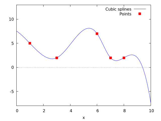
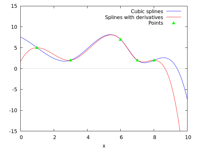
See also: lagrange, linearinterpol, ratinterpol.
lagrange (points) — Function
Computes the polynomial interpolation by the Lagrangian method. Argument points must be either:
a two column matrix, p:matrix([2,4],[5,6],[9,3]),
a list of pairs, p: [[2,4],[5,6],[9,3]],
a list of numbers, p: [4,6,3], in which case the abscissas will be assigned automatically to 1, 2, 3, etc.
In the first two cases the pairs are ordered with respect to the first coordinate before making computations.
With the option argument it is possible to select the name for the independent variable, which is 'x by default; to define another one, write something like varname='z.
Note that when working with high degree polynomials, floating point evaluations are unstable.
See also linearinterpol, cspline, and ratinterpol.
Examples:
maxima
(%i1) load("interpol")$
(%i2) p:[[7,2],[8,2],[1,5],[3,2],[6,7]]$
(%i3) lagrange(p);
(x - 7) (x - 6) (x - 3) (x - 1)
(%o3) -------------------------------
35
(x - 8) (x - 6) (x - 3) (x - 1)
- -------------------------------
12
7 (x - 8) (x - 7) (x - 3) (x - 1)
+ ---------------------------------
30
(x - 8) (x - 7) (x - 6) (x - 1)
- -------------------------------
60
(x - 8) (x - 7) (x - 6) (x - 3)
+ -------------------------------
84
(%i4) define(f(x),%)$
(%i5) expand(map(f,[2.3,5/7,%pi]));
4 3 2
919062 73 %pi 701 %pi 8957 %pi
(%o5) [- 1.567535, ------, ------- - -------- + ---------
84035 420 210 420
5288 %pi 186
- -------- + ---]
105 5
(%i6) plot2d ([f,[discrete,p]], [x,0,10], [style,lines,points],
[legend,"Polynomial","Points"])$
(%i7) lagrange(p, varname=w);
(w - 7) (w - 6) (w - 3) (w - 1)
(%o7) -------------------------------
35
(w - 8) (w - 6) (w - 3) (w - 1)
- -------------------------------
12
7 (w - 8) (w - 7) (w - 3) (w - 1)
+ ---------------------------------
30
(w - 8) (w - 7) (w - 6) (w - 1)
- -------------------------------
60
(w - 8) (w - 7) (w - 6) (w - 3)
+ -------------------------------
84
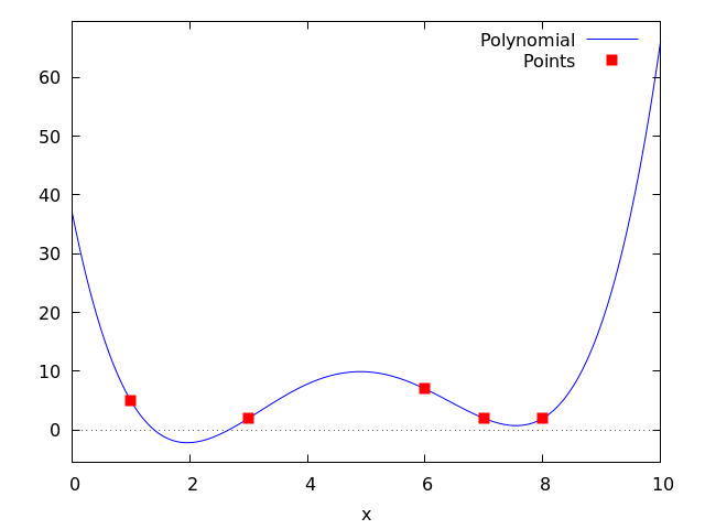
See also: linearinterpol, cspline, ratinterpol.
linearinterpol (points) — Function
Computes the polynomial interpolation by the linear method. Argument points must be either:
a two column matrix, p:matrix([2,4],[5,6],[9,3]),
a list of pairs, p: [[2,4],[5,6],[9,3]],
a list of numbers, p: [4,6,3], in which case the abscissas will be assigned automatically to 1, 2, 3, etc.
In the first two cases the pairs are ordered with respect to the first coordinate before making computations.
With the option argument it is possible to select the name for the independent variable, which is 'x by default; to define another one, write something like varname='z.
See also lagrange, cspline, and ratinterpol.
Examples:
maxima
(%i1) load ("interpol") $
(%i2) p: matrix([7,2],[8,3],[1,5],[3,2],[6,7])$
(%i3) linearinterpol(p);
13 3 x
(%o3) (-- - ---) charfun(x < 3) + charfun((3 <= x) and (x < 6))
2 2
5 x
(--- - 3) + charfun(7 <= x) (x - 5)
3
+ charfun((6 <= x) and (x < 7)) (37 - 5 x)
(%i4) define(f(x),%)$
(%i5) map(f, [7.3,25/7,%pi]);
62 5 %pi
(%o5) [2.3, --, ----- - 3]
21 3
(%i6) float(%);
(%o6) [2.3, 2.9523809523809526, 2.235987755982989]
(%i7) plot2d ([f,[discrete,args(p)]], [x,-5,20], [style,lines,points],
[legend,"Interpolation line","Points"])$
(%i8) lagrange(p, varname=w);
3 (w - 7) (w - 6) (w - 3) (w - 1)
(%o8) ---------------------------------
70
(w - 8) (w - 6) (w - 3) (w - 1)
- -------------------------------
12
7 (w - 8) (w - 7) (w - 3) (w - 1)
+ ---------------------------------
30
(w - 8) (w - 7) (w - 6) (w - 1)
- -------------------------------
60
(w - 8) (w - 7) (w - 6) (w - 3)
+ -------------------------------
84
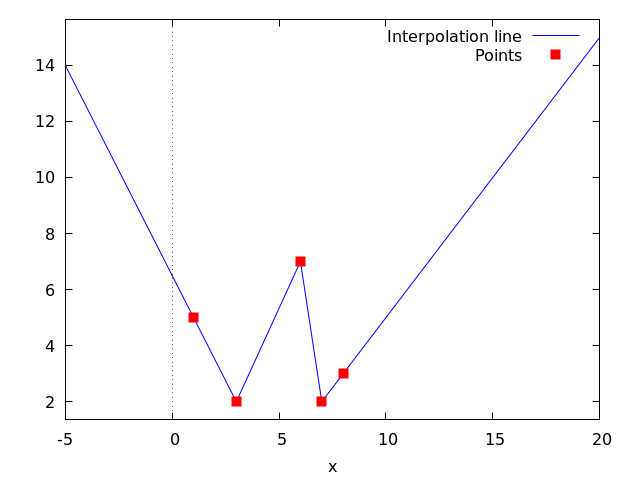
See also: lagrange, cspline, ratinterpol.
ratinterpol (points, numdeg) — Function
Generates a rational interpolator for data given by points and the degree of the numerator being equal to numdeg; the degree of the denominator is calculated automatically. Argument points must be either:
a two column matrix, p:matrix([2,4],[5,6],[9,3]),
a list of pairs, p: [[2,4],[5,6],[9,3]],
a list of numbers, p: [4,6,3], in which case the abscissas will be assigned automatically to 1, 2, 3, etc.
In the first two cases the pairs are ordered with respect to the first coordinate before making computations.
There is one option to fit specific needs:
'varname, default 'x, is the name of the independent variable.
See also lagrange, linearinterpol, cspline, minpack_lsquares, and Package-lbfgs
Examples:
maxima
(%i1) load("interpol")$
(%i2) p:[[7.2,2.5],[8.5,2.1],[1.6,5.1],[3.4,2.4],[6.7,7.9]]$
(%i3) for k:0 thru length(p)-1 do
(%i4) plot2d([ratinterpol(p,k),[discrete,p]], [x,0,9], [y,0,10], [style,lines,points],
[title,concat("Degree of numerator = ",k)], nolegend, gnuplot)$
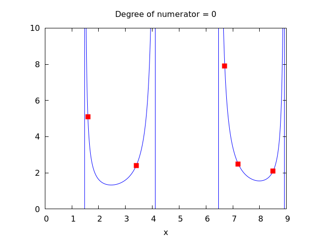
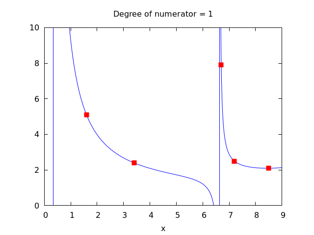
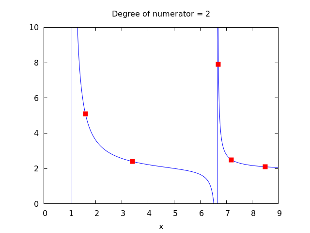
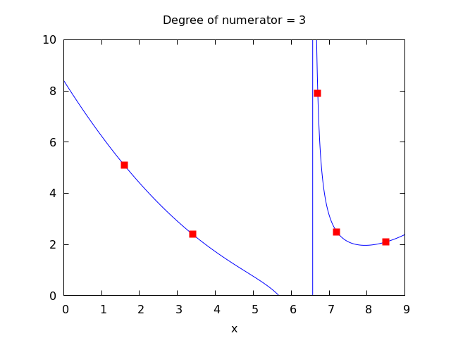
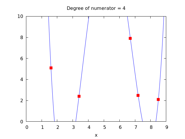
See also: lagrange, linearinterpol, cspline, minpack_lsquares, Package-lbfgs.
lapack
dgeev (A) — Function
Computes the eigenvalues and, optionally, the eigenvectors of a matrix A. All elements of A must be integer or floating point numbers. A must be square (same number of rows and columns). A might or might not be symmetric.
To make use of this function, you must load the LaPack package via
load("lapack").
dgeev(A) computes only the eigenvalues of A.
dgeev(A, right_p, left_p) computes the eigenvalues of A
and the right eigenvectors when $right_p = true$
and the left eigenvectors when $left_p = true$.
A list of three items is returned.
The first item is a list of the eigenvalues.
The second item is false or the matrix of right eigenvectors.
The third item is false or the matrix of left eigenvectors.
The right eigenvector $v_j$ (the $j$-th column of the right eigenvector matrix) satisfies
$$\mathbf{A} v_j = \lambda_j v_j$$
$${\bf A} v_j = \lambda_j v_j $$
where $\lambda_j$ is the corresponding eigenvalue. The left eigenvector $u_j$ (the $j$-th column of the left eigenvector matrix) satisfies
$$u_j^\mathbf{H} \mathbf{A} = \lambda_j u_j^\mathbf{H}$$
$$u_j^{\bf H} {\bf A} = \lambda_j u_j^{\bf H} $$
where
$u_j^\mathbf{H}$
denotes the conjugate transpose of
$u_j.$
For a Maxima function to compute the conjugate transpose, ctranspose.
The computed eigenvectors are normalized to have Euclidean norm equal to 1, and largest component has imaginary part equal to zero.
Example:
maxima
(%i1) load ("lapack")$
(%i2) fpprintprec : 6;
(%o2) 6
(%i3) M : matrix ([9.5, 1.75], [3.25, 10.45]);
[ 9.5 1.75 ]
(%o3) [ ]
[ 3.25 10.45 ]
(%i4) dgeev (M);
(%o4) [[7.54331, 12.4067], false, false]
(%i5) [L, v, u] : dgeev (M, true, true);
[ - 0.666642 - 0.515792 ]
(%o5) [[7.54331, 12.4067], [ ],
[ 0.745378 - 0.856714 ]
[ - 0.856714 - 0.745378 ]
[ ]]
[ 0.515792 - 0.666642 ]
(%i6) D : apply (diag_matrix, L);
[ 7.54331 0 ]
(%o6) [ ]
[ 0 12.4067 ]
(%i7) M . v - v . D;
[ 0.0 - 8.88178e-16 ]
(%o7) [ ]
[ - 8.88178e-16 0.0 ]
(%i8) transpose (u) . M - D . transpose (u);
[ 0.0 - 4.44089e-16 ]
(%o8) [ ]
[ 0.0 0.0 ]
See also: ctranspose.
dgemm (A, B) — Function
Compute the product of two matrices and optionally add the product to a third matrix.
In the simplest form, dgemm(A, B) computes the
product of the two real matrices, A and B.
To make use of this function, you must load the LaPack package via
load("lapack").
In the second form, dgemm computes
$\alpha {\bf A} {\bf B} + \beta {\bf C}$
where
${\bf A},$
${\bf B},$
and
${\bf C}$
are real matrices of the appropriate sizes and
$\alpha$
and
$\beta$
are real numbers. Optionally,
${\bf A}$
and/or
${\bf B}$
can
be transposed before computing the product. The extra parameters are
specified by optional keyword arguments: The keyword arguments are
optional and may be specified in any order. They all take the form
key=val. The keyword arguments are:
C — The matrix
${\bf C}$
that should be added. The default is false,
which means no matrix is added.
alpha — The product of
${\bf A}$
and
${\bf B}$
is multiplied by this value. The
default is 1.
beta — If a matrix
${\bf C}$
is given, this value multiplies
${\bf C}$
before it
is added. The default value is 0, which implies that
${\bf C}$
is not
added, even if
${\bf C}$
is given. Hence, be sure to specify a non-zero
value for
$\beta.$
transpose_a — If true, the transpose of
${\bf A}$
is used instead of
${\bf A}$
for the product. The default is false.
transpose_b — If true, the transpose of
${\bf B}$
is used instead of
${\bf B}$
for the product. The default is false.
maxima
(%i1) load ("lapack")$
(%i2) A : matrix([1,2,3],[4,5,6],[7,8,9]);
[ 1 2 3 ]
[ ]
(%o2) [ 4 5 6 ]
[ ]
[ 7 8 9 ]
(%i3) B : matrix([-1,-2,-3],[-4,-5,-6],[-7,-8,-9]);
[ - 1 - 2 - 3 ]
[ ]
(%o3) [ - 4 - 5 - 6 ]
[ ]
[ - 7 - 8 - 9 ]
(%i4) C : matrix([3,2,1],[6,5,4],[9,8,7]);
[ 3 2 1 ]
[ ]
(%o4) [ 6 5 4 ]
[ ]
[ 9 8 7 ]
(%i5) dgemm(A,B);
[ - 30.0 - 36.0 - 42.0 ]
[ ]
(%o5) [ - 66.0 - 81.0 - 96.0 ]
[ ]
[ - 102.0 - 126.0 - 150.0 ]
(%i6) A . B;
[ - 30 - 36 - 42 ]
[ ]
(%o6) [ - 66 - 81 - 96 ]
[ ]
[ - 102 - 126 - 150 ]
(%i7) dgemm(A,B,transpose_a=true);
[ - 66.0 - 78.0 - 90.0 ]
[ ]
(%o7) [ - 78.0 - 93.0 - 108.0 ]
[ ]
[ - 90.0 - 108.0 - 126.0 ]
(%i8) transpose(A) . B;
[ - 66 - 78 - 90 ]
[ ]
(%o8) [ - 78 - 93 - 108 ]
[ ]
[ - 90 - 108 - 126 ]
(%i9) dgemm(A,B,c=C,beta=1);
[ - 27.0 - 34.0 - 41.0 ]
[ ]
(%o9) [ - 60.0 - 76.0 - 92.0 ]
[ ]
[ - 93.0 - 118.0 - 143.0 ]
(%i10) A . B + C;
[ - 27 - 34 - 41 ]
[ ]
(%o10) [ - 60 - 76 - 92 ]
[ ]
[ - 93 - 118 - 143 ]
(%i11) dgemm(A,B,c=C,beta=1, alpha=-1);
[ 33.0 38.0 43.0 ]
[ ]
(%o11) [ 72.0 86.0 100.0 ]
[ ]
[ 111.0 134.0 157.0 ]
(%i12) -A . B + C;
[ 33 38 43 ]
[ ]
(%o12) [ 72 86 100 ]
[ ]
[ 111 134 157 ]
dgeqrf (A) — Function
Computes the QR decomposition of the matrix A. All elements of A must be integer or floating point numbers. A may or may not have the same number of rows and columns.
To make use of this function, you must load the LaPack package via
load("lapack").
The real square matrix $\mathbf{A}$ can be decomposed as
$$\mathbf{A} = \mathbf{Q}\mathbf{R}$$
$${\bf A} = {\bf Q} {\bf R}$$
where ${\bf Q}$ is a square orthogonal matrix with the same number of rows as $\mathbf{A}$ and ${\bf R}$ is an upper triangular matrix and is the same size as ${\bf A}.$
A list of two items is returned. The first item is the matrix ${\bf Q}.$ The second item is the matrix ${\bf R},$ The product $Q . R$, where “.” is the noncommutative multiplication operator, is equal to A (ignoring floating point round-off errors).
maxima
(%i1) load ("lapack")$
(%i2) fpprintprec : 6;
(%o2) 6
(%i3) M : matrix ([1, -3.2, 8], [-11, 2.7, 5.9]);
[ 1 - 3.2 8 ]
(%o3) [ ]
[ - 11 2.7 5.9 ]
(%i4) [q, r] : dgeqrf (M);
[ - 0.0905357 0.995893 ]
(%o4) [[ ],
[ 0.995893 0.0905357 ]
[ - 11.0454 2.97863 5.15148 ]
[ ]]
[ 0.0 - 2.94241 8.50131 ]
(%i5) q . r - M;
[ - 7.77156e-16 1.77636e-15 - 8.88178e-16 ]
(%o5) [ ]
[ 0.0 - 1.33227e-15 8.88178e-16 ]
(%i6) mat_norm (%, 1);
(%o6) 3.10862e-15
dgesv (A, b) — Function
Computes the solution x of the linear equation ${\bf A} x = b,$ where ${\bf A}$ is a square matrix, and $b$ is a matrix of the same number of rows as ${\bf A}$ and any number of columns. The return value $x$ is the same size as $b$.
To make use of this function, you must load the LaPack package via
load("lapack").
The elements of A and b must evaluate to real floating point numbers via float;
thus elements may be any numeric type, symbolic numerical constants, or expressions which evaluate to floats.
The elements of x are always floating point numbers.
All arithmetic is carried out as floating point operations.
dgesv computes the solution via the LU decomposition of A.
Examples:
dgesv computes the solution of the linear equation $A x = b$.
maxima
(%i1) load("lapack")$
(%i2) A : matrix ([1, -2.5], [0.375, 5]);
[ 1 - 2.5 ]
(%o2) [ ]
[ 0.375 5 ]
(%i3) b : matrix ([1.75], [-0.625]);
[ 1.75 ]
(%o3) [ ]
[ - 0.625 ]
(%i4) x : dgesv (A, b);
[ 1.2105263157894737 ]
(%o4) [ ]
[ - 0.21578947368421053 ]
(%i5) dlange (inf_norm, b - A . x);
(%o5) 0.0
b is a matrix with the same number of rows as A and any number of columns. x is the same size as b.
maxima
(%i1) load ("lapack")$
(%i2) A : matrix ([1, -0.15], [1.82, 2]);
[ 1 - 0.15 ]
(%o2) [ ]
[ 1.82 2 ]
(%i3) b : matrix ([3.7, 1, 8], [-2.3, 5, -3.9]);
[ 3.7 1 8 ]
(%o3) [ ]
[ - 2.3 5 - 3.9 ]
(%i4) x : dgesv (A, b);
(%o4)
[ 3.1038275406951175 1.2098548174219095 6.7817861856577215 ]
[ ]
[ - 3.974483062032557 1.3990321161460624 - 8.121425428948527 ]
(%i5) dlange (inf_norm, b - A . x);
(%o5) 1.1102230246251565e-15
The elements of A and b must evaluate to real floating point numbers.
maxima
(%i1) load ("lapack")$
(%i2) A : matrix ([5, -%pi], [1b0, 11/17]);
[ 5 - %pi ]
[ ]
(%o2) [ 11 ]
[ 1.0b0 -- ]
[ 17 ]
(%i3) b : matrix ([%e], [sin(1)]);
[ %e ]
(%o3) [ ]
[ sin(1) ]
(%i4) x : dgesv (A, b);
[ 0.6903756431559864 ]
(%o4) [ ]
[ 0.23351098255295172 ]
(%i5) dlange (inf_norm, b - A . x);
(%o5) 2.220446049250313e-16
dgesvd (A) — Function
Computes the singular value decomposition (SVD) of a matrix A, comprising the singular values and, optionally, the left and right singular vectors. All elements of A must be integer or floating point numbers. A might or might not be square (same number of rows and columns).
To make use of this function, you must load the LaPack package via
load("lapack").
Let $m$ be the number of rows, and $n$ the number of columns of A. The singular value decomposition of $\mathbf{A}$ comprises three matrices, $\mathbf{U},$ $\mathbf{\Sigma},$ and $\mathbf{V},$ such that
$$\mathbf{A} = \mathbf{U} \mathbf{\Sigma} \mathbf{V}^T$$
$${\bf A} = {\bf U} {\bf \Sigma} {\bf V}^T$$
where $\mathbf{U}$ is an $m$-by-$m$ unitary matrix, $\mathbf{\Sigma}$ is an $m$-by-$n$ diagonal matrix, and $\mathbf{V}$ is an $n$-by-$n$ unitary matrix.
Let
$\mathbf{\sigma}i$
be a diagonal element of
$\mathbf{\Sigma},$
that is,
$\mathbf{\Sigma}{ii} = \sigma_i.$
The elements
$\sigma_i$
are the so-called singular values of
$\mathbf{A};$
these are real and nonnegative, and returned in descending order.
The first
$\min(m, n)$
columns of
$\mathbf{U}$
and
$\mathbf{V}$
are the left and right singular vectors of
$\mathbf{A}.$
Note that dgesvd returns the transpose of
$\mathbf{V},$
not
$\mathbf{V}$
itself.
dgesvd(A) computes only the singular values of A.
dgesvd(A, left_p, right_p) computes the singular values of A
and the left singular vectors when $left_p = true$
and the right singular vectors when $right_p = true$.
A list of three items is returned.
The first item is a list of the singular values.
The second item is false or the matrix of left singular vectors.
The third item is false or the matrix of right singular vectors.
Example:
maxima
(%i1) load ("lapack")$
(%i2) fpprintprec : 6;
(%o2) 6
(%i3) M: matrix([1, 2, 3], [3.5, 0.5, 8], [-1, 2, -3], [4, 9, 7]);
[ 1 2 3 ]
[ ]
[ 3.5 0.5 8 ]
(%o3) [ ]
[ - 1 2 - 3 ]
[ ]
[ 4 9 7 ]
(%i4) dgesvd (M);
(%o4) [[14.4744, 6.38637, 0.452547], false, false]
(%i5) [sigma, U, VT] : dgesvd (M, true, true);
(%o5) [[14.4744, 6.38637, 0.452547],
[ - 0.256731 0.00816168 0.959029 - 0.119523 ]
[ ]
[ - 0.526456 0.672116 - 0.206236 - 0.478091 ]
[ ],
[ 0.107997 - 0.532278 - 0.0708315 - 0.83666 ]
[ ]
[ - 0.803287 - 0.514659 - 0.180867 0.239046 ]
[ - 0.374486 - 0.538209 - 0.755044 ]
[ ]
[ 0.130623 - 0.836799 0.5317 ]]
[ ]
[ - 0.917986 0.100488 0.383672 ]
(%i6) m : length (U);
(%o6) 4
(%i7) n : length (VT);
(%o7) 3
(%i8) Sigma:
genmatrix(lambda ([i, j], if i=j then sigma[i] else 0),
m, n);
[ 14.4744 0 0 ]
[ ]
[ 0 6.38637 0 ]
(%o8) [ ]
[ 0 0 0.452547 ]
[ ]
[ 0 0 0 ]
(%i9) U . Sigma . VT - M;
[ 1.11022e-15 0.0 1.77636e-15 ]
[ ]
[ 1.33227e-15 1.66533e-15 0.0 ]
(%o9) [ ]
[ - 4.44089e-16 - 8.88178e-16 4.44089e-16 ]
[ ]
[ 8.88178e-16 1.77636e-15 8.88178e-16 ]
(%i10) transpose (U) . U;
[ 1.0 5.55112e-17 2.498e-16 2.77556e-17 ]
[ ]
[ 5.55112e-17 1.0 5.55112e-17 4.16334e-17 ]
(%o10) [ ]
[ 2.498e-16 5.55112e-17 1.0 - 2.08167e-16 ]
[ ]
[ 2.77556e-17 4.16334e-17 - 2.08167e-16 1.0 ]
(%i11) VT . transpose (VT);
[ 1.0 0.0 - 5.55112e-17 ]
[ ]
(%o11) [ 0.0 1.0 5.55112e-17 ]
[ ]
[ - 5.55112e-17 5.55112e-17 1.0 ]
dlange (norm, A) — Function
Computes a norm or norm-like function of the matrix A. If
A is a real matrix, use dlange. For a matrix with
complex elements, use zlange.
To make use of this function, you must load the LaPack package via
load("lapack").
norm specifies the kind of norm to be computed:
max — Compute $\max(|{\bf A}{ij}|)$ where $i$ and $j$ range over the rows and columns, respectively, of ${\bf A}.$ Note that this function is not a proper matrix norm. one_norm — Compute the $L_1$ norm of ${\bf A},$ that is, the maximum of the sum of the absolute value of elements in each column. inf_norm — Compute the $L\infty$ norm of ${\bf A},$ that is, the maximum of the sum of the absolute value of elements in each row. frobenius — Compute the Frobenius norm of ${\bf A},$ that is, the square root of the sum of squares of the matrix elements.
zgeev (A) — Function
Like dgeev, but the matrix
${\bf A}$
is complex.
To make use of this function, you must load the LaPack package via
load("lapack").
See also: dgeev.
zheev (A) — Function
Like dgeev, but the matrix
${\bf A}$
is assumed to be a square
complex Hermitian matrix. If eigvec_p is true, then the
eigenvectors of the matrix are also computed.
To make use of this function, you must load the LaPack package via
load("lapack").
No check is made that the matrix ${\bf A}$ is, in fact, Hermitian.
A list of two items is returned, as in dgeev: a list of
eigenvalues, and false or the matrix of the eigenvectors.
maxima
(%i1) load("lapack")$
(%i2) M: matrix(
[9.14 +%i*0.00 , -4.37 -%i*9.22 , -1.98 -%i*1.72 , -8.96 -%i*9.50],
[-4.37 +%i*9.22 , -3.35 +%i*0.00 , 2.25 -%i*9.51 , 2.57 +%i*2.40],
[-1.98 +%i*1.72 , 2.25 +%i*9.51 , -4.82 +%i*0.00 , -3.24 +%i*2.04],
[-8.96 +%i*9.50 , 2.57 -%i*2.40 , -3.24 -%i*2.04 , 8.44 +%i*0.00]);
[ 9.14 ] [ - 9.22 %i - 4.37 ]
[ ] [ ]
[ 9.22 %i - 4.37 ] [ - 3.35 ]
(%o2) Col 1 = [ ] Col 2 = [ ]
[ 1.72 %i - 1.98 ] [ 9.51 %i + 2.25 ]
[ ] [ ]
[ 9.5 %i - 8.96 ] [ 2.57 - 2.4 %i ]
[ - 1.72 %i - 1.98 ] [ - 9.5 %i - 8.96 ]
[ ] [ ]
[ 2.25 - 9.51 %i ] [ 2.4 %i + 2.57 ]
Col 3 = [ ] Col 4 = [ ]
[ - 4.82 ] [ 2.04 %i - 3.24 ]
[ ] [ ]
[ - 2.04 %i - 3.24 ] [ 8.44 ]
(%i3) zheev(M);
(%o3) [[- 16.004746472094734, - 6.764970154793324,
6.6657114535070985, 25.51400517338097], false]
(%i4) E: zheev(M,true)$
(%i5) E[1];
(%o5) [- 16.004746472094737, - 6.764970154793325,
6.665711453507101, 25.514005173380962]
(%i6) E[2];
[ 0.26746505331727455 %i + 0.21754535866650165 ]
[ ]
[ 0.002696730886619885 %i + 0.6968836773391712 ]
(%o6) Col 1 = [ ]
[ - 0.6082406376714117 %i - 0.012106142926979313 ]
[ ]
[ 0.15930818580950368 ]
[ 0.26449374706674444 %i + 0.4773693349937472 ]
[ ]
[ - 0.28523890360316206 %i - 0.14143627420116733 ]
Col 2 = [ ]
[ 0.2654607680986639 %i + 0.44678181171841735 ]
[ ]
[ 0.5750762708542709 ]
[ 0.28106497673059216 %i - 0.13352639282451817 ]
[ ]
[ 0.28663101328695556 %i - 0.4536971347853274 ]
Col 3 = [ ]
[ - 0.29336843237542953 %i - 0.49549724255410565 ]
[ ]
[ 0.5325337537576771 ]
[ - 0.5737316575503476 %i - 0.39661467994277055 ]
[ ]
[ 0.018265026190214573 %i + 0.35305577043870173 ]
Col 4 = [ ]
[ 0.16737009000854253 %i + 0.01476684746229564 ]
[ ]
[ 0.6002632636961784 ]
See also: dgeev.
lbfgs
lbfgs (FOM, X, X0, epsilon, iprint) — Function
Finds an approximate solution of the unconstrained minimization of the figure of merit FOM over the list of variables X, starting from initial estimates X0, such that $norm(grad(FOM)) < epsilon*max(1, norm(X))$.
grad, if present, is the gradient of FOM with respect to the variables X. grad may be a list or a function that returns a list, with one element for each element of X. If not present, the gradient is computed automatically by symbolic differentiation. If FOM is a function, the gradient grad must be supplied by the user.
The algorithm applied is a limited-memory quasi-Newton (BFGS) algorithm [1]. It is called a limited-memory method because a low-rank approximation of the Hessian matrix inverse is stored instead of the entire Hessian inverse. Each iteration of the algorithm is a line search, that is, a search along a ray in the variables X, with the search direction computed from the approximate Hessian inverse. The FOM is always decreased by a successful line search. Usually (but not always) the norm of the gradient of FOM also decreases.
iprint controls progress messages printed by lbfgs.
iprint[1] — iprint[1] controls the frequency of progress messages.
iprint[1] < 0 — No progress messages.
iprint[1] = 0 — Messages at the first and last iterations.
iprint[1] > 0 — Print a message every iprint[1] iterations.
iprint[2] — iprint[2] controls the verbosity of progress messages.
iprint[2] = 0 — Print out iteration count, number of evaluations of FOM, value of FOM,
norm of the gradient of FOM, and step length.
iprint[2] = 1 — Same as iprint[2] = 0, plus X0 and the gradient of FOM evaluated at X0.
iprint[2] = 2 — Same as iprint[2] = 1, plus values of X at each iteration.
iprint[2] = 3 — Same as iprint[2] = 2, plus the gradient of FOM at each iteration.
The columns printed by lbfgs are the following.
I — Number of iterations. It is incremented for each line search. NFN — Number of evaluations of the figure of merit. FUNC — Value of the figure of merit at the end of the most recent line search. GNORM — Norm of the gradient of the figure of merit at the end of the most recent line search. STEPLENGTH — An internal parameter of the search algorithm.
Additional information concerning details of the algorithm are found in the comments of the original Fortran code [2].
See also lbfgs_nfeval_max and lbfgs_005fncorrections.
References:
[1] D. Liu and J. Nocedal. “On the limited memory BFGS method for large scale optimization”. Mathematical Programming B 45:503–528 (1989)
[2] https://www.netlib.org/opt/lbfgs_um.shar
Examples:
The same FOM as computed by FGCOMPUTE in the program sdrive.f in the LBFGS package from Netlib. Note that the variables in question are subscripted variables. The FOM has an exact minimum equal to zero at $u[k] = 1$ for $k = 1, …, 8$.
(%i1) load ("lbfgs")$
(%i2) t1[j] := 1 - u[j];
(%o2) t1 := 1 - u
j j
(%i3) t2[j] := 10*(u[j + 1] - u[j]^2);
2
(%o3) t2 := 10 (u - u )
j j + 1 j
(%i4) n : 8;
(%o4) 8
(%i5) FOM : sum (t1[2*j - 1]^2 + t2[2*j - 1]^2, j, 1, n/2);
2 2 2 2 2 2
(%o5) 100 (u - u ) + (1 - u ) + 100 (u - u ) + (1 - u )
8 7 7 6 5 5
2 2 2 2 2 2
+ 100 (u - u ) + (1 - u ) + 100 (u - u ) + (1 - u )
4 3 3 2 1 1
(%i6) lbfgs (FOM, '[u[1],u[2],u[3],u[4],u[5],u[6],u[7],u[8]],
[-1.2, 1, -1.2, 1, -1.2, 1, -1.2, 1], 1e-3, [1, 0]);
*************************************************
N= 8 NUMBER OF CORRECTIONS=25
INITIAL VALUES
F= 9.680000000000000D+01 GNORM= 4.657353755084533D+02
*************************************************
I NFN FUNC GNORM STEPLENGTH
1 3 1.651479526340304D+01 4.324359291335977D+00 7.926153934390631D-04
2 4 1.650209316638371D+01 3.575788161060007D+00 1.000000000000000D+00
3 5 1.645461701312851D+01 6.230869903601577D+00 1.000000000000000D+00
4 6 1.636867301275588D+01 1.177589920974980D+01 1.000000000000000D+00
5 7 1.612153014409201D+01 2.292797147151288D+01 1.000000000000000D+00
6 8 1.569118407390628D+01 3.687447158775571D+01 1.000000000000000D+00
7 9 1.510361958398942D+01 4.501931728123679D+01 1.000000000000000D+00
8 10 1.391077875774293D+01 4.526061463810630D+01 1.000000000000000D+00
9 11 1.165625686278198D+01 2.748348965356907D+01 1.000000000000000D+00
10 12 9.859422687859144D+00 2.111494974231706D+01 1.000000000000000D+00
11 13 7.815442521732282D+00 6.110762325764183D+00 1.000000000000000D+00
12 15 7.346380905773044D+00 2.165281166715009D+01 1.285316401779678D-01
13 16 6.330460634066464D+00 1.401220851761508D+01 1.000000000000000D+00
14 17 5.238763939854303D+00 1.702473787619218D+01 1.000000000000000D+00
15 18 3.754016790406625D+00 7.981845727632704D+00 1.000000000000000D+00
16 20 3.001238402313225D+00 3.925482944745832D+00 2.333129631316462D-01
17 22 2.794390709722064D+00 8.243329982586480D+00 2.503577283802312D-01
18 23 2.563783562920545D+00 1.035413426522664D+01 1.000000000000000D+00
19 24 2.019429976373283D+00 1.065187312340952D+01 1.000000000000000D+00
20 25 1.428003167668592D+00 2.475962450735100D+00 1.000000000000000D+00
21 27 1.197874264859232D+00 8.441707983339661D+00 4.303451060697367D-01
22 28 9.023848942003913D-01 1.113189216665625D+01 1.000000000000000D+00
23 29 5.508226405855795D-01 2.380830599637816D+00 1.000000000000000D+00
24 31 3.902893258879521D-01 5.625595817143044D+00 4.834988416747262D-01
25 32 3.207542206881058D-01 1.149444645298493D+01 1.000000000000000D+00
26 33 1.874468266118200D-01 3.632482152347445D+00 1.000000000000000D+00
27 34 9.575763380282112D-02 4.816497449000391D+00 1.000000000000000D+00
28 35 4.085145106760390D-02 2.087009347116811D+00 1.000000000000000D+00
29 36 1.931106005512628D-02 3.886818624052740D+00 1.000000000000000D+00
30 37 6.894000636920714D-03 3.198505769992936D+00 1.000000000000000D+00
31 38 1.443296008850287D-03 1.590265460381961D+00 1.000000000000000D+00
32 39 1.571766574930155D-04 3.098257002223532D-01 1.000000000000000D+00
33 40 1.288011779655132D-05 1.207784334505595D-02 1.000000000000000D+00
34 41 1.806140190993455D-06 4.587890258846915D-02 1.000000000000000D+00
35 42 1.769004612050548D-07 1.790537363138099D-02 1.000000000000000D+00
36 43 3.312164244118216D-10 6.782068546986653D-04 1.000000000000000D+00
\halign{\hfil\tt#&\quad\hfil\tt#\quad&\tt#\hfil\quad&\tt#\hfil\quad&\tt#\hfil\cr I& NFN& FUNC& GNORM& STEPLENGTH\cr &&&&\cr 1& 3& 1.651479526340304D+01& 4.324359291335977D+00& 7.926153934390631D-04\cr 2& 4& 1.650209316638371D+01& 3.575788161060007D+00& 1.000000000000000D+00\cr 3& 5& 1.645461701312851D+01& 6.230869903601577D+00& 1.000000000000000D+00\cr 4& 6& 1.636867301275588D+01& 1.177589920974980D+01& 1.000000000000000D+00\cr 5& 7& 1.612153014409201D+01& 2.292797147151288D+01& 1.000000000000000D+00\cr 6& 8& 1.569118407390628D+01& 3.687447158775571D+01& 1.000000000000000D+00\cr 7& 9& 1.510361958398942D+01& 4.501931728123680D+01& 1.000000000000000D+00\cr 8&10& 1.391077875774294D+01& 4.526061463810632D+01& 1.000000000000000D+00\cr 9&11& 1.165625686278198D+01& 2.748348965356917D+01& 1.000000000000000D+00\cr 10&12& 9.859422687859137D+00& 2.111494974231644D+01& 1.000000000000000D+00\cr 11&13& 7.815442521732281D+00& 6.110762325766556D+00& 1.000000000000000D+00\cr 12&15& 7.346380905773160D+00& 2.165281166714631D+01& 1.285316401779533D-01\cr 13&16& 6.330460634066370D+00& 1.401220851762050D+01& 1.000000000000000D+00\cr 14&17& 5.238763939851439D+00& 1.702473787613255D+01& 1.000000000000000D+00\cr 15&18& 3.754016790406701D+00& 7.981845727704576D+00& 1.000000000000000D+00\cr 16&20& 3.001238402309352D+00& 3.925482944716691D+00& 2.333129631296807D-01\cr 17&22& 2.794390709718290D+00& 8.243329982546473D+00& 2.503577283782332D-01\cr 18&23& 2.563783562918759D+00& 1.035413426521790D+01& 1.000000000000000D+00\cr 19&24& 2.019429976377856D+00& 1.065187312346769D+01& 1.000000000000000D+00\cr 20&25& 1.428003167670903D+00& 2.475962450826961D+00& 1.000000000000000D+00\cr 21&27& 1.197874264861340D+00& 8.441707983493810D+00& 4.303451060808756D-01\cr 22&28& 9.023848941942773D-01& 1.113189216635162D+01& 1.000000000000000D+00\cr 23&29& 5.508226405863770D-01& 2.380830600326308D+00& 1.000000000000000D+00\cr 24&31& 3.902893258815567D-01& 5.625595816584421D+00& 4.834988416524465D-01\cr 25&32& 3.207542206990315D-01& 1.149444645416472D+01& 1.000000000000000D+00\cr 26&33& 1.874468266362791D-01& 3.632482152880997D+00& 1.000000000000000D+00\cr 27&34& 9.575763380706598D-02& 4.816497446154354D+00& 1.000000000000000D+00\cr 28&35& 4.085145107543406D-02& 2.087009350166495D+00& 1.000000000000000D+00\cr 29&36& 1.931106001379290D-02& 3.886818608498966D+00& 1.000000000000000D+00\cr 30&37& 6.894000721499670D-03& 3.198505796342214D+00& 1.000000000000000D+00\cr 31&38& 1.443296033051864D-03& 1.590265471025043D+00& 1.000000000000000D+00\cr 32&39& 1.571766603154336D-04& 3.098257063980634D-01& 1.000000000000000D+00\cr 33&40& 1.288011776581970D-05& 1.207784183577257D-02& 1.000000000000000D+00\cr 34&41& 1.806140173752971D-06& 4.587890233385193D-02& 1.000000000000000D+00\cr 35&42& 1.769004645459358D-07& 1.790537375052208D-02& 1.000000000000000D+00\cr 36&43& 3.312164100763217D-10& 6.782068426119681D-04& 1.000000000000000D+00\cr }
THE MINIMIZATION TERMINATED WITHOUT DETECTING ERRORS.
IFLAG = 0
(%o6) [u = 1.000005339816132, u = 1.000009942840108,
1 2
u = 1.000005339816132, u = 1.000009942840108,
3 4
u = 1.000005339816132, u = 1.000009942840108,
5 6
u = 1.000005339816132, u = 1.000009942840108]
7 8
A regression problem.
The FOM is the mean square difference between the predicted value $F(X[i])$
and the observed value $Y[i]$.
The function $F$ is a bounded monotone function (a so-called “sigmoidal” function).
In this example, lbfgs computes approximate values for the parameters of $F$
and plot2d displays a comparison of $F$ with the observed data.
(%i1) load ("lbfgs")$
(%i2) FOM : '((1/length(X))*sum((F(X[i]) - Y[i])^2, i, 1,
length(X)));
2
sum((F(X ) - Y ) , i, 1, length(X))
i i
(%o2) -----------------------------------
length(X)
(%i3) X : [1, 2, 3, 4, 5];
(%o3) [1, 2, 3, 4, 5]
(%i4) Y : [0, 0.5, 1, 1.25, 1.5];
(%o4) [0, 0.5, 1, 1.25, 1.5]
(%i5) F(x) := A/(1 + exp(-B*(x - C)));
A
(%o5) F(x) := ----------------------
1 + exp((- B) (x - C))
(%i6) ''FOM;
A 2 A 2
(%o6) ((----------------- - 1.5) + (----------------- - 1.25)
- B (5 - C) - B (4 - C)
%e + 1 %e + 1
A 2 A 2
+ (----------------- - 1) + (----------------- - 0.5)
- B (3 - C) - B (2 - C)
%e + 1 %e + 1
2
A
+ --------------------)/5
- B (1 - C) 2
(%e + 1)
(%i7) estimates : lbfgs (FOM, '[A, B, C], [1, 1, 1], 1e-4, [1, 0]);
*************************************************
N= 3 NUMBER OF CORRECTIONS=25
INITIAL VALUES
F= 1.348738534246918D-01 GNORM= 2.000215531936760D-01
*************************************************
I NFN FUNC GNORM STEPLENGTH
1 3 1.177820636622582D-01 9.893138394953992D-02 8.554435968992371D-01
2 6 2.302653892214013D-02 1.180098521565904D-01 2.100000000000000D+01
3 8 1.496348495303004D-02 9.611201567691624D-02 5.257340567840710D-01
4 9 7.900460841091138D-03 1.325041647391314D-02 1.000000000000000D+00
5 10 7.314495451266914D-03 1.510670810312226D-02 1.000000000000000D+00
6 11 6.750147275936668D-03 1.914964958023037D-02 1.000000000000000D+00
7 12 5.850716021108202D-03 1.028089194579382D-02 1.000000000000000D+00
8 13 5.778664230657800D-03 3.676866074532179D-04 1.000000000000000D+00
9 14 5.777818823650780D-03 3.010740179797108D-04 1.000000000000000D+00
\halign{\hfil\tt#&\quad\hfil\tt#\quad&\tt#\hfil\quad&\tt#\hfil\quad&\tt#\hfil\cr I& NFN& FUNC& GNORM& STEPLENGTH\cr &&&&\cr 1& 3&1.177820636622582D-01& 9.893138394953992D-02& 8.554435968992371D-01\cr 2& 6&2.302653892214013D-02& 1.180098521565904D-01& 2.100000000000000D+01\cr 3& 8&1.496348495303004D-02& 9.611201567691624D-02& 5.257340567840710D-01\cr 4& 9&7.900460841091138D-03& 1.325041647391314D-02& 1.000000000000000D+00\cr 5& 10&7.314495451266914D-03& 1.510670810312226D-02& 1.000000000000000D+00\cr 6& 11&6.750147275936668D-03& 1.914964958023037D-02& 1.000000000000000D+00\cr 7& 12&5.850716021108202D-03& 1.028089194579382D-02& 1.000000000000000D+00\cr 8& 13&5.778664230657800D-03& 3.676866074532179D-04& 1.000000000000000D+00\cr 9& 14&5.777818823650780D-03& 3.010740179797108D-04& 1.000000000000000D+00\cr }
THE MINIMIZATION TERMINATED WITHOUT DETECTING ERRORS.
IFLAG = 0
(%o7) [A = 1.461933911464101, B = 1.601593973254801,
C = 2.528933072164855]
(%i8) plot2d ([F(x), [discrete, X, Y]], [x, -1, 6]), ''estimates;
(%o8)
Gradient of FOM is specified (instead of computing it automatically).
Both the FOM and its gradient are passed as functions to lbfgs.
(%i1) load ("lbfgs")$
(%i2) F(a, b, c) := (a - 5)^2 + (b - 3)^4 + (c - 2)^6$
(%i3) define(F_grad(a, b, c),
map (lambda ([x], diff (F(a, b, c), x)), [a, b, c]))$
(%i4) estimates : lbfgs ([F, F_grad],
[a, b, c], [0, 0, 0], 1e-4, [1, 0]);
*************************************************
N= 3 NUMBER OF CORRECTIONS=25
INITIAL VALUES
F= 1.700000000000000D+02 GNORM= 2.205175729958953D+02
*************************************************
I NFN FUNC GNORM STEPLENGTH
1 2 6.632967565917637D+01 6.498411132518770D+01 4.534785987412505D-03
2 3 4.368890936228036D+01 3.784147651974131D+01 1.000000000000000D+00
3 4 2.685298972775191D+01 1.640262125898520D+01 1.000000000000000D+00
4 5 1.909064767659852D+01 9.733664001790506D+00 1.000000000000000D+00
5 6 1.006493272061515D+01 6.344808151880209D+00 1.000000000000000D+00
6 7 1.215263596054292D+00 2.204727876126877D+00 1.000000000000000D+00
7 8 1.080252896385329D-02 1.431637116951845D-01 1.000000000000000D+00
8 9 8.407195124830860D-03 1.126344579730008D-01 1.000000000000000D+00
9 10 5.022091686198525D-03 7.750731829225275D-02 1.000000000000000D+00
10 11 2.277152808939775D-03 5.032810859286796D-02 1.000000000000000D+00
11 12 6.489384688303218D-04 1.932007150271009D-02 1.000000000000000D+00
12 13 2.075791943844547D-04 6.964319310814365D-03 1.000000000000000D+00
13 14 7.349472666162258D-05 4.017449067849554D-03 1.000000000000000D+00
14 15 2.293617477985238D-05 1.334590390856715D-03 1.000000000000000D+00
15 16 7.683645404048675D-06 6.011057038099202D-04 1.000000000000000D+00
\halign{\hfil\tt#&\quad\hfil\tt#\quad&\tt#\hfil\quad&\tt#\hfil\quad&\tt#\hfil\cr I& NFN& FUNC& GNORM& STEPLENGTH\cr &&&&\cr 1& 2& 6.632967565917637D+01& 6.498411132518770D+01& 4.534785987412505D-03\cr 2& 3& 4.368890936228036D+01& 3.784147651974131D+01& 1.000000000000000D+00\cr 3& 4& 2.685298972775191D+01& 1.640262125898520D+01& 1.000000000000000D+00\cr 4& 5& 1.909064767659852D+01& 9.733664001790506D+00& 1.000000000000000D+00\cr 5& 6& 1.006493272061515D+01& 6.344808151880209D+00& 1.000000000000000D+00\cr 6& 7& 1.215263596054292D+00& 2.204727876126877D+00& 1.000000000000000D+00\cr 7& 8& 1.080252896385329D-02& 1.431637116951845D-01& 1.000000000000000D+00\cr 8& 9& 8.407195124830860D-03& 1.126344579730008D-01& 1.000000000000000D+00\cr 9& 10& 5.022091686198525D-03& 7.750731829225275D-02& 1.000000000000000D+00\cr 10& 11& 2.277152808939775D-03& 5.032810859286796D-02& 1.000000000000000D+00\cr 11& 12& 6.489384688303218D-04& 1.932007150271009D-02& 1.000000000000000D+00\cr 12& 13& 2.075791943844547D-04& 6.964319310814365D-03& 1.000000000000000D+00\cr 13& 14& 7.349472666162258D-05& 4.017449067849554D-03& 1.000000000000000D+00\cr 14& 15& 2.293617477985238D-05& 1.334590390856715D-03& 1.000000000000000D+00\cr 15& 16& 7.683645404048675D-06& 6.011057038099202D-04& 1.000000000000000D+00\cr }
THE MINIMIZATION TERMINATED WITHOUT DETECTING ERRORS.
IFLAG = 0
(%o4) [a = 5.000086823042934, b = 3.052395429705181,
c = 1.927980629919583]
See also: lbfgs_nfeval_max, lbfgs_ncorrections.
lbfgs_ncorrections — Variable
Default value: 25
lbfgs_ncorrections is the number of corrections applied
to the approximate inverse Hessian matrix which is maintained by lbfgs.
lbfgs_nfeval_max — Variable
Default value: 100
lbfgs_nfeval_max is the maximum number of evaluations of the figure of merit (FOM) in lbfgs.
When lbfgs_nfeval_max is reached,
lbfgs returns the result of the last successful line search.
levin
bflevin_u_sum (a, n, n_0) — Function
Estimate sum(a(n), n, n_0, inf) using the
Levin u-transform in bigfloat arithmetic.
bflevin_u_sum attempts to return the sum of the infinite series
with a precision given by the global variable fpprec using bigfloat arithmetic.
See levin_options for options to control this function.
bflevin_u_sum uses an adaptive algorithm to increase both the number of
terms and the bigfloat precision used for internal calculations
until the estimated error is acceptable.
load("levin") loads this function.
See Examples for levin for examples.
See also: fpprec, levin_options, Examples-for-levin.
Function: levin_options
Function bflevin_u_sum attempts to return the sum of an infinite series
with a precision given by the global variable fpprec using bigfloat arithmetic.
bflevin_u_sum uses an adaptive algorithm to increase both the number of
terms used and the bigfloat precision used for internal calculations
until the estimated error is acceptable.
The undeclared array levin_options contains options for controlling bflevin_u_sum.
Note that the subscript values for levin_options are strings.
levin_options[“debug”] — When true, bflevin_u_sum generates additional output. Default: false
levin_options[“min_terms”] — Minimum number of terms used by bflevin_u_sum. Default: 5
levin_options[“max_terms”] — Maximum number of terms used by bflevin_u_sum. Default: 640 (equal to 5*2^7)
levin_options[“min_precision”] — Initial bigfloat precision for bflevin_u_sum. Default: 16
levin_options[“max_precision”] — Maximum bigfloat precision for bflevin_u_sum. Default: 1000
See also: bflevin_u_sum, fpprec.
levin_u_sum (a, n, n_0, nterms, mode) — Function
Estimate sum(a(n), n, n_0, inf) using at most nterms
terms using the Levin u-transform levin_002d1973.
The following values are recognized for the optional argument mode.
If mode is not supplied, it is assumed to be levin_algebraic.
levin_algebraic — The calculation is performed in exact arithmetic. levin_u_sum returns the result.
levin_numeric — The calculation is performed in bigfloat arithmetic.
The return value is a list [result, variance]
where result is the result of the bigfloat calculation,
and variance is in units of 10^(-2*fpprec).
load("levin") loads this function.
See Examples for levin for examples.
See also: levin-1973, Examples-for-levin.
minpack
minpack_lsquares (flist, varlist, guess, [’tolerance=tolerance, ’jacobian=jacobian]) — Function
Compute the point that minimizes the sum of the squares of the functions in the list flist. The variables are in the list varlist. An initial guess of the optimum point must be provided in guess.
Let flist be a list of $m$ functions, $f_i(x_1, x_2, …, x_n).$ Then this function can be used to find the values of $x_1, x_2, …, x_n$ that solve the least squares problem
$$\sum_i^m f_i(x_1, x_2,…,x_n)^2$$
$$\sum_i^m f_i(x_1, x_2,…,x_n)^2$$
The optional keyword arguments, tolerance and jacobian provide some control over the algorithm.
tolerance — the estimated relative error desired in the sum of squares. The
default value is approximately
$1.0537\times 10^{-8}.$
jacobian — specifies the Jacobian. If jacobian
is not given or is true (the default), the Jacobian is computed
from flist. If jacobian is false, a numerical
approximation is used. jacobian.
minpack_lsquares returns a list of three items as follows:
-
The estimated solution
-
The sum of squares
-
The success of the algorithm. The possible values are
-
improper input parameters.
-
algorithm estimates that the relative error in the sum of squares is at most
tolerance. -
algorithm estimates that the relative error between x and the solution is at most
tolerance. -
conditions for info = 1 and info = 2 both hold.
-
fvec is orthogonal to the columns of the jacobian to machine precision.
-
number of calls to fcn with iflag = 1 has reached 100*(n+1).
-
tol is too small. no further reduction in the sum of squares is possible.
-
tol is too small. no further improvement in the approximate solution x is possible.
Here is an example using Powell’s singular function.
maxima
(%i1) load("minpack")$
(%i2) powell(x1,x2,x3,x4) := [x1+10*x2, sqrt(5)*(x3-x4), (x2-2*x3)^2, sqrt(10)*(x1-x4)^2]$
(%i3) minpack_lsquares(powell(x1,x2,x3,x4), [x1,x2,x3,x4], [3,-1,0,1]);
(%o3) [[1.6521175961683935e-17, - 1.6521175961683934e-18,
2.6433881538694683e-18, 2.6433881538694683e-18],
6.109327859207777e-34, 4]
Same problem but use numerical approximation to Jacobian.
maxima
(%i1) load("minpack")$
(%i2) powell(x1,x2,x3,x4) := [x1+10*x2, sqrt(5)*(x3-x4), (x2-2*x3)^2, sqrt(10)*(x1-x4)^2]$
(%i3) minpack_lsquares(powell(x1,x2,x3,x4), [x1,x2,x3,x4], [3,-1,0,1], jacobian = false);
(%o3) [[5.060282149485331e-11, - 5.060282149491206e-12,
2.1794478435472183e-11, 2.1794478435472183e-11],
3.534491794847031e-21, 5]
See also: jacobian.
minpack_solve (flist, varlist, guess, [’tolerance=tolerance, ’jacobian=jacobian]) — Function
Solve a system of n equations in n unknowns.
The n equations are given in the list flist, and the
unknowns are in varlist. An initial guess of the solution must
be provided in guess.
Let flist be a list of $m$ functions, $f_i(x_1, x_2, …, x_n).$ Then this functions solves the system of $m$ nonlinear equations in $n$ variables:
$$f_i(x_1, x_2, …, x_n) = 0$$
$$f_i(x_1, x_2, …, x_n) = 0$$
The optional keyword arguments, tolerance and jacobian provide some control over the algorithm.
tolerance — the estimated relative error desired in the sum of squares. The
default value is approximately
$1.0537\times 10^{-8}.$
jacobian — specifies the Jacobian. If jacobian
is not given or is true (the default), the Jacobian is computed
from flist. If jacobian is false, a numerical
approximation is used. jacobian.
minpack_solve returns a list of three items as follows:
-
The estimated solution
-
The sum of squares
-
The success of the algorithm. The possible values are
-
improper input parameters.
-
algorithm estimates that the relative error in the solution is at most
tolerance. -
number of calls to fcn with iflag = 1 has reached 100*(n+1).
-
tol is too small. no further reduction in the sum of squares is possible.
-
Iteration is not making good progress.
maxima
(%i1) load("minpack")$
(%i2) powell(x1,x2,x3,x4) := [x1+10*x2, sqrt(5)*(x3-x4), (x2-2*x3)^2, sqrt(10)*(x1-x4)^2]$
(%i3) minpack_lsquares(powell(x1,x2,x3,x4), [x1,x2,x3,x4], [3,-1,0,1]);
(%o3) [[1.6521175961683935e-17, - 1.6521175961683934e-18,
2.6433881538694683e-18, 2.6433881538694683e-18],
6.109327859207777e-34, 4]
In this particular case, we can solve this analytically:
maxima
(%i1) powell(x1,x2,x3,x4) := [x1+10*x2, sqrt(5)*(x3-x4), (x2-2*x3)^2, sqrt(10)*(x1-x4)^2]$
(%i2) solve(powell(x1,x2,x3,x4),[x1,x2,x3,x4]);
(%o2) [[x1 = 0, x2 = 0, x3 = 0, x4 = 0]]
and we see that the numerical solution is quite close the analytical one.
See also: jacobian.
mnewton
mnewton (FuncList, VarList, GuessList) — Function
Approximate solution of multiple nonlinear equations by Newton’s method.
FuncList is a list of functions to solve, VarList is a list of variable names, and GuessList is a list of initial approximations. The optional argument DF is the Jacobian matrix of the list of functions; if not supplied, it is calculated automatically from FuncList.
FuncList may be specified as a list of equations, in which case the function to be solved is the left-hand side of each equation minus the right-hand side.
If there is only a single function, variable, and initial point, they may be specified as a single expression, variable, and initial value; they need not be lists of one element.
A variable may be a simple symbol or a subscripted symbol.
The solution, if any, is returned as a list of one element,
which is a list of equations, one for each variable,
specifying an approximate solution;
this is the same format as returned by solve.
If the solution is not found, [] is returned.
Functions and initial points may contain complex numbers, and solutions likewise may contain complex numbers.
mnewton is governed by global variables newtonepsilon and
newtonmaxiter, and the global flag newtondebug.
load("mnewton") loads this function.
See also realroots, allroots, find_root and
newton.
Examples:
(%i1) load("mnewton")$
(%i2) mnewton([x1+3*log(x1)-x2^2, 2*x1^2-x1*x2-5*x1+1],
[x1, x2], [5, 5]);
(%o2) [[x1 = 3.756834008012769, x2 = 2.779849592817897]]
(%i3) mnewton([2*a^a-5],[a],[1]);
(%o3) [[a = 1.70927556786144]]
(%i4) mnewton([2*3^u-v/u-5, u+2^v-4], [u, v], [2, 2]);
(%o4) [[u = 1.066618389595407, v = 1.552564766841786]]
The variable newtonepsilon controls the precision of the
approximations. It also controls if computations are performed with
floats or bigfloats.
(%i1) load("mnewton")$
(%i2) (fpprec : 25, newtonepsilon : bfloat(10^(-fpprec+5)))$
(%i3) mnewton([2*3^u-v/u-5, u+2^v-4], [u, v], [2, 2]);
(%o3) [[u = 1.066618389595406772591173b0,
v = 1.552564766841786450100418b0]]
See also: newtonepsilon, newtonmaxiter, newtondebug, realroots, allroots, find_root, newton.
newtondebug — Variable
Default value: false
When newtondebug is true,
mnewton prints out debugging information while solving a problem.
newtonepsilon — Variable
Default value: 10.0^(-fpprec/2)
Precision to determine when the mnewton function has converged towards
the solution.
When newtonepsilon is a bigfloat,
mnewton computations are done with bigfloats;
otherwise, ordinary floats are used.
See also mnewton.
See also: mnewton.
newtonmaxiter — Variable
Default value: 50
Maximum number of iterations to stop the mnewton function
if it does not converge or if it converges too slowly.
See also mnewton.
See also: mnewton.
pslq
guess_exact_value (x) — Function
When x is a floating point number or bigfloat,
guess_exact_value tries to find an exact expression
(in terms of radicals, logarithms, exponentials, and the constant %pi)
which is nearly equal to the given number.
If guess_exact_value cannot find such an expression,
x is returned unchanged.
When x is rational number or other mapatom (other than a float or bigfloat), x is returned unchanged.
Otherwise, x is a nonatomic expression,
and guess_exact_value is applied to each of the arguments of x.
Example:
(%i1) load ("pslq.mac");
(%o1) pslq.mac
(%i2) root: float (sin (%pi/12));
(%o2) 0.2588190451025207
(%i3) guess_exact_value (root);
sqrt(2 - sqrt(3))
(%o3) -----------------
2
(%i4) L: makelist (root^i, i, 0, 4);
(%o4) [1.0, 0.2588190451025207, 0.06698729810778066,
0.01733758853025369, 0.004487298107780675]
(%i5) m: pslq_integer_relation(%);
(%o5) [- 1, 0, 16, 0, - 16]
(%i6) makelist (x^i, i, 0, 4) . m;
4 2
(%o6) (- 16 x ) + 16 x - 1
(%i7) solve(%);
sqrt(sqrt(3) + 2) sqrt(sqrt(3) + 2)
(%o7) [x = - -----------------, x = -----------------,
2 2
sqrt(2 - sqrt(3)) sqrt(2 - sqrt(3))
x = - -----------------, x = -----------------]
2 2
pslq_depth — Variable
Default value: 20 * n
Number of iterations of the PSLQ algorithm.
The default value is 20 times n,
where n is the length of the list of numbers supplied to pslq_integer_relation.
pslq_integer_relation (L) — Function
Implements the PSLQ algorithm [1] to find integer relations between bigfloat numbers.
For a given list L of floating point numbers,
pslq_integer_relation returns a list of integers m
such that m . L = 0
(with absolute residual error less than pslq_threshold).
[1] D.H.Bailey: Integer Relation Detection and Lattice Reduction.
Example:
(%i1) load ("pslq.mac");
(%o1) pslq.mac
(%i2) root: float (sin (%pi/12));
(%o2) 0.2588190451025207
(%i3) L: makelist (root^i, i, 0, 4);
(%o3) [1.0, 0.2588190451025207, 0.06698729810778066,
0.01733758853025369, 0.004487298107780675]
(%i4) m: pslq_integer_relation(%);
(%o4) [- 1, 0, 16, 0, - 16]
(%i5) m . L;
(%o5) - 2.359223927328458E-16
(%i6) float (10^(2 - fpprec));
(%o6) 1.0E-14
(%i7) is (abs (m . L) < 10^(2 - fpprec));
(%o7) true
pslq_precision — Variable
Default value: 10^(fpprec - 2)
Maximum magnitude of some intermediate results in pslq_integer_relation.
The search fails if one of the intermediate results has elements
larger than pslq_precision.
pslq_status — Variable
Indicates success or failure for an integer relation search by pslq_integer_relation.
When pslq_status is 1, it indicates an integer relation was found,
and the absolute residual error is less than pslq_threshold.
When pslq_status is 2, it indicates an integer relation was not found
because some intermediate results are larger than pslq_precision.
When pslq_status is 3, it indicates an integer relation was not found
because the number of iterations pslq_depth was reached.
pslq_threshold — Variable
Default value: 10^(2 - fpprec)
Threshold for absolute residual error of integer relation found by pslq_integer_relation.
rk_adaptive
rk_adaptive ((expr, vars, vars_initval, var,) — Function
startval, endval, params1…)
Tries to solve the ODE whose derivates are defined by expr to the variables
vars, starting at their initial values vars_initval.
The independent variable (in physics: normally time) is var, being stepped from
startval to endval.
Sometimes it speeds up the calculation to use a floating-point number as
startval, as using floars will prevent all results from becoming endless rational
numbers.
The following optional parameters are accepted:
maxstep=num: The maximum step size to be used.
minstep=num: The minimum step size to be used.
timestep_initial=num: The initial guess for the optimum time step to start with.
maxabserr=num: The maximum absolute error of the resulting curves.
maxrelerr=num: The maximum relative error of the resulting curves as a
fallback for variables with big values for which maxabserr might be too sensitive.
See also rk.
Example:
maxima
(%i1) pnts:rk_adaptive(-1/10*x,x,1,t,0,100) $
See also: rk.
simplex
epsilon_lp — Variable
Default value: 10^-8
Epsilon used for numerical computations in linear_program; it is
set to 0 in linear_program when all inputs are rational.
Example:
(%i1) load("simplex")$
(%i2) minimize_lp(-x, [1e-9*x + y <= 1], [x,y]);
Warning: linear_program(A,b,c): non-rat inputs found, epsilon_lp= 1.0e-8
Warning: Solution may be incorrect.
(%o2) Problem not bounded!
(%i3) minimize_lp(-x, [10^-9*x + y <= 1], [x,y]);
(%o3) [- 1000000000, [y = 0, x = 1000000000]]
(%i4) minimize_lp(-x, [1e-9*x + y <= 1], [x,y]), epsilon_lp=0;
(%o4) [- 9.999999999999999e+8, [y = 0, x = 9.999999999999999e+8]]
See also: linear_program, ratnump.
See also: linear_program, ratnump.
linear_program (A, b, c) — Function
linear_program is an implementation of the simplex algorithm.
linear_program(A, b, c) computes a vector x for which
c.x is minimum possible among vectors for which A.x = b
and x >= 0. Argument A is a matrix and arguments b
and c are lists.
linear_program returns a list which contains the minimizing
vector x and the minimum value c.x. If the problem is not
bounded, it returns “Problem not bounded!” and if the problem is not
feasible, it returns “Problem not feasible!”.
To use this function first load the simplex package with
load("simplex");.
Example:
(%i2) A: matrix([1,1,-1,0], [2,-3,0,-1], [4,-5,0,0])$
(%i3) b: [1,1,6]$
(%i4) c: [1,-2,0,0]$
(%i5) linear_program(A, b, c);
13 19 3
(%o5) [[--, 4, --, 0], - -]
2 2 2
See also: minimize_lp, scale_lp, and epsilon_lp.
See also: minimize_lp, scale_lp, epsilon_lp.
maximize_lp (obj, cond, [pos]) — Function
Maximizes linear objective function obj subject to some linear
constraints cond. See minimize_lp for detailed
description of arguments and return value.
See also: minimize_lp.
See also: minimize_lp.
minimize_lp (obj, cond, [pos]) — Function
Minimizes a linear objective function obj subject to some linear
constraints cond. cond a list of linear equations or
inequalities. In strict inequalities > is replaced by >=
and < by <=. The optional argument pos is a list
of decision variables which are assumed to be positive.
If the minimum exists, minimize_lp returns a list which
contains the minimum value of the objective function and a list of
decision variable values for which the minimum is attained. If the
problem is not bounded, minimize_lp returns “Problem not
bounded!” and if the problem is not feasible, it returns “Problem not
feasible!”.
The decision variables are not assumed to be non-negative by default. If
all decision variables are non-negative, set nonnegative_lp to
true or include all in the optional argument pos. If
only some of decision variables are positive, list them in the optional
argument pos (note that this is more efficient than adding
constraints).
minimize_lp uses the simplex algorithm which is implemented in
maxima linear_program function.
To use this function first load the simplex package with
load("simplex");.
Examples:
(%i1) minimize_lp(x+y, [3*x+y=0, x+2*y>2]);
4 6 2
(%o1) [-, [y = -, x = - -]]
5 5 5
(%i2) minimize_lp(x+y, [3*x+y>0, x+2*y>2]), nonnegative_lp=true;
(%o2) [1, [y = 1, x = 0]]
(%i3) minimize_lp(x+y, [3*x+y>0, x+2*y>2], all);
(%o3) [1, [y = 1, x = 0]]
(%i4) minimize_lp(x+y, [3*x+y=0, x+2*y>2]), nonnegative_lp=true;
(%o4) Problem not feasible!
(%i5) minimize_lp(x+y, [3*x+y>0]);
(%o5) Problem not bounded!
There is also a limited ability to solve linear programs with symbolic constants.
(%i1) declare(c,constant)$
(%i2) maximize_lp(x+y, [y<=-x/c+3, y<=-x+4], [x, y]), epsilon_lp=0;
Is (c-1)*c positive, negative or zero?
p;
Is c*(2*c-1) positive, negative or zero?
p;
Is c positive or negative?
p;
Is c-1 positive, negative or zero?
p;
Is 2*c-1 positive, negative or zero?
p;
Is 3*c-4 positive, negative or zero?
p;
1 1
(%o2) [4, [x = -----, y = 3 - ---------]]
1 1
1 - - (1 - -) c
c c
(%i1) (assume(c>4/3), declare(c,constant))$
(%i2) maximize_lp(x+y, [y<=-x/c+3, y<=-x+4], [x, y]), epsilon_lp=0;
1 1
(%o2) [4, [x = -----, y = 3 - ---------]]
1 1
1 - - (1 - -) c
c c
See also: maximize_lp, nonnegative_lp, epsilon_lp.
See also: maximize_lp, nonnegative_lp, epsilon_lp.
nonnegative_lp — Variable
Default value: false
If nonnegative_lp is true all decision variables to
minimize_lp and maximize_lp are assumed to be non-negative.
nonegative_lp is a deprecated alias.
See also: minimize_lp.
See also: minimize_lp.
pivot_count_sx — Variable
After linear_program returns,
pivot_count_sx is the number of pivots in last computation.
pivot_max_sx — Variable
pivot_max_sx is the maximum number of pivots allowed by linear_program.
scale_lp — Variable
Default value: false
When scale_lp is true,
linear_program scales its input so that the maximum absolute value in each row or column is 1.
Other
Bug Detection and Reporting
bug_report () — Function
Prints out Maxima and Lisp version numbers, and gives a link
to the Maxima project https://sourceforge.net/p/maxima/bugsbug report web page.
The version information is the same as reported by build_005finfo.
When a bug is reported, it is helpful to copy the Maxima and Lisp version information into the bug report.
bug_report returns an empty string "".
See also: build_info.
build_info () — Function
Returns a summary of the parameters of the Maxima build,
as a Maxima structure (defined by defstruct).
When the pretty-printer is enabled (via display2d),
the structure is displayed as a short table.
The fields of the structure are:
version Maxima version
timestamp Time at which Maxima was compiled
host Type of system Maxima is running on
lisp_name Name of the Lisp implementation
lisp_version Version of the Lisp implementation
maxima_userdir User directory (value of maxima_userdir)
maxima_tempdir Directory for temporary files (value of maxima_tempdir)
maxima_objdir Directory for compiled files of share packages (value of maxima_objdir)
maxima_frontend Name of user interface, if any (value of maxima_frontend)
maxima_frontend_version User interface version when maxima_frontend is present (value of maxima_frontend_version)
See also bug_005freport.
Examples:
(%i1) build_info ();
(%o1)
Maxima-version: "5.48.1"
Maxima build date: "2025-08-23 10:39:15"
Host type: "x86_64-pc-linux-gnu"
Lisp implementation type: "CLISP"
Lisp implementation version: "2.49.93+ (2024-07-04) (built 3935171094) (memory 3964959574)"
User dir: "/home/dodier/.maxima"
Temp dir: "/tmp"
Object dir: "/home/dodier/.maxima/binary/5_48_1/clisp/2_49_93___2024_07_04___built_3935171094___memory_3964959574_"
Frontend: false
(%i2) x : build_info ()$
(%i3) x@version;
(%o3) 5.48.1
(%i4) x@timestamp;
(%o4) 2025-08-23 10:39:15
(%i5) x@host;
(%o5) x86_64-pc-linux-gnu
(%i6) x@lisp_name;
(%o6) CLISP
(%i7) x@lisp_version;
(%o7) 2.49.93+ (2024-07-04) (built 3935171094) (memory 3964959574)
(%i8) x;
(%o8)
Maxima-version: "5.48.1"
Maxima build date: "2025-08-23 10:39:15"
Host type: "x86_64-pc-linux-gnu"
Lisp implementation type: "CLISP"
Lisp implementation version: "2.49.93+ (2024-07-04) (built 3935171094) (memory 3964959574)"
User dir: "/home/dodier/.maxima"
Temp dir: "/tmp"
Object dir: "/home/dodier/.maxima/binary/5_48_1/clisp/2_49_93___2024_07_04___built_3935171094___memory_3964959574_"
Frontend: false
The Maxima version string (here 5.48.1) can look very different:
(%i1) build_info();
(%o1)
Maxima version: "branch_5_37_base_331_g8322940_dirty"
Maxima build date: "2016-01-01 15:37:35"
Host type: "x86_64-unknown-linux-gnu"
Lisp implementation type: "CLISP"
Lisp implementation version: "2.49 (2010-07-07) (built 3605577779) (memory 3660647857)"
In that case, Maxima was not build from a released sourcecode, but directly from the Git checkout of the source code. In the example, the checkout is 331 commits after the latest Git tag (usually a Maxima release, 5.37 in our example) and the abbreviated commit hash of the last commit was “8322940”.
User interfaces for maxima can add information about currently being used
by setting the variables maxima_frontend and
maxima_frontend_version accordingly.
See also: display2d, bug_report.
run_testsuite ([options]) — Function
Run the Maxima test suite. Tests producing the desired answer are considered “passes,” as are tests that do not produce the desired answer, but are marked as known bugs.
run_testsuite takes the following optional keyword arguments
display_all — Display all tests. Normally, the tests are not displayed, unless the test
fails. (Defaults to false).
display_known_bugs — Displays tests that are marked as known bugs. (Default is false).
tests — This is a single test or a list of tests that should be run. Each test can be specified by
either a string or a symbol. By default, all tests are run. The complete set
of tests is specified by testsuite_005ffiles.
time — Display time information. If true, the time taken for each
test file is displayed. If all, the time for each individual
test is shown if display_all is true. The default is
false, so no timing information is shown.
share_tests — Load additional tests for the share directory. If true,
these additional tests are run as a part of the testsuite. If
false, no tests from the share directory are run. If
only, only the tests from the share directory are run.
Of course, the actual set of test that are run can be controlled by
the tests option. The default is false.
answers_from_file — Read answers to interactive questions from the source file. May only be
false or true (default). See also
batch_005fanswers_005ffrom_005ffile.
For example run_testsuite(display_known_bugs = true, tests=[rtest5])
runs just test rtest5 and displays the test that are marked as
known bugs.
run_testsuite(display_all = true, tests=["rtest1", rtest1a]) will
run tests rtest1 and rtest2, and displays each test.
run_testsuite changes the Maxima environment.
Typically a test script executes kill to establish a known environment
(namely one without user-defined functions and variables)
and then defines functions and variables appropriate to the test.
run_testsuite returns done.
See also: testsuite_files, batch_answers_from_file, kill.
share_testsuite_files — Variable
share_testsuite_files is the set of tests from the share
directory that is run as a part of the test suite by
run_005ftestsuite..
See also: run_testsuite.
testsuite_files — Variable
testsuite_files is the set of tests to be run by
run_005ftestsuite. It is a list of names of the files containing
the tests to run. If some of the tests in a file are known to fail,
then instead of listing the name of the file, a list containing the
file name and the test numbers that fail is used.
For example, this is a part of the default set of tests:
["rtest13s", ["rtest14", 57, 63]]
This specifies the testsuite consists of the files “rtest13s” and “rtest14”, but “rtest14” contains two tests that are known to fail: 57 and 63.
See also: run_testsuite.
Elementary Functions
%e_to_numlog — Variable
Default value: false
When true, r some rational number, and x some expression,
%e^(r*log(x)) will be simplified into x^r . It should be noted
that the radcan command also does this transformation, and more
complicated transformations of this ilk as well. The logcontract
command “contracts” expressions containing log.
%emode — Variable
Default value: true
When %emode is true, %e^(%pi %i x) is simplified as
follows.
%e^(%pi %i x) simplifies to cos (%pi x) + %i sin (%pi x) if
x is a floating point number, an integer, or a multiple of 1/2, 1/3, 1/4,
or 1/6, and then further simplified.
For other numerical x, %e^(%pi %i x) simplifies to
%e^(%pi %i y) where y is x - 2 k for some integer k
such that abs(y) < 1.
When %emode is false, no special simplification of
%e^(%pi %i x) is carried out.
maxima
(%i1) %emode;
(%o1) true
(%i2) %e^(%pi*%i*1);
(%o2) - 1
(%i3) %e^(%pi*%i*216/144);
(%o3) - %i
(%i4) %e^(%pi*%i*192/144);
sqrt(3) %i 1
(%o4) - ---------- - -
2 2
(%i5) %e^(%pi*%i*180/144);
%i 1
(%o5) - ------- - -------
sqrt(2) sqrt(2)
(%i6) %e^(%pi*%i*120/144);
%i sqrt(3)
(%o6) -- - -------
2 2
(%i7) %e^(%pi*%i*121/144);
121 %i %pi
----------
144
(%o7) %e
%enumer — Variable
Default value: false
When %enumer is true, %e is replaced by its numeric value
2.718… whenever numer is true.
When %enumer is false, this substitution is carried out
only if the exponent in %e^x evaluates to a number.
See also ev and numer.
maxima
(%i1) %enumer;
(%o1) false
(%i2) numer;
(%o2) false
(%i3) 2*%e;
(%o3) 2 %e
(%i4) %enumer: not %enumer;
(%o4) true
(%i5) 2*%e;
(%o5) 2 %e
(%i6) numer: not numer;
(%o6) true
(%i7) 2*%e;
(%o7) 5.43656365691809
(%i8) 2*%e^1;
(%o8) 5.43656365691809
(%i9) 2*%e^x;
x
(%o9) 2 2.718281828459045
See also: ev, numer.
exp (x) — Function
Represents the exponential function. Instances of exp (x) in input
are simplified to %e^x; exp does not appear in simplified
expressions.
demoivre if true causes %e^(a + b %i) to simplify to
%e^(a (cos(b) + %i sin(b))) if b is free of %i.
See demoivre.
%emode, when true, causes %e^(%pi %i x) to be simplified.
See _0025emode.
%enumer, when true causes %e to be replaced by
2.718… whenever numer is true. See _0025enumer.
maxima
(%i1) demoivre;
(%o1) false
(%i2) %e^(a + b*%i);
%i b + a
(%o2) %e
(%i3) demoivre: not demoivre;
(%o3) true
(%i4) %e^(a + b*%i);
a
(%o4) %e (%i sin(b) + cos(b))
See also: demoivre, %emode, %enumer.
li (s) — Function
Represents the polylogarithm function of order s and argument z, defined by the infinite series
$${\rm Li}s \left(z\right) = \sum{k=1}^\infty {z^k \over k^s}$$
$${\rm Li}s \left(z\right) = \sum{k=1}^\infty {z^k \over k^s}$$
li[1](z) is
$-\log(1 - z).$
li[2] and li[3] are the
dilogarithm and trilogarithm functions, respectively.
When the order is 1, the polylogarithm simplifies to - log (1 - z), which
in turn simplifies to a numerical value if z is a real or complex floating
point number or the numer evaluation flag is present.
When the order is 2 or 3,
the polylogarithm simplifies to a numerical value
if z is a real floating point number
or the numer evaluation flag is present.
Examples:
RETRIEVE: End of file encountered. – an error. To debug this try: debugmode(true);
maxima
(%i1) assume (x > 0);
(%o1) [x > 0]
(%i2) integrate ((log (1 - t)) / t, t, 0, x);
Is x - 1 positive, negative or zero?
Is x - 1 positive, negative or zero?
li[4](1);
Is x - 1 positive, negative or zero?
li[5](1);
Is x - 1 positive, negative or zero?
li[2](1/2);
Is x - 1 positive, negative or zero?
li[2](%i);
Is x - 1 positive, negative or zero?
li[2](1+%i);
Is x - 1 positive, negative or zero?
li [2] (7);
Is x - 1 positive, negative or zero?
li [2] (7), numer;
Is x - 1 positive, negative or zero?
li [3] (7);
Is x - 1 positive, negative or zero?
li [2] (7), numer;
Is x - 1 positive, negative or zero?
L : makelist (i / 4.0, i, 0, 8);
Is x - 1 positive, negative or zero?
map (lambda ([x], li [2] (x)), L);
Is x - 1 positive, negative or zero?
map (lambda ([x], li [3] (x)), L);
log (x) — Function
Represents the natural (base $e$) logarithm of x.
Maxima does not have a built-in function for the base 10 logarithm or other
bases. log10(x) := log(x) / log(10) is a useful definition.
Simplification and evaluation of logarithms is governed by several global flags:
logexpand — causes log(a^b) to become b*log(a). If it is
set to all, log(a*b) will also simplify to log(a)+log(b).
If it is set to super, then log(a/b) will also simplify to
log(a)-log(b) for rational numbers a/b, a#1.
(log(1/b), for b integer, always simplifies.) If it is set to
false, all of these simplifications will be turned off.
logsimp — if false then no simplification of %e to a power containing
log’s is done.
lognegint — if true implements the rule log(-n) -> log(n)+%i*%pi for
n a positive integer.
%e_to_numlog — when true, r some rational number, and x some expression,
the expression %e^(r*log(x)) will be simplified into x^r. It
should be noted that the radcan command also does this transformation,
and more complicated transformations of this as well. The logcontract
command “contracts” expressions containing log.
logabs — Variable
Default value: false
When doing indefinite integration where logs are generated, e.g.
integrate(1/x,x), the answer is given in terms of log(abs(...))
if logabs is true, but in terms of log(...) if
logabs is false. For definite integration, the logabs:true
setting is used, because here “evaluation” of the indefinite integral at the
endpoints is often needed.
logarc (expr) — Function
The function logarc(expr) carries out the replacement of
inverse circular and hyperbolic functions with equivalent logarithmic
functions for an expression expr without setting the global
variable logarc.
logconcoeffp — Variable
Default value: false
Controls which coefficients are
contracted when using logcontract. It may be set to the name of a
predicate function of one argument. E.g. if you like to generate
SQRTs, you can do logconcoeffp:'logconfun$ logconfun(m):=featurep(m,integer) or ratnump(m)$ . Then
logcontract(1/2*log(x)); will give log(sqrt(x)).
logcontract (expr) — Function
Recursively scans the expression expr, transforming
subexpressions of the form a1*log(b1) + a2*log(b2) + c into
log(ratsimp(b1^a1 * b2^a2)) + c
maxima
(%i1) 2*(a*log(x) + 2*a*log(y))$
(%i2) logcontract(%);
2 4
(%o2) a log(x y )
The declaration declare(n,integer) causes
logcontract(2*a*n*log(x)) to simplify to a*log(x^(2*n)). The
coefficients that “contract” in this manner are those such as the 2 and the
n here which satisfy featurep(coeff,integer). The user can
control which coefficients are contracted by setting the option
logconcoeffp to the name of a predicate function of one argument.
E.g. if you like to generate SQRTs, you can do logconcoeffp:'logconfun$ logconfun(m):=featurep(m,integer) or ratnump(m)$ . Then
logcontract(1/2*log(x)); will give log(sqrt(x)).
logexpand — Variable
Default value: true
If true, that is the default value, causes log(a^b) to become
b*log(a). If it is set to all, log(a*b) will also simplify
to log(a)+log(b). If it is set to super, then log(a/b)
will also simplify to log(a)-log(b) for rational numbers a/b,
a#1. (log(1/b), for integer b, always simplifies.) If it
is set to false, all of these simplifications will be turned off.
When logexpand is set to all or super,
the logarithm of a product expression simplifies to a summation of logarithms.
Examples:
When logexpand is true,
log(a^b) simplifies to b*log(a).
maxima
(%i1) log(n^2), logexpand=true;
(%o1) 2 log(n)
When logexpand is all,
log(a*b) simplifies to log(a)+log(b).
maxima
(%i1) log(10*x), logexpand=all;
(%o1) log(x) + log(10)
When logexpand is super,
log(a/b) simplifies to log(a)-log(b)
for rational numbers a/b with a#1.
maxima
(%i1) log(a/(n + 1)), logexpand=super;
(%o1) log(a) - log(n + 1)
When logexpand is set to all or super,
the logarithm of a product expression simplifies to a summation of logarithms.
maxima
(%i1) my_product : product (X(i), i, 1, n);
n
_____
| |
(%o1) | | X(i)
| |
i = 1
(%i2) log(my_product), logexpand=all;
n
____
\
(%o2) > log(X(i))
/
----
i = 1
(%i3) log(my_product), logexpand=super;
n
____
\
(%o3) > log(X(i))
/
----
i = 1
When logexpand is false,
these simplifications are disabled.
maxima
(%i1) logexpand : false $
(%i2) log(n^2);
2
(%o2) log(n )
(%i3) log(10*x);
(%o3) log(10 x)
(%i4) log(a/(n + 1));
a
(%o4) log(-----)
n + 1
(%i5) log ('product (X(i), i, 1, n));
n
_____
| |
(%o5) log(| | X(i))
| |
i = 1
lognegint — Variable
Default value: false
If true implements the rule
log(-n) -> log(n)+%i*%pi for n a positive integer.
logsimp — Variable
Default value: true
If false then no simplification of %e to a
power containing log’s is done.
plog (x) — Function
Represents the principal branch of the complex-valued natural
logarithm with -%pi < carg(x) <= +%pi .
sqrt (x) — Function
The square root of x. It is represented internally by
x^(1/2). See also rootscontract and radexpand.
See also: rootscontract, radexpand.
Groups
todd_coxeter (relations, subgroup) — Function
Find the order of G/H where G is the Free Group modulo relations, and
H is the subgroup of G generated by subgroup. subgroup is an optional
argument, defaulting to []. In doing this it produces a
multiplication table for the right action of G on G/H, where the
cosets are enumerated [H,Hg2,Hg3,…]. This can be seen internally in
the variable todd_coxeter_state.
Example:
maxima
(%i1) symet(n):=create_list(
if (j - i) = 1 then (p(i,j))^^3 else
if (not i = j) then (p(i,j))^^2 else
p(i,i) , j, 1, n-1, i, 1, j);
<3>
(%o1) symet(n) := create_list(if j - i = 1 then p(i, j)
<2>
else (if not i = j then p(i, j) else p(i, i)), j, 1, n - 1,
i, 1, j)
(%i2) p(i,j) := concat(x,i).concat(x,j);
(%o2) p(i, j) := concat(x, i) . concat(x, j)
(%i3) symet(5);
<2> <3> <2> <2> <3>
(%o3) [x1 , (x1 . x2) , x2 , (x1 . x3) , (x2 . x3) ,
<2> <2> <2> <3> <2>
x3 , (x1 . x4) , (x2 . x4) , (x3 . x4) , x4 ]
(%i4) todd_coxeter(%o3);
Rows tried 426
(%o4) 120
(%i5) todd_coxeter(%o3,[x1]);
Rows tried 213
(%o5) 60
(%i6) todd_coxeter(%o3,[x1,x2]);
Rows tried 71
(%o6) 20
Miscellaneous Options
askexp — Variable
When asksign is called,
askexp is the expression asksign is testing.
At one time, it was possible for a user to inspect askexp
by entering a Maxima break with control-A.
genindex — Variable
Default value: i
genindex is the alphabetic prefix used to generate the
next variable of summation when necessary.
gensumnum — Variable
Default value: 0
gensumnum is the numeric suffix used to generate the next variable
of summation. If it is set to false then the index will consist only
of genindex with no numeric suffix.
gensym () — Function
gensym() creates and returns a fresh symbol.
The name of the new symbol is the concatenation of a prefix, which defaults to “g”, and a suffix, which is an integer that defaults to the value of an internal counter.
If x is supplied, and is a string, then that string is used as a prefix instead of “g” for this call to gensym only.
If x is supplied, and is a nonnegative integer, then that integer, instead of the value of the internal counter, is used as the suffix for this call to gensym only.
If and only if no explicit suffix is supplied, the internal counter is incremented after it is used.
Examples:
(%i1) gensym();
(%o1) g887
(%i2) gensym("new");
(%o2) new888
(%i3) gensym(123);
(%o3) g123
packagefile — Variable
Default value: false
Package designers who use save or translate to create packages
(files) for others to use may want to set packagefile: true to prevent
information from being added to Maxima’s information-lists (e.g.
values, functions) except where necessary when the file is
loaded in. In this way, the contents of the package will not get in the user’s
way when he adds his own data. Note that this will not solve the problem of
possible name conflicts. Also note that the flag simply affects what is output
to the package file. Setting the flag to true is also useful for
creating Maxima init files.
See also: save, translate, values, functions.
remvalue (name_1, …, name_n) — Function
Removes the values of user variables name_1, …, name_n (which can be subscripted) from the system.
remvalue (all) removes the values of all variables in values,
the list of all variables given names by the user
(as opposed to those which are automatically assigned by Maxima).
See also values.
See also: values.
rncombine (expr) — Function
Transforms expr by combining all terms of expr that have
identical denominators or denominators that differ from each other by
numerical factors only. This is slightly different from the behavior
of combine, which collects terms that have identical denominators.
Setting pfeformat: true and using combine yields results similar
to those that can be obtained with rncombine, but rncombine takes
the additional step of cross-multiplying numerical denominator factors.
This results in neater forms, and the possibility of recognizing some
cancellations.
load("rncomb") loads this function.
See also: combine.
setup_autoload (filename, function_1, …, function_n) — Function
Specifies that if any of function_1, …, function_n are
referenced and not yet defined, filename is loaded via load.
filename usually contains definitions for the functions specified,
although that is not enforced.
setup_autoload does not work for memoizing-functions.
setup_autoload quotes its arguments.
Example:
(%i1) legendre_p (1, %pi);
(%o1) legendre_p(1, %pi)
(%i2) setup_autoload ("specfun.mac", legendre_p, ultraspherical);
(%o2) done
(%i3) ultraspherical (2, 1/2, %pi);
Warning - you are redefining the Macsyma function ultraspherical
Warning - you are redefining the Macsyma function legendre_p
2
3 (%pi - 1)
(%o3) ------------ + 3 (%pi - 1) + 1
2
(%i4) legendre_p (1, %pi);
(%o4) %pi
(%i5) legendre_q (1, %pi);
%pi + 1
%pi log(-------)
1 - %pi
(%o5) ---------------- - 1
2
See also: memoizing-functions.
tcl_output (list, i0, skip) — Function
Prints elements of a list enclosed by curly braces { },
suitable as part of a program in the Tcl/Tk language.
tcl_output (list, i0, skip)
prints list, beginning with element i0 and printing elements
i0 + skip, i0 + 2 skip, etc.
tcl_output (list, i0)
is equivalent to tcl_output (list, i0, 2).
tcl_output ([list_1, ..., list_n], i)
prints the i’th elements of list_1, …, list_n.
Examples:
(%i1) tcl_output ([1, 2, 3, 4, 5, 6], 1, 3)$
{1.000000000 4.000000000
}
(%i2) tcl_output ([1, 2, 3, 4, 5, 6], 2, 3)$
{2.000000000 5.000000000
}
(%i3) tcl_output ([3/7, 5/9, 11/13, 13/17], 1)$
{((RAT SIMP) 3 7) ((RAT SIMP) 11 13)
}
(%i4) tcl_output ([x1, y1, x2, y2, x3, y3], 2)$
{$Y1 $Y2 $Y3
}
(%i5) tcl_output ([[1, 2, 3], [11, 22, 33]], 1)$
{SIMP 1.000000000 11.00000000
}
augmented_lagrangian
augmented_lagrangian_method (FOM, xx, C, yy) — Function
Returns an approximate minimum of the expression FOM with respect to the variables xx, holding the constraints C equal to zero. yy is a list of initial guesses for xx. The method employed is the augmented Lagrangian method (see Refs [1] and [2]).
grad, if present, is the gradient of FOM with respect to xx, represented as a list of expressions, one for each variable in xx. If not present, the gradient is constructed automatically.
FOM and each element of grad, if present, must be ordinary expressions, not names of functions or lambda expressions.
optional_args represents additional arguments,
specified as symbol = value.
The optional arguments recognized are:
niter — Number of iterations of the augmented Lagrangian algorithm
lbfgs_tolerance — Tolerance supplied to LBFGS
iprint — IPRINT parameter (a list of two integers which controls verbosity) supplied to LBFGS
%lambda — Initial value of %lambda to be used for calculating the augmented Lagrangian
This implementation minimizes the augmented Lagrangian by applying the limited-memory BFGS (LBFGS) algorithm, which is a quasi-Newton algorithm.
load("augmented_lagrangian") loads this function.
See also Package-lbfgs
References:
[1] http://www-fp.mcs.anl.gov/otc/Guide/OptWeb/continuous/constrained/nonlinearcon/auglag.html
[2] http://www.cs.ubc.ca/spider/ascher/542/chap10.pdf
Examples:
(%i1) load ("lbfgs");
(%o1) /home/gunter/src/maxima-code/share/lbfgs/lbfgs.mac
(%i2) load ("augmented_lagrangian");
(%o2) /home/gunter/src/maxima-code/share/contrib/augmented_lagra\
ngian.mac
(%i3) FOM: x^2 + 2*y^2;
2 2
(%o3) 2 y + x
(%i4) xx: [x, y];
(%o4) [x, y]
(%i5) C: [x + y - 1];
(%o5) [y + x - 1]
(%i6) yy: [1, 1];
(%o6) [1, 1]
(%i7) augmented_lagrangian_method(FOM, xx, C, yy, iprint=[-1,0]);
(%o7) [[x = 0.666659841080023, y = 0.333340272455448],
%lambda = [- 1.333337940892518]]
Same example as before, but this time the gradient is supplied as an argument.
(%i1) load ("lbfgs")$
(%i2) load ("augmented_lagrangian")$
(%i3) FOM: x^2 + 2*y^2;
2 2
(%o3) 2 y + x
(%i4) xx: [x, y];
(%o4) [x, y]
(%i5) grad : [2*x, 4*y];
(%o5) [2 x, 4 y]
(%i6) C: [x + y - 1];
(%o6) [y + x - 1]
(%i7) yy: [1, 1];
(%o7) [1, 1]
(%i8) augmented_lagrangian_method ([FOM, grad], xx, C, yy,
iprint = [-1, 0]);
(%o8) [[x = 0.6666598410800247, y = 0.3333402724554464],
%lambda = [- 1.333337940892525]]
See also: Package-lbfgs.
bernstein
bernstein_approx (f, [x1, x1, …, xn], n) — Function
Return the n-th order uniform Bernstein polynomial approximation for the
function (x1, x2, ..., xn) |--> f.
Examples
(%i1) bernstein_approx(f(x),[x], 2);
2 1 2
(%o1) f(1) x + 2 f(-) (1 - x) x + f(0) (1 - x)
2
(%i2) bernstein_approx(f(x,y),[x,y], 2);
2 2 1 2
(%o2) f(1, 1) x y + 2 f(-, 1) (1 - x) x y
2
2 2 1 2
+ f(0, 1) (1 - x) y + 2 f(1, -) x (1 - y) y
2
1 1 1 2
+ 4 f(-, -) (1 - x) x (1 - y) y + 2 f(0, -) (1 - x) (1 - y) y
2 2 2
2 2 1 2
+ f(1, 0) x (1 - y) + 2 f(-, 0) (1 - x) x (1 - y)
2
2 2
+ f(0, 0) (1 - x) (1 - y)
To use bernstein_approx, first load("bernstein").
bernstein_expand (e, [x1, x1, …, xn]) — Function
Express the polynomial e exactly as a linear combination of multi-variable
Bernstein polynomials.
(%i1) bernstein_expand(x*y+1,[x,y]);
(%o1) 2 x y + (1 - x) y + x (1 - y) + (1 - x) (1 - y)
(%i2) expand(%);
(%o2) x y + 1
Maxima signals an error when the first argument isn’t a polynomial.
To use bernstein_expand, first load("bernstein").
bernstein_explicit — Variable
Default value: false
When either k or n are non integers, the option variable
bernstein_explicit controls the expansion of bernstein(k,n,x)
into its explicit form; example:
(%i1) bernstein_poly(k,n,x);
(%o1) bernstein_poly(k, n, x)
(%i2) bernstein_poly(k,n,x), bernstein_explicit : true;
n - k k
(%o2) binomial(n, k) (1 - x) x
When both k and n are explicitly integers, bernstein(k,n,x)
always expands to its explicit form.
bernstein_poly (k, n, x) — Function
Provided k is not a negative integer, the Bernstein polynomials
are defined by bernstein_poly(k,n,x) = binomial(n,k) x^k (1-x)^(n-k); for a negative integer k, the Bernstein polynomial
bernstein_poly(k,n,x) vanishes. When either k or n are
non integers, the option variable bernstein_explicit
controls the expansion of the Bernstein polynomials into its explicit form;
example:
(%i1) load("bernstein")$
(%i2) bernstein_poly(k,n,x);
(%o2) bernstein_poly(k, n, x)
(%i3) bernstein_poly(k,n,x), bernstein_explicit : true;
n - k k
(%o3) binomial(n, k) (1 - x) x
The Bernstein polynomials have both a gradef property and an integrate property:
(%i4) diff(bernstein_poly(k,n,x),x);
(%o4) (bernstein_poly(k - 1, n - 1, x)
- bernstein_poly(k, n - 1, x)) n
(%i5) integrate(bernstein_poly(k,n,x),x);
(%o5)
k + 1
hypergeometric([k + 1, k - n], [k + 2], x) binomial(n, k) x
----------------------------------------------------------------
k + 1
For numeric inputs, both real and complex, the Bernstein polynomials evaluate to a numeric result:
(%i6) bernstein_poly(5,9, 1/2 + %i);
39375 %i 39375
(%o6) -------- + -----
128 256
(%i7) bernstein_poly(5,9, 0.5b0 + %i);
(%o7) 3.076171875b2 %i + 1.5380859375b2
To use bernstein_poly, first load("bernstein").
multibernstein_poly ([k1,k2,…, kp], [n1,n2,…, np], [x1,x2,…, xp]) — Function
The multibernstein polynomial multibernstein_poly ([k1, k2, ..., kp], [n1, n2, ..., np], [x1, x2, ..., xp]) is the product of
bernstein polynomials bernstein_poly(k1, n1, x1) bernstein_poly(k2, n2, x2) ... bernstein_poly(kp, np, xp).
To use multibernstein_poly, first load("bernstein").
bitwise
bit_and (int1, …) — Function
This function calculates a bitwise and of two or more signed integers.
(%i1) load("bitwise")$
(%i2) bit_and(i,i);
(%o2) i
(%i3) bit_and(i,i,i);
(%o3) i
(%i4) bit_and(1,3);
(%o4) 1
(%i5) bit_and(-7,7);
(%o5) 1
If it is known if one of the parameters to bit_and is even this information
is taken into consideration by the function.
(%i1) load("bitwise")$
(%i2) declare(e,even,o,odd);
(%o2) done
(%i3) bit_and(1,e);
(%o3) 0
(%i4) bit_and(1,o);
(%o4) 1
bit_length (int) — Function
determines how many bits a variable needs to be long in order to store the
number int. This function only operates on positive numbers.
(%i1) load("bitwise")$
(%i2) bit_length(0);
(%o2) 0
(%i3) bit_length(1);
(%o3) 1
(%i4) bit_length(7);
(%o4) 3
(%i5) bit_length(8);
(%o5) 4
bit_lsh (int, nBits) — Function
This function shifts all bits of the signed integer int to the left by
nBits bits. The width of the integer is extended by nBits for
this process. The result of bit_lsh therefore is int * 2.
(%i1) load("bitwise")$
(%i2) bit_lsh(0,1);
(%o2) 0
(%i3) bit_lsh(1,0);
(%o3) 1
(%i4) bit_lsh(1,1);
(%o4) 2
(%i5) bit_lsh(1,i);
(%o5) bit_lsh(1, i)
(%i6) bit_lsh(-3,1);
(%o6) - 6
(%i7) bit_lsh(-2,1);
(%o7) - 4
bit_not (int) — Function
Inverts all bits of a signed integer. The result of this action reads
-int - 1.
(%i1) load("bitwise")$
(%i2) bit_not(i);
(%o2) bit_not(i)
(%i3) bit_not(bit_not(i));
(%o3) i
(%i4) bit_not(3);
(%o4) - 4
(%i5) bit_not(100);
(%o5) - 101
(%i6) bit_not(-101);
(%o6) 100
bit_onep (int, nBit) — Function
determines if bits nBit is set in the signed integer int.
(%i1) load("bitwise")$
(%i2) bit_onep(85,0);
(%o2) true
(%i3) bit_onep(85,1);
(%o3) false
(%i4) bit_onep(85,2);
(%o4) true
(%i5) bit_onep(85,3);
(%o5) false
(%i6) bit_onep(85,100);
(%o6) false
(%i7) bit_onep(i,100);
(%o7) bit_onep(i, 100)
For signed numbers the sign bit is interpreted to be more than nBit to the
left of the leftmost bit of int that reads 1.
(%i1) load("bitwise")$
(%i2) bit_onep(-2,0);
(%o2) false
(%i3) bit_onep(-2,1);
(%o3) true
(%i4) bit_onep(-2,2);
(%o4) true
(%i5) bit_onep(-2,3);
(%o5) true
(%i6) bit_onep(-2,4);
(%o6) true
If it is known if the number to be tested is even this information is taken into consideration by the function.
(%i1) load("bitwise")$
(%i2) declare(e,even,o,odd);
(%o2) done
(%i3) bit_onep(e,0);
(%o3) false
(%i4) bit_onep(o,0);
(%o4) true
bit_or (int1, …) — Function
This function calculates a bitwise or of two or more signed integers.
(%i1) load("bitwise")$
(%i2) bit_or(i,i);
(%o2) i
(%i3) bit_or(i,i,i);
(%o3) i
(%i4) bit_or(1,3);
(%o4) 3
(%i5) bit_or(-7,7);
(%o5) - 1
If it is known if one of the parameters to bit_or is even this information
is taken into consideration by the function.
(%i1) load("bitwise")$
(%i2) declare(e,even,o,odd);
(%o2) done
(%i3) bit_or(1,e);
(%o3) e + 1
(%i4) bit_or(1,o);
(%o4) o
bit_rsh (int, nBits) — Function
This function shifts all bits of the signed integer int to the right by
nBits bits. The width of the integer is reduced by nBits for
this process.
(%i1) load("bitwise")$
(%i2) bit_rsh(0,1);
(%o2) 0
(%i3) bit_rsh(2,0);
(%o3) 2
(%i4) bit_rsh(2,1);
(%o4) 1
(%i5) bit_rsh(2,2);
(%o5) 0
(%i6) bit_rsh(-3,1);
(%o6) - 2
(%i7) bit_rsh(-2,1);
(%o7) - 1
(%i8) bit_rsh(-2,2);
(%o8) - 1
bit_xor (int1, …) — Function
This function calculates a bitwise or of two or more signed integers.
(%i1) load("bitwise")$
(%i2) bit_xor(i,i);
(%o2) 0
(%i3) bit_xor(i,i,i);
(%o3) i
(%i4) bit_xor(1,3);
(%o4) 2
(%i5) bit_xor(-7,7);
(%o5) - 2
If it is known if one of the parameters to bit_xor is even this information
is taken into consideration by the function.
(%i1) load("bitwise")$
(%i2) declare(e,even,o,odd);
(%o2) done
(%i3) bit_xor(1,e);
(%o3) e + 1
(%i4) bit_xor(1,o);
(%o4) o - 1
clebsch_gordan
clebsch_gordan (j1, j2, m1, m2, j, m) — Function
Compute the Clebsch-Gordan coefficient <j1, j2, m1, m2 | j, m>.
racah_v (a, b, c, a1, b1, c1) — Function
Compute Racah’s V coefficient (computed in terms of a related Clebsch-Gordan coefficient).
racah_w (j1, j2, j5, j4, j3, j6) — Function
Compute Racah’s W coefficient (computed in terms of a Wigner 6j symbol)
wigner_3j (j1, j2, j3, m1, m2, m3) — Function
Compute Wigner’s 3j symbol (computed in terms of a related Clebsch-Gordan coefficient).
wigner_6j (j1, j2, j3, j4, j5, j6) — Function
Compute Wigner’s 6j symbol.
wigner_9j (a, b, c, d, e, f, g, h, i, j,) — Function
Compute Wigner’s 9j symbol.
diag
diag (lm) — Function
Constructs a matrix that is the block sum of the elements of lm. The elements of lm are assumed to be matrices; if an element is scalar, it treated as a 1 by 1 matrix.
The resulting matrix will be square if each of the elements of lm is square.
Example:
(%i1) load("diag")$
(%i2) a1:matrix([1,2,3],[0,4,5],[0,0,6])$
(%i3) a2:matrix([1,1],[1,0])$
(%i4) diag([a1,x,a2]);
[ 1 2 3 0 0 0 ]
[ ]
[ 0 4 5 0 0 0 ]
[ ]
[ 0 0 6 0 0 0 ]
(%o4) [ ]
[ 0 0 0 x 0 0 ]
[ ]
[ 0 0 0 0 1 1 ]
[ ]
[ 0 0 0 0 1 0 ]
(%i5) diag ([matrix([1,2]), 3]);
[ 1 2 0 ]
(%o5) [ ]
[ 0 0 3 ]
To use this function write first load("diag").
dispJordan (l) — Function
Returns a matrix in Jordan canonical form (JCF) corresponding to the
list of eigenvalues and multiplicities given by l. This list
should be in the format given by the jordan function. See
jordan for details of this format.
Example:
(%i1) load("diag")$
(%i2) b1:matrix([0,0,1,1,1],
[0,0,0,1,1],
[0,0,0,0,1],
[0,0,0,0,0],
[0,0,0,0,0])$
(%i3) jordan(b1);
(%o3) [[0, 3, 2]]
(%i4) dispJordan(%);
[ 0 1 0 0 0 ]
[ ]
[ 0 0 1 0 0 ]
[ ]
(%o4) [ 0 0 0 0 0 ]
[ ]
[ 0 0 0 0 1 ]
[ ]
[ 0 0 0 0 0 ]
To use this function write first load("diag"). See also jordan and minimalPoly.
See also: jordan, minimalPoly.
JF (lambda, n) — Function
Returns the Jordan cell of order n with eigenvalue lambda.
Example:
(%i1) load("diag")$
(%i2) JF(2,5);
[ 2 1 0 0 0 ]
[ ]
[ 0 2 1 0 0 ]
[ ]
(%o2) [ 0 0 2 1 0 ]
[ ]
[ 0 0 0 2 1 ]
[ ]
[ 0 0 0 0 2 ]
(%i3) JF(3,2);
[ 3 1 ]
(%o3) [ ]
[ 0 3 ]
To use this function write first load("diag").
jordan (mat) — Function
Returns the Jordan form of matrix mat, encoded as a list in a
particular format. To get the corresponding matrix, call the function
dispJordan using the output of jordan as the argument.
The elements of the returned list are themselves lists. The first element of each is an eigenvalue of mat. The remaining elements are positive integers which are the lengths of the Jordan blocks for this eigenvalue. These integers are listed in decreasing order. Eigenvalues are not repeated.
The functions dispJordan, minimalPoly and
ModeMatrix expect the output of a call to jordan as an
argument. If you construct this argument by hand, rather than by
calling jordan, you must ensure that each eigenvalue only
appears once and that the block sizes are listed in decreasing order,
otherwise the functions might give incorrect answers.
Example:
(%i1) load("diag")$
(%i2) A: matrix([2,0,0,0,0,0,0,0],
[1,2,0,0,0,0,0,0],
[-4,1,2,0,0,0,0,0],
[2,0,0,2,0,0,0,0],
[-7,2,0,0,2,0,0,0],
[9,0,-2,0,1,2,0,0],
[-34,7,1,-2,-1,1,2,0],
[145,-17,-16,3,9,-2,0,3])$
(%i3) jordan (A);
(%o3) [[2, 3, 3, 1], [3, 1]]
(%i4) dispJordan (%);
[ 2 1 0 0 0 0 0 0 ]
[ ]
[ 0 2 1 0 0 0 0 0 ]
[ ]
[ 0 0 2 0 0 0 0 0 ]
[ ]
[ 0 0 0 2 1 0 0 0 ]
(%o4) [ ]
[ 0 0 0 0 2 1 0 0 ]
[ ]
[ 0 0 0 0 0 2 0 0 ]
[ ]
[ 0 0 0 0 0 0 2 0 ]
[ ]
[ 0 0 0 0 0 0 0 3 ]
To use this function write first load("diag"). See also dispJordan and minimalPoly.
See also: dispJordan, minimalPoly.
mat_function (f, A) — Function
Returns $f(A)$, where f is an analytic function and A a matrix. This computation is based on the Taylor expansion of f. It is not efficient for numerical evaluation, but can give symbolic answers for small matrices.
Example 1:
The exponential of a matrix. We only give the first row of the answer, since the output is rather large.
(%i1) load("diag")$
(%i2) A: matrix ([0,1,0], [0,0,1], [-1,-3,-3])$
(%i3) ratsimp (mat_function (exp, t*A)[1]);
2 - t 2 - t
(t + 2 t + 2) %e 2 - t t %e
(%o3) [--------------------, (t + t) %e , --------]
2 2
Example 2:
Comparison with the Taylor series for the exponential and also
comparing exp(%i*A) with sine and cosine.
(%i1) load("diag")$
(%i2) A: matrix ([0,1,1,1],
[0,0,0,1],
[0,0,0,1],
[0,0,0,0])$
(%i3) ratsimp (mat_function (exp, t*A));
[ 2 ]
[ 1 t t t + t ]
[ ]
(%o3) [ 0 1 0 t ]
[ ]
[ 0 0 1 t ]
[ ]
[ 0 0 0 1 ]
(%i4) minimalPoly (jordan (A));
3
(%o4) x
(%i5) ratsimp (ident(4) + t*A + 1/2*(t^2)*A^^2);
[ 2 ]
[ 1 t t t + t ]
[ ]
(%o5) [ 0 1 0 t ]
[ ]
[ 0 0 1 t ]
[ ]
[ 0 0 0 1 ]
(%i6) ratsimp (mat_function (exp, %i*t*A));
[ 2 ]
[ 1 %i t %i t %i t - t ]
[ ]
(%o6) [ 0 1 0 %i t ]
[ ]
[ 0 0 1 %i t ]
[ ]
[ 0 0 0 1 ]
(%i7) ratsimp (mat_function (cos, t*A) + %i*mat_function (sin, t*A));
[ 2 ]
[ 1 %i t %i t %i t - t ]
[ ]
(%o7) [ 0 1 0 %i t ]
[ ]
[ 0 0 1 %i t ]
[ ]
[ 0 0 0 1 ]
Example 3:
Power operations.
(%i1) load("diag")$
(%i2) A: matrix([1,2,0], [0,1,0], [1,0,1])$
(%i3) integer_pow(x) := block ([k], declare (k, integer), x^k)$
(%i4) mat_function (integer_pow, A);
[ 1 2 k 0 ]
[ ]
(%o4) [ 0 1 0 ]
[ ]
[ k (k - 1) k 1 ]
(%i5) A^^20;
[ 1 40 0 ]
[ ]
(%o5) [ 0 1 0 ]
[ ]
[ 20 380 1 ]
To use this function write first load("diag").
minimalPoly (l) — Function
Returns the minimal polynomial of the matrix whose Jordan form is
described by the list l. This list should be in the format given
by the jordan function. See jordan for details of this
format.
Example:
(%i1) load("diag")$
(%i2) a:matrix([2,1,2,0],
[-2,2,1,2],
[-2,-1,-1,1],
[3,1,2,-1])$
(%i3) jordan(a);
(%o3) [[- 1, 1], [1, 3]]
(%i4) minimalPoly(%);
3
(%o4) (x - 1) (x + 1)
To use this function write first load("diag"). See also jordan and dispJordan.
See also: jordan, dispJordan.
ModeMatrix (A, [jordan_info]) — Function
Returns an invertible matrix M such that $(M^^-1).A.M$ is the Jordan form of A.
To calculate this, Maxima must find the Jordan form of A, which
might be quite computationally expensive. If that has already been
calculated by a previous call to jordan, pass it as a second
argument, jordan_info. See jordan for details of the
required format.
Example:
(%i1) load("diag")$
(%i2) A: matrix([2,1,2,0], [-2,2,1,2], [-2,-1,-1,1], [3,1,2,-1])$
(%i3) M: ModeMatrix (A);
[ 1 - 1 1 1 ]
[ ]
[ 1 ]
[ - - - 1 0 0 ]
[ 9 ]
[ ]
(%o3) [ 13 ]
[ - -- 1 - 1 0 ]
[ 9 ]
[ ]
[ 17 ]
[ -- - 1 1 1 ]
[ 9 ]
(%i4) is ((M^^-1) . A . M = dispJordan (jordan (A)));
(%o4) true
Note that, in this example, the Jordan form of A is computed
twice. To avoid this, we could have stored the output of
jordan(A) in a variable and passed that to both
ModeMatrix and dispJordan.
To use this function write first load("diag"). See also
jordan and dispJordan.
See also: jordan, dispJordan.
finance
amortization (rate, amount, num) — Function
Amortization table determined by a specific rate. rate is the interest rate, amount is the amount value, and num is the number of periods.
Example:
(%i1) load("finance")$
(%i2) amortization(0.05,56000,12)$
"n" "Balance" "Interest" "Amortization" "Payment"
0.000 56000.000 0.000 0.000 0.000
1.000 52481.777 2800.000 3518.223 6318.223
2.000 48787.643 2624.089 3694.134 6318.223
3.000 44908.802 2439.382 3878.841 6318.223
4.000 40836.019 2245.440 4072.783 6318.223
5.000 36559.597 2041.801 4276.422 6318.223
6.000 32069.354 1827.980 4490.243 6318.223
7.000 27354.599 1603.468 4714.755 6318.223
8.000 22404.106 1367.730 4950.493 6318.223
9.000 17206.088 1120.205 5198.018 6318.223
10.000 11748.170 860.304 5457.919 6318.223
11.000 6017.355 587.408 5730.814 6318.223
12.000 0.000 300.868 6017.355 6318.223
annuity_fv (rate, FV, num) — Function
We can calculate the annuity knowing the desired value (future value), it is a constant and periodic payment. rate is the interest rate, FV is the future value and num is the number of periods.
Example:
(%i1) load("finance")$
(%i2) annuity_fv(0.12,65000,10);
(%o2) 3703.970670389863
annuity_pv (rate, PV, num) — Function
We can calculate the annuity knowing the present value (like an amount), it is a constant and periodic payment. rate is the interest rate, PV is the present value and num is the number of periods.
Example:
(%i1) load("finance")$
(%i2) annuity_pv(0.12,5000,10);
(%o2) 884.9208207992202
arit_amortization (rate, increment, amount, num) — Function
The amortization table determined by a specific rate and with growing payment
can be calculated by arit_amortization.
Notice that the payment is not constant, it presents
an arithmetic growing, increment is then the difference between two
consecutive rows in the “Payment” column.
rate is the interest rate, increment is the increment, amount
is the amount value, and num is the number of periods.
Example:
(%i1) load("finance")$
(%i2) arit_amortization(0.05,1000,56000,12)$
"n" "Balance" "Interest" "Amortization" "Payment"
0.000 56000.000 0.000 0.000 0.000
1.000 57403.679 2800.000 -1403.679 1396.321
2.000 57877.541 2870.184 -473.863 2396.321
3.000 57375.097 2893.877 502.444 3396.321
4.000 55847.530 2868.755 1527.567 4396.321
5.000 53243.586 2792.377 2603.945 5396.321
6.000 49509.443 2662.179 3734.142 6396.321
7.000 44588.594 2475.472 4920.849 7396.321
8.000 38421.703 2229.430 6166.892 8396.321
9.000 30946.466 1921.085 7475.236 9396.321
10.000 22097.468 1547.323 8848.998 10396.321
11.000 11806.020 1104.873 10291.448 11396.321
12.000 -0.000 590.301 11806.020 12396.321
benefit_cost (rate, input, output) — Function
Calculates the ratio Benefit/Cost. Benefit is the Net Present Value (NPV) of the inputs, and Cost is the Net Present Value (NPV) of the outputs. Notice that if there is not an input or output value in a specific period, the input/output would be a zero for that period. rate is the interest rate, input is a list of input values, and output is a list of output values.
Example:
(%i1) load("finance")$
(%i2) benefit_cost(0.24,[0,300,500,150],[100,320,0,180]);
(%o2) 1.427249324905784
days360 (year1, month1, day1, year2, month2, day2) — Function
Calculates the distance between 2 dates, assuming 360 days years, 30 days months.
Example:
(%i1) load("finance")$
(%i2) days360(2008,12,16,2007,3,25);
(%o2) - 621
fv (rate, PV, num) — Function
We can calculate the future value of a Present one given a certain interest rate. rate is the interest rate, PV is the present value and num is the number of periods.
Example:
(%i1) load("finance")$
(%i2) fv(0.12,1000,3);
(%o2) 1404.928
geo_amortization (rate, growing_rate, amount, num) — Function
The amortization table determined by rate, amount,
and number of periods can be found by geo_amortization.
Notice that the payment is not constant, it presents
a geometric growing, growing_rate is then the quotient between two
consecutive rows in the “Payment” column.
rate is the interest rate, amount
is the amount value, and num is the number of periods.
Example:
(%i1) load("finance")$
(%i2) geo_amortization(0.05,0.03,56000,12)$
"n" "Balance" "Interest" "Amortization" "Payment"
0.000 56000.000 0.000 0.000 0.000
1.000 53365.296 2800.000 2634.704 5434.704
2.000 50435.816 2668.265 2929.480 5597.745
3.000 47191.930 2521.791 3243.886 5765.677
4.000 43612.879 2359.596 3579.051 5938.648
5.000 39676.716 2180.644 3936.163 6116.807
6.000 35360.240 1983.836 4316.475 6300.311
7.000 30638.932 1768.012 4721.309 6489.321
8.000 25486.878 1531.947 5152.054 6684.000
9.000 19876.702 1274.344 5610.176 6884.520
10.000 13779.481 993.835 6097.221 7091.056
11.000 7164.668 688.974 6614.813 7303.787
12.000 0.000 358.233 7164.668 7522.901
geo_annuity_fv (rate, growing_rate, FV, num) — Function
We can calculate the annuity knowing the desired value (future value), in a growing periodic payment. rate is the interest rate, growing_rate is the growing rate, FV is the future value and num is the number of periods.
Example:
(%i1) load("finance")$
(%i2) geo_annuity_fv(0.14,0.05,5000,10);
(%o2) 216.5203395312695
geo_annuity_pv (rate, growing_rate, PV, num) — Function
We can calculate the annuity knowing the present value (like an amount), in a growing periodic payment. rate is the interest rate, growing_rate is the growing rate, PV is the present value and num is the number of periods.
Example:
(%i1) load("finance")$
(%i2) geo_annuity_pv(0.14,0.05,5000,10);
(%o2) 802.6888176505123
graph_flow (val) — Function
Plots the money flow in a time line, the positive values are in blue and upside; the negative ones are in red and downside. The direction of the flow is given by the sign of the value. val is a list of flow values.
Example:
(%i1) load("finance")$
(%i2) graph_flow([-5000,-3000,800,1300,1500,2000])$
irr (val, IO) — Function
IRR (Internal Rate of Return) is the value of rate which makes Net Present Value zero. flowValues is a list of varying cash flows, I0 is the initial investment.
Example:
(%i1) load("finance")$
(%i2) res:irr([-5000,0,800,1300,1500,2000],0)$
(%i3) rhs(res[1][1]);
(%o3) .03009250374237132
npv (rate, val) — Function
Calculates the present value of a value series to evaluate the viability in a project. val is a list of varying cash flows.
Example:
(%i1) load("finance")$
(%i2) npv(0.25,[100,500,323,124,300]);
(%o2) 714.4703999999999
pv (rate, FV, num) — Function
We can calculate the present value of a Future one given a certain interest rate. rate is the interest rate, FV is the future value and num is the number of periods.
Example:
(%i1) load("finance")$
(%i2) pv(0.12,1000,3);
(%o2) 711.7802478134108
saving (rate, amount, num) — Function
The table that represents the values in a constant and periodic
saving can be found by saving.
amount represents the desired quantity and num the number
of periods to save.
Example:
(%i1) load("finance")$
(%i2) saving(0.15,12000,15)$
"n" "Balance" "Interest" "Payment"
0.000 0.000 0.000 0.000
1.000 252.205 0.000 252.205
2.000 542.240 37.831 252.205
3.000 875.781 81.336 252.205
4.000 1259.352 131.367 252.205
5.000 1700.460 188.903 252.205
6.000 2207.733 255.069 252.205
7.000 2791.098 331.160 252.205
8.000 3461.967 418.665 252.205
9.000 4233.467 519.295 252.205
10.000 5120.692 635.020 252.205
11.000 6141.000 768.104 252.205
12.000 7314.355 921.150 252.205
13.000 8663.713 1097.153 252.205
14.000 10215.474 1299.557 252.205
15.000 12000.000 1532.321 252.205
fractals
fernfale (n) — Function
4 contractive maps, the probability to choice a transformation must be related with the contraction ratio. Argument n must be great enough, 10000 or greater.
Example:
(%i1) load("fractals")$
(%i2) n: 10000$
(%i3) plot2d([discrete,fernfale(n)], [style,dots])$
hilbertmap (nn) — Function
Hilbert map. Argument nn must be small (5, for example). Maxima can crash if nn is 7 or greater.
Example:
(%i1) load("fractals")$
(%i2) plot2d([discrete,hilbertmap(6)])$
julia_parameter — Variable
Default value: %i
Complex parameter for Julia fractals.
Its default value is %i; we suggest the values -.745+%i*.113002,
-.39054-%i*.58679, -.15652+%i*1.03225, -.194+%i*.6557 and
.011031-%i*.67037.
See also: %i.
julia_set (x, y) — Function
Julia sets.
This program is time consuming because it must make a lot of operations; the computing time is also related with the number of grid points.
Example:
(%i1) load("fractals")$
(%i2) plot3d (julia_set, [x, -2, 1], [y, -1.5, 1.5],
[gnuplot_preamble, "set view map"],
[gnuplot_pm3d, true],
[grid, 150, 150])$
See also julia_parameter.
See also: julia_parameter.
julia_sin (x, y) — Function
While function julia_set implements the transformation julia_parameter+z^2,
function julia_sin implements julia_parameter*sin(z). See source code
for more details.
This program runs slowly because it calculates a lot of sines.
Example:
This program is time consuming because it must make a lot of operations; the computing time is also related with the number of grid points.
(%i1) load("fractals")$
(%i2) julia_parameter:1+.1*%i$
(%i3) plot3d (julia_sin, [x, -2, 2], [y, -3, 3],
[gnuplot_preamble, "set view map"],
[gnuplot_pm3d, true],
[grid, 150, 150])$
See also julia_parameter.
See also: julia_parameter.
mandelbrot_set (x, y) — Function
Mandelbrot set.
Example:
This program is time consuming because it must make a lot of operations; the computing time is also related with the number of grid points.
(%i1) load("fractals")$
(%i2) plot3d (mandelbrot_set, [x, -2.5, 1], [y, -1.5, 1.5],
[gnuplot_preamble, "set view map"],
[gnuplot_pm3d, true],
[grid, 150, 150])$
sierpinskiale (n) — Function
Sierpinski Triangle: 3 contractive maps; .5 contraction constant and translations; all maps have the same contraction ratio. Argument n must be great enough, 10000 or greater.
Example:
(%i1) load("fractals")$
(%i2) n: 10000$
(%i3) plot2d([discrete,sierpinskiale(n)], [style,dots])$
sierpinskimap (nn) — Function
Sierpinski map. Argument nn must be small (5, for example). Maxima can crash if nn is 7 or greater.
Example:
(%i1) load("fractals")$
(%i2) plot2d([discrete,sierpinskimap(6)])$
snowmap (ent, nn) — Function
Koch snowflake sets. Function snowmap plots the snow Koch map
over the vertex of an initial closed polygonal, in the complex plane. Here
the orientation of the polygon is important. Argument nn is the number of
recursive applications of Koch transformation; nn must be small (5 or 6).
Examples:
(%i1) load("fractals")$
(%i2) plot2d([discrete,
snowmap([1,exp(%i*%pi*2/3),exp(-%i*%pi*2/3),1],4)])$
(%i3) plot2d([discrete,
snowmap([1,exp(-%i*%pi*2/3),exp(%i*%pi*2/3),1],4)])$
(%i4) plot2d([discrete, snowmap([0,1,1+%i,%i,0],4)])$
(%i5) plot2d([discrete, snowmap([0,%i,1+%i,1,0],4)])$
treefale (n) — Function
3 contractive maps all with the same contraction ratio. Argument n must be great enough, 10000 or greater.
Example:
(%i1) load("fractals")$
(%i2) n: 10000$
(%i3) plot2d([discrete,treefale(n)], [style,dots])$
ggf
ggf (l) — Function
Compute the generating function (if it is a fraction of two polynomials) of a sequence, its first terms being given. l is a list of numbers.
The solution is returned as a fraction of two polynomials.
If no solution has been found, it returns with done.
This function is controlled by global variables GGFINFINITY and GGFCFMAX. See also GGFINFINITY and GGFCFMAX.
To use this function write first load("ggf").
(%i1) load("ggf")$
(%i2) makelist(fib(n),n,0,10);
(%o2) [0, 1, 1, 2, 3, 5, 8, 13, 21, 34, 55]
(%i3) ggf(%);
x
(%o3) - ----------
2
x + x - 1
(%i4) taylor(%,x,0,10);
2 3 4 5 6 7 8 9 10
(%o4)/T/ x + x + 2 x + 3 x + 5 x + 8 x + 13 x + 21 x + 34 x + 55 x
+ . . .
(%i5) makelist(2*fib(n+1)-fib(n),n,0,10);
(%o5) [2, 1, 3, 4, 7, 11, 18, 29, 47, 76, 123]
(%i6) ggf(%);
x - 2
(%o6) ----------
2
x + x - 1
(%i7) taylor(%,x,0,10);
2 3 4 5 6 7 8 9
(%o7)/T/ 2 + x + 3 x + 4 x + 7 x + 11 x + 18 x + 29 x + 47 x + 76 x
10
+ 123 x + . . .
As these examples show, the generating function does create a function whose Taylor series has coefficients that are the elements of the original list.
GGFCFMAX — Variable
Default value: 3
This is an option variable for function ggf.
When computing the continued fraction of the generating function, if no good result has been found (see the GGFINFINITY flag) after having computed GGFCFMAX partial quotients, the generating function will be considered as not being a fraction of two polynomials and the function will exit. Put freely a greater value for more complicated generating functions.
See also ggf.
See also: ggf.
GGFINFINITY — Variable
Default value: 3
This is an option variable for function ggf.
When computing the continued fraction of the generating function, a partial quotient having a degree (strictly) greater than GGFINFINITY will be discarded and the current convergent will be considered as the exact value of the generating function; most often the degree of all partial quotients will be 0 or 1; if you use a greater value, then you should give enough terms in order to make the computation accurate enough.
See also ggf.
See also: ggf.
impdiff
implicit_derivative (f, indvarlist, orderlist, depvar) — Function
This subroutine computes implicit derivatives of multivariable functions. f is an array function, the indexes are the derivative degree in the indvarlist order; indvarlist is the independent variable list; orderlist is the order desired; and depvar is the dependent variable.
To use this function write first load("impdiff").
lindstedt
Lindstedt (eq, pvar, torder, ic) — Function
This is a first pass at a Lindstedt code. It can solve problems with initial conditions entered, which can be arbitrary constants, (just not %k1 and %k2) where the initial conditions on the perturbation equations are $z[i]=0, z’[i]=0$ for $i>0$. ic is the list of initial conditions.
Problems occur when initial conditions are not given, as the constants in the perturbation equations are the same as the zero order equation solution. Also, problems occur when the initial conditions for the perturbation equations are not $z[i]=0, z’[i]=0$ for $i>0$, such as the Van der Pol equation.
Example:
(%i1) load("makeOrders")$
(%i2) load("lindstedt")$
(%i3) Lindstedt('diff(x,t,2)+x-(e*x^3)/6,e,2,[1,0]);
2
e (cos(5 T) - 24 cos(3 T) + 23 cos(T))
(%o3) [[[---------------------------------------
36864
e (cos(3 T) - cos(T))
- --------------------- + cos(T)],
192
2
7 e e
T = (- ---- - -- + 1) t]]
3072 16
To use this function write first load("makeOrders") and load("lindstedt").
makeOrders
makeOrders (indvarlist, orderlist) — Function
Returns a list of all powers for a polynomial up to and including the arguments.
(%i1) load("makeOrders")$
(%i2) makeOrders([a,b],[2,3]);
(%o2) [[0, 0], [0, 1], [0, 2], [0, 3], [1, 0], [1, 1],
[1, 2], [1, 3], [2, 0], [2, 1], [2, 2], [2, 3]]
(%i3) expand((1+a+a^2)*(1+b+b^2+b^3));
2 3 3 3 2 2 2 2 2
(%o3) a b + a b + b + a b + a b + b + a b + a b
2
+ b + a + a + 1
where [0, 1] is associated with the term $b$ and [2, 3] with $a^2 b^3$.
To use this function write first load("makeOrders").
operatingsystem
chdir (dir) — Function
Change to directory dir
getcurrentdirectory () — Function
returns the current working directory.
See also directory.
See also: directory.
getenv (env) — Function
Get the value of the environment variable env
Example:
(%i1) load("operatingsystem")$
(%i2) getenv("PATH");
(%o2) /usr/local/sbin:/usr/local/bin:/usr/sbin:/usr/bin:/sbin:/bin
mkdir (dir) — Function
Create directory dir
rmdir (dir) — Function
remove directory dir
pytranslate
pytranslate (expr, [print-ir]) — Function
Translates the expression expr to equivalent python3 statements. Output is printed in the stdout.
Example:
(%i1) load ("pytranslate")$
(%i2) pytranslate('(for i:8 step -1 unless i<3 do (print(i))));
(%o2)
v["i"] = 8
while not((v["i"] < 3)):
m["print"](v["i"])
v["i"] = (v["i"] + -1)
del v["i"]
expr is evaluated, and the return value is used for translation. Hence, for statements like assignment, it might be useful to quote the statement:
(%i1) load ("pytranslate")$
(%i2) pytranslate(x:20);
(%o2)
20
(%i3) pytranslate('(x:20));
(%o3)
v["x"] = 20
Passing the optional parameter (print-ir) to pytranslate as t, will print the internal IR representation of expr and return the translated python3 code.
(%i1) load("pytranslate");
(%o1) pytranslate
(%i2) pytranslate('(plot3d(lambda([x, y], x^2+y^(-1)), [x, 1, 10],
[y, 1, 10])), t);
(body
(funcall (element-array "m" (string "plot3d"))
(lambda
((symbol "x") (symbol "y")
(op-no-bracket
=
(symbol "v")
(funcall (symbol "stack") (dictionary) (symbol "v"))))
(op +
(funcall (element-array (symbol "m") (string "pow"))
(symbol "x") (num 2 0))
(funcall (element-array (symbol "m") (string "pow"))
(symbol "y") (unary-op - (num 1 0)))))
(struct-list (string "x") (num 1 0) (num 10 0))
(struct-list (string "y") (num 1 0) (num 10 0))))
(%o2)
m["plot3d"](lambda x, y, v = Stack({}, v): (m["pow"](x, 2) + m["\
pow"](y, (-1))), ["x", 1, 10], ["y", 1, 10])
show_form (expr) — Function
Displays the internal maxima form of expr
(%i4) show_form(a^b);
((mexpt) $a $b)
(%o4) a^b
quantum_computing
binlist (k) — Function
binlist(k), where k must be a natural number,
returns a list of binary digits 0 or 1 corresponding to the digits of
k in binary representation. binlist(k, n) does
the same but returns a list of length n, with leading zeros as
necessary. Notice that for the result to represent a possible state of
m qubits, n should be equal to 2^m and k should
be between 0 and 2^m-1.
binlist2dec (lst) — Function
Given a list lst with n binary digits, it returns the decimal number it represents.
CNOT (q, i, j) — Function
Changes the value of the j’th qubit, in a state q of m qubits, when the value of the i’th qubit equals 1. It modifies the list q and returns its modified value.
controlled (U, q, c, i) — Function
Applies a matrix U, acting on m qubits, on qubits i through i+m-1 of the state q of n qubits (n > m), when the value of the c’th qubit in q equals 1. i should be an integer between 1 and n+1-m and c should be an integer between 1 and n, excluding the qubits to be modified (i through i+m-1).
U can be one of the indices of the array of common matrices
qmatrix (see qmatrix). The state q is modified and
shown in the output.
See also: qmatrix.
gate (U, q) — Function
U must be a matrix acting on states of m qubits; q a list corresponding to a state of n qubits (n >= m); i and the m numbers i1, …, im must be different integers between 1 and n.
gate(U, q) applies matrix U to each qubit of
q, when m equals 1, or to the first m qubits of
q when m is bigger than 1.
gate(U, q, i) applies matrix U to the
qubits i through i+m-1 of q.
gate(U, q, i1, …, in) applies
matrix U to the in the positions i1, …, im.
U can be one of the indices of the array of common matrices
qmatrix (see qmatrix). The state q is modified and
shown in the output.
See also: qmatrix.
gate_matrix (U, n) — Function
U must be a 2 by 2 matrix or one of the indices of the array of
common matrices qmatrix (see qmatrix).
gate_matrix(U, n) returns the matrix corresponding to
the action of U on each qubit in a state of n qubits.
gate_matrix (U, n, i1, …, im)
returns the matrix corresponding to the action of U on qubits
i1, …, im of a state of n qubits, where
i1, …, im are different integers between 1 and
n.
See also: qmatrix.
linsert (e, lst, p) — Function
Inserts the expression or list e into the list lst at position p. The list can be empty and p must be an integer between 1 and the length of lst plus 1.
lreplace (e, lst, p) — Function
If e is a list of length n, the elements in the positions p, p+1, …, p+n-1 of the list lst are replaced by e, or the first elements of e if the end of lst is reached. If e is an expression, the element in position p of list lst is replaced by that expression. p must be an integer between 1 and the length of lst.
normalize (q) — Function
Returns the normalized version of a quantum state given as a list q.
qdisplay (q) — Function
Represents the state q of a system of n qubits as a linear combination of the computational states with n binary digits. It returns an expression including strings and symbols.
qmatrix — Variable
This variable is a predefined hash array of two by two matrices with the standard matrices: identity, Pauli matrices, Hadamard matrix and the phase matrix. The six possible indices are I, X, Y, Z, H, S. qmatrix[I] is the identity matrix, qmatrix[X] the Pauli x matrix, qmatrix[Y] the Pauli y matrix, qmatrix[Z] the Pauli z matrix, qmatrix[H] the Hadamard matrix and qmatrix[S] the phase matrix.
qmeasure (q) — Function
Measures the value of one or more qubits in a system of n qubits with state q. The m positive integers i1, …, im are the positions of the qubits to be measured It requires 1 or more arguments. The first argument must be the state q. If the only argument given is q, all the n qubits will be measured.
It returns a list with the values of the qubits measured (either 0 or 1), in the same order they were requested or in ascending order if the only argument given was q. It modifies the list q, reflecting the collapse of the quantum state after the measurement.
qswap (q, i, j) — Function
Interchanges the states of qubits i and j in the state q of a system of several qubits. It modifies the list q and returns its modified value.
qubits (n) — Function
qubits(n) returns a list representing the ground state of a
system of n qubits.
qubits(i1, …, in) returns a list with
representing the state of n qubits with values i1, …,
in.
Rx (a) — Function
Returns the 2 by two matrix (acting on one qubit) corresponding to a rotation of with an angle of a radians around the x axis.
Ry (a) — Function
Returns the 2 by two matrix (acting on one qubit) corresponding to a rotation of with an angle of a radians around the y axis.
Rz (a) — Function
Returns the 2 by two matrix (acting on one qubit) corresponding to a rotation of with an angle of a radians around the z axis.
toffoli (q, (i, (j, (k) — Function
Changes the value of the k’th qubit, in the state q of n qubits, if the values of the i’th anf j’th qubits are equal to 1. It modifies the list q and returns its new value.
tprod (o1, …, on) — Function
Returns the tensor product of the n matrices or lists o1, …, on.
stirling
stirling (z, n) — Function
Replace gamma(x) with the $O(1/x^{2n-1})$ Stirling formula. when n isn’t
a nonnegative integer, signal an error. With the optional third argument pred,
the Stirling formula is applied only when pred is true.
Reference: Abramowitz & Stegun, “ Handbook of mathematical functions“, 6.1.40.
Examples:
(%i1) load ("stirling")$
(%i2) stirling(gamma(%alpha+x)/gamma(x),1);
1/2 - x x + %alpha - 1/2
(%o2) x (x + %alpha)
1 1
--------------- - ---- - %alpha
12 (x + %alpha) 12 x
%e
(%i3) taylor(%,x,inf,1);
%alpha 2 %alpha
%alpha x %alpha - x %alpha
(%o3)/T/ x + -------------------------------- + . . .
2 x
(%i4) map('factor,%);
%alpha - 1
%alpha (%alpha - 1) %alpha x
(%o4) x + -------------------------------
2
The function stirling knows the difference between the variable ’gamma’ and
the function gamma:
(%i5) stirling(gamma + gamma(x),0);
x - 1/2 - x
(%o5) gamma + sqrt(2) sqrt(%pi) x %e
(%i6) stirling(gamma(y) + gamma(x),0);
y - 1/2 - y
(%o6) sqrt(2) sqrt(%pi) y %e
x - 1/2 - x
+ sqrt(2) sqrt(%pi) x %e
To apply the Stirling formula only to terms that involve the variable k,
use an optional third argument; for example
(%i7) makegamma(pochhammer(a,k)/pochhammer(b,k));
(%o7) (gamma(b)*gamma(k+a))/(gamma(a)*gamma(k+b))
(%i8) stirling(%,1, lambda([s], not(freeof(k,s))));
(%o8) (%e^(b-a)*gamma(b)*(k+a)^(k+a-1/2)*(k+b)^(-k-b+1/2))/gamma(a)
The terms gamma(a) and gamma(b) are free of k, so the Stirling formula
was not applied to these two terms.
To use this function write first load("stirling").
wrstcse
wc_defaultsigma — Variable
Default value: 6
Defines how many sigmas of the gauss distribution that represents the tolerances of a parameter correspond to a tol[n] value of -1…1.
See also wc_005fmintypmax_005frss.
Example:
maxima
(%i1) load("wrstcse")$
(%i2) ratprint:false$
(%i3) vals: [
R_1= 1000.0*(1+tol[1]*.01),
R_2= 1000.0*(1+tol[2]*.01)
];
(%o3) [R_1 = 1000.0 (0.01 tol + 1),
1
R_2 = 1000.0 (0.01 tol + 1)]
2
(%i4) assume(U_In>0);
(%o4) [U_In > 0]
(%i5) divider:U_Out=U_In*R_1/(R_1+R_2);
R_1 U_In
(%o5) U_Out = ---------
R_2 + R_1
(%i6) wc_defaultsigma:1$
(%i7) lhs(divider)=wc_mintypmax_rss(subst(vals,rhs(divider)),6);
(%o7) U_Out = [min = 0.4787867965644036 U_In, typ = 0.5 U_In,
max = 0.5212132034355964 U_In, Fail = 0.0019731752898266564 ppm]
(%i8) wc_defaultsigma:3$
(%i9) lhs(divider)=wc_mintypmax_rss(subst(vals,rhs(divider)),6);
(%o9) U_Out = [min = 0.49292893218813455 U_In, typ = 0.5 U_In,
max = 0.5070710678118655 U_In, Fail = 0.0019731752898266564 ppm]
(%i10) wc_defaultsigma:6$
(%i11) lhs(divider)=wc_mintypmax_rss(subst(vals,rhs(divider)),6);
(%o11) U_Out = [min = 0.49646446609406725 U_In, typ = 0.5 U_In,
max = 0.5035355339059328 U_In, Fail = 0.0019731752898266564 ppm]
See also: wc_mintypmax_rss.
wc_defaultvaluespertol — Variable
Default value: 3
Defines how many samples per tol[n] the EWC method of
wc_systematic and wc_mintypmax shall use by default.
See also wc_systematic and wc_005fmintypmax.
Example:
maxima
(%i1) load("wrstcse")$
(%i2) ratprint:false$
(%i3) vals: [
R_1= 100.0*(1+tol[1]*.01),
R_2= 1000.0*(1+tol[2]*.01)
];
(%o3) [R_1 = 100.0 (0.01 tol + 1), R_2 = 1000.0 (0.01 tol + 1)]
1 2
(%i4) wc_defaultvaluespertol:2$
(%i5) wc_systematic(vals);
(%o5) [[R_1 = 99.0, R_2 = 990.0], [R_1 = 99.0, R_2 = 1010.0],
[R_1 = 101.0, R_2 = 990.0], [R_1 = 101.0, R_2 = 1010.0]]
(%i6) wc_defaultvaluespertol:3$
(%i7) wc_systematic(vals);
(%o7) [[R_1 = 99.0, R_2 = 990.0], [R_1 = 99.0, R_2 = 1000.0],
[R_1 = 99.0, R_2 = 1010.0], [R_1 = 100.0, R_2 = 990.0],
[R_1 = 100.0, R_2 = 1000.0], [R_1 = 100.0, R_2 = 1010.0],
[R_1 = 101.0, R_2 = 990.0], [R_1 = 101.0, R_2 = 1000.0],
[R_1 = 101.0, R_2 = 1010.0]]
(%i8) wc_defaultvaluespertol:5$
(%i9) wc_systematic(vals);
(%o9) [[R_1 = 99.0, R_2 = 990.0], [R_1 = 99.0, R_2 = 995.0],
[R_1 = 99.0, R_2 = 1000.0], [R_1 = 99.0,
R_2 = 1004.9999999999999], [R_1 = 99.0, R_2 = 1010.0],
[R_1 = 99.5, R_2 = 990.0], [R_1 = 99.5, R_2 = 995.0],
[R_1 = 99.5, R_2 = 1000.0], [R_1 = 99.5,
R_2 = 1004.9999999999999], [R_1 = 99.5, R_2 = 1010.0],
[R_1 = 100.0, R_2 = 990.0], [R_1 = 100.0, R_2 = 995.0],
[R_1 = 100.0, R_2 = 1000.0], [R_1 = 100.0,
R_2 = 1004.9999999999999], [R_1 = 100.0, R_2 = 1010.0],
[R_1 = 100.49999999999999, R_2 = 990.0],
[R_1 = 100.49999999999999, R_2 = 995.0],
[R_1 = 100.49999999999999, R_2 = 1000.0],
[R_1 = 100.49999999999999, R_2 = 1004.9999999999999],
[R_1 = 100.49999999999999, R_2 = 1010.0],
[R_1 = 101.0, R_2 = 990.0], [R_1 = 101.0, R_2 = 995.0],
[R_1 = 101.0, R_2 = 1000.0], [R_1 = 101.0,
R_2 = 1004.9999999999999], [R_1 = 101.0, R_2 = 1010.0]]
See also: wc_systematic, wc_mintypmax.
wc_ewc_simplify (expression, definitions…) — Function
Brute-forcing through all combinations of tol[n] in order to find the worst-case combination is O(m^n)-complete and therefore computationally intensive for high numbers of tol[n].
wc_ewc_simplify uses the sign of the derivatives of expression to combine
as many tol[n], as possible. The result is an expression that might run much
faster through wc_mintypmax and wc_systematic, but that, if the derivate
of expression doesn’t change sign in the tol[n] space, still yields the
same results for the brute-force approaches to worst-case analysis.
Note that changing the number of tol[n] will change the statistical distribution of the results over the tol[n] space and therefore will change the statistical distribution of the montecarlo method and the results of the root sum square functions.
See also wc_mintypmax and wc_005fmontecarlo.
definitions allows to temporarily asssign values to specific tol[n] during the optimizations (normally optimizagion is done with all tol[n] being zero) which has the side-effect of excempting these tol[n] from the optimization.
Example:
maxima
(%i1) load("wrstcse")$
(%i2) vals: [
R_1= 1000.0*(1+tol[1]*.01),
R_2= 2000.0*(1+tol[2]*.01)
];
(%o2) [R_1 = 1000.0 (0.01 tol + 1),
1
R_2 = 2000.0 (0.01 tol + 1)]
2
(%i3) ratprint:false;
(%o3) false
(%i4) assume(U_In>0);
(%o4) [U_In > 0]
(%i5) divider: U_Out=U_In*(R_1)/(R_1+R_2);
R_1 U_In
(%o5) U_Out = ---------
R_2 + R_1
(%i6) divider_vals:subst(vals,divider);
1000.0 (0.01 tol + 1) U_In
1
(%o6) U_Out = -----------------------------------------------
2000.0 (0.01 tol + 1) + 1000.0 (0.01 tol + 1)
2 1
(%i7) divider_vals_simplified:lhs(divider_vals)=wc_ewc_simplify(rhs(divider_vals));
1000.0 (1 - 0.01 tol ) U_In
2
(%o7) U_Out = -----------------------------------------------
2000.0 (0.01 tol + 1) + 1000.0 (1 - 0.01 tol )
2 2
(%i8) wc_systematic(rhs(divider_vals));
(%o8) [0.33333333333333337 U_In, 0.3311036789297659 U_In,
0.3289036544850498 U_In, 0.3355704697986577 U_In,
0.3333333333333333 U_In, 0.33112582781456956 U_In,
0.3377926421404682 U_In, 0.3355481727574751 U_In,
0.3333333333333333 U_In]
(%i9) wc_systematic(rhs(divider_vals_simplified));
(%o9) [0.3377926421404682 U_In, 0.3333333333333333 U_In,
0.3289036544850498 U_In]
(%i10) lhs(divider_vals)=wc_mintypmax(rhs(divider_vals));
(%o10) U_Out = [min = 0.3289036544850498 U_In,
typ = 0.3333333333333333 U_In, max = 0.3377926421404682 U_In]
(%i11) lhs(divider_vals_simplified)=wc_mintypmax(rhs(divider_vals_simplified));
(%o11) U_Out = [min = 0.3289036544850498 U_In,
typ = 0.3333333333333333 U_In, max = 0.3377926421404682 U_In]
Use case for adding definitions (tol[“E_Gain”] cannot be optimized without knowing the sign of tol[“U_In”]):
maxima
(%i1) load("wrstcse")$
(%i2) vals: [
U_In=1.2*tol["U_In"], /* The input voltage range */
n_Bits=16, /* The ADC's number of bits */
U_Ref=1.2*(1+.01*tol["U_Ref"]), /* The Adc's reference */
E_Gain=1+1.2e-6*tol["E_Gain"], /* Gain error */
E_Offset=1.5e-6 /* Offset error */
];
(%o2) [U_In = 1.2 tol , n_Bits = 16,
U_In
U_Ref = 1.2 (0.01 tol + 1), E_Gain = 1.2e-6 tol + 1,
U_Ref E_Gain
E_Offset = 1.5e-6]
(%i3) ratprint:false;
(%o3) false
(%i4) wc_inputvalueranges(vals);
[ U_In - 1.2 0 1.2 ]
[ ]
[ n_Bits 16 16 16 ]
[ ]
(%o4) [ U_Ref 1.188 1.2 1.212 ]
[ ]
[ E_Gain 0.9999988 1 1.0000012 ]
[ ]
[ E_Offset 1.5e-6 1.5e-6 1.5e-6 ]
(%i5) ndsadc:n_DSADC=((U_In*E_Gain+E_Offset)/U_Ref+.5)*(2^(n_Bits)-1);
n_Bits E_Gain U_In + E_Offset
(%o5) n_DSADC = (2 - 1) (---------------------- + 0.5)
U_Ref
(%i6) lhs(ndsadc)=wc_ewc_simplify(subst(vals,rhs(ndsadc)));
(%o6) n_DSADC = 65535 ((0.8333333333333334
(1.5e-6 - 1.2 (1.2e-6 tol + 1) tol ))
E_Gain U_Ref
/(0.01 tol + 1) + 0.5)
U_Ref
(%i7) lhs(ndsadc)=wc_ewc_simplify(subst(vals,rhs(ndsadc)),tol["U_In"]=1);
(%o7) n_DSADC = 65535 ((0.8333333333333334
(1.2 tol (1 - 1.2e-6 tol ) + 1.5e-6))
U_In U_Ref
/(0.01 tol + 1) + 0.5)
U_Ref
See also: wc_mintypmax, wc_montecarlo.
wc_inputvalueassumptions (expr) — Function
Often it is good practice to keep all numeric values with tolerances in a list and to introduce them into the equations only when needed.
wc_inputvalueassumptions in this case can inform the
assume database about the range each variable in that list will
be in.
See also wc_tolassumptions, wc_inputvalueranges and
assume.
Example:
maxima
(%i1) load("wrstcse");
(%o1) /home/gunter/src/maxima-code/share/contrib/wrstcse.mac
(%i2) vals:[
R_1=100*(1+1/100*tol["R1"])*(1+1/100*tol["Temp"]),
R_2=200*(1+1/100*tol["R2"])*(1+1/100*tol["Temp"])];
tol tol
R1 Temp
(%o2) [R_1 = 100 (----- + 1) (------- + 1),
100 100
tol tol
R2 Temp
R_2 = 200 (----- + 1) (------- + 1)]
100 100
(%i3) float(wc_inputvalueassumptions(%));
(%o3) [R_2 >= 196.02, R_2 <= 204.02, R_1 >= 98.01, R_1 <= 102.01]
(%i4) is(R_1>R_2);
(%o4) false
(%i5) is(R_1>90);
(%o5) true
(%i6) is(R_1>200);
(%o6) false
(%i7) is(R_1<200);
(%o7) true
(%i8) is(R_1>100);
(%o8) unknown
See also: wc_tolassumptions, wc_inputvalueranges, assume.
wc_inputvalueranges (expression, [show_tols]) — Function
Convenience function: Displays a list which parameter can vary between which values.
If show_tols is true then this function additionally displays
which tol[n] each variable is affected by.
See also wc_mintypmax2tol and wc_005finputvalueassumptions.
Example:
maxima
(%i1) fpprintprec:4;
(%o1) 4
(%i2) load("wrstcse")$
(%i3) vals: [
R_1= 1000.0*(1+tol["R_1"]*.01+tol["Temp"]*.001),
R_2= 2000.0*(1+tol["R_2"]*.01+tol["Temp"]*.001),
R_3= 2000.0*(1+tol["R_3"]*.01)
];
(%o3) [R_1 = 1000.0 (0.001 tol + 0.01 tol + 1),
Temp R_1
R_2 = 2.0e+3 (0.001 tol + 0.01 tol + 1),
Temp R_2
R_3 = 2.0e+3 (0.01 tol + 1)]
R_3
(%i4) wc_inputvalueranges(vals);
[ R_1 989.0 1000.0 1.011e+3 ]
[ ]
(%o4) [ R_2 1.978e+3 2.0e+3 2.022e+3 ]
[ ]
[ R_3 1.98e+3 2.0e+3 2.02e+3 ]
(%i5) wc_inputvalueranges(vals,true);
[ R_1 989.0 1000.0 1.011e+3 [tol , tol ] ]
[ Temp R_1 ]
[ ]
(%o5) [ R_2 1.978e+3 2.0e+3 2.022e+3 [tol , tol ] ]
[ Temp R_2 ]
[ ]
[ R_3 1.98e+3 2.0e+3 2.02e+3 [tol ] ]
[ R_3 ]
See also: wc_mintypmax2tol, wc_inputvalueassumptions.
wc_inputvalues_max (listofinputvalues) — Function
Sets all the input values contained in listofinputvalues to their maximum values and returns the result. Helpful for example when trying to determine the maximum result of complicated filters;
See also wc_005finputvalues_005fmin.
Example:
maxima
(%i1) fpprintprec:4;
(%o1) 4
(%i2) load("wrstcse")$
(%i3) vals: [
R_1= 1000.0*(1+tol["R_1"]*.01+tol["Temp"]*.001),
R_2= 2000.0*(1+tol["R_2"]*.01+tol["Temp"]*.001),
R_3= 2000.0*(1+tol["R_3"]*.01)
];
(%o3) [R_1 = 1000.0 (0.001 tol + 0.01 tol + 1),
Temp R_1
R_2 = 2.0e+3 (0.001 tol + 0.01 tol + 1),
Temp R_2
R_3 = 2.0e+3 (0.01 tol + 1)]
R_3
(%i4) wc_inputvalueranges(vals);
[ R_1 989.0 1000.0 1.011e+3 ]
[ ]
(%o4) [ R_2 1.978e+3 2.0e+3 2.022e+3 ]
[ ]
[ R_3 1.98e+3 2.0e+3 2.02e+3 ]
(%i5) vals_max:wc_inputvalues_max(vals);
(%o5) [R_1 = 1.011e+3, R_2 = 2.022e+3, R_3 = 2.02e+3]
(%i6) wc_inputvalueranges(vals_max);
[ R_1 1.011e+3 1.011e+3 1.011e+3 ]
[ ]
(%o6) [ R_2 2.022e+3 2.022e+3 2.022e+3 ]
[ ]
[ R_3 2.02e+3 2.02e+3 2.02e+3 ]
See also: wc_inputvalues_min.
wc_inputvalues_min (listofinputvalues) — Function
Sets all the input values contained in listofinputvalues to their minimum values and returns the result. Helpful for example when trying to determine the minimum result of complicated filters;
See also wc_005finputvalues_005fmin.
Example:
maxima
(%i1) load("wrstcse")$
(%i2) vals: [
R_1= 1000.0*(1+tol["R_1"]*.01+tol["Temp"]*.001),
R_2= 2000.0*(1+tol["R_2"]*.01+tol["Temp"]*.001),
R_3= 2000.0*(1+tol["R_3"]*.01)
];
(%o2) [R_1 = 1000.0 (0.001 tol + 0.01 tol + 1),
Temp R_1
R_2 = 2000.0 (0.001 tol + 0.01 tol + 1),
Temp R_2
R_3 = 2000.0 (0.01 tol + 1)]
R_3
(%i3) wc_inputvalueranges(vals);
[ R_1 989.0 1000.0 1010.9999999999999 ]
[ ]
(%o3) [ R_2 1978.0 2000.0 2021.9999999999998 ]
[ ]
[ R_3 1980.0 2000.0 2020.0 ]
(%i4) vals_min:wc_inputvalues_min(vals);
(%o4) [R_1 = 989.0, R_2 = 1978.0, R_3 = 1980.0]
(%i5) wc_inputvalueranges(vals_min);
[ R_1 989.0 989.0 989.0 ]
[ ]
(%o5) [ R_2 1978.0 1978.0 1978.0 ]
[ ]
[ R_3 1980.0 1980.0 1980.0 ]
See also: wc_inputvalues_min.
wc_max (expr, [num]) — Function
Outputs only the maximum value of expr). If num is present it tells maxima how many samples to try out of the range of each tolerance.
See also wc_max, wc_typicalvalues and wc_005fmintypmax.
Example:
maxima
(%i1) load("wrstcse");
(%o1) /home/gunter/src/maxima-code/share/contrib/wrstcse.mac
(%i2) vals:[
R_1=100*(1+1/100*tol["R1"])*(1+1/100*tol["Temp"]),
R_2=200*(1+1/100*tol["R2"])*(1+1/100*tol["Temp"])];
tol tol
R1 Temp
(%o2) [R_1 = 100 (----- + 1) (------- + 1),
100 100
tol tol
R2 Temp
R_2 = 200 (----- + 1) (------- + 1)]
100 100
(%i3) rtotal:R_Total=R_1+R_2;
(%o3) R_Total = R_2 + R_1
(%i4) wc_mintypmax(subst(vals,rhs(rtotal)));
29403 30603
(%o4) [min = -----, typ = 300, max = -----]
100 100
(%i5) wc_max(subst(vals,rhs(rtotal)));
30603
(%o5) -----
100
See also: wc_max, wc_typicalvalues, wc_mintypmax.
wc_min (expr, [num]) — Function
Outputs only the minimum value of expr). If num is present it tells maxima how many samples to try out of the range of each tolerance.
See also wc_max, wc_typicalvalues and wc_005fmintypmax.
Example:
maxima
(%i1) load("wrstcse");
(%o1) /home/gunter/src/maxima-code/share/contrib/wrstcse.mac
(%i2) vals:[
R_1=100*(1+1/100*tol["R1"])*(1+1/100*tol["Temp"]),
R_2=200*(1+1/100*tol["R2"])*(1+1/100*tol["Temp"])];
tol tol
R1 Temp
(%o2) [R_1 = 100 (----- + 1) (------- + 1),
100 100
tol tol
R2 Temp
R_2 = 200 (----- + 1) (------- + 1)]
100 100
(%i3) rtotal:R_Total=R_1+R_2;
(%o3) R_Total = R_2 + R_1
(%i4) wc_mintypmax(subst(vals,rhs(rtotal)));
29403 30603
(%o4) [min = -----, typ = 300, max = -----]
100 100
(%i5) wc_min(subst(vals,rhs(rtotal)));
29403
(%o5) -----
100
See also: wc_max, wc_typicalvalues, wc_mintypmax.
wc_mintypmax (expr, [n]) — Function
Prints the minimum, maximum and typical value of expr. If n is positive, n values for each parameter will be tried systematically. If n is negative, -n random values are used instead. If no n is given, wc_defaultvaluespertol is assumed.
See also wc_mintypmax_percent, wc_mintypmax_rss,
wc_mintypmax_num,
wc_min,
wc_max,
wc_ewc_simplify and wc_005fsystematic.
Example:
maxima
(%i1) load("wrstcse")$
(%i2) ratprint:false$
(%i3) vals: [
R_1= 1000.0*(1+tol[1]*.01),
R_2= 1000.0*(1+tol[2]*.01)
];
(%o3) [R_1 = 1000.0 (0.01 tol + 1),
1
R_2 = 1000.0 (0.01 tol + 1)]
2
(%i4) assume(U_In>0);
(%o4) [U_In > 0]
(%i5) divider:U_Out=U_In*R_1/(R_1+R_2);
R_1 U_In
(%o5) U_Out = ---------
R_2 + R_1
(%i6) lhs(divider)=wc_mintypmax(subst(vals,rhs(divider)));
(%o6) U_Out = [min = 0.495 U_In, typ = 0.5 U_In,
max = 0.505 U_In]
See also: wc_mintypmax_percent, wc_mintypmax_rss, wc_mintypmax_num, wc_min, wc_max, wc_ewc_simplify, wc_systematic.
wc_mintypmax2tol (tolname, minval, typval, maxval) — Function
Generates a parameter that uses the tolerance tolname and tolerates between the given values.
Example:
maxima
(%i1) load("wrstcse")$
(%i2) vals: [U_Diode=wc_mintypmax2tol(tol[1],.5,.75,.82),
R=wc_mintypmax2tol(tol[2],1,1.1,1.3),
U_In=wc_mintypmax2tol(tol[3],0,0,15)];
(%o2) [U_Diode = 0.034999999999999976 (|tol | + tol )
| 1| 1
+ 0.125 (tol - |tol |) + 0.75,
1 | 1|
R = 0.09999999999999998 (|tol | + tol )
| 2| 2
+ 0.050000000000000044 (tol - |tol |) + 1.1,
2 | 2|
15 (|tol | + tol )
| 3| 3
U_In = ------------------]
2
(%i3) wc_inputvalueranges(vals);
[ U_Diode 0.5 0.75 0.82 ]
[ ]
(%o3) [ R 1.0 1.1 1.3 ]
[ ]
[ U_In 0 0 15 ]
wc_mintypmax_num ((equation, var, range_min,) — Function
range_max, [n])
For each tolerance calculation in equation this tries to numerically find the value
of var that solves equation. Expects the value of var to be in the range
range_min…range_max. Additionally expects lhs(equation)-rhs(equation)
to change sign within that range.
See also wc_mintypmax,
Example:
maxima
(%i1) load("wrstcse")$
(%i2) ratprint:false$
(%i3) vals: [
f=(1+tol["f"]*.2),
A=(1+tol["A"]*.1)
]$
(%i4) wc_inputvalueranges(vals,true);
[ f 0.8 1 1.2 [tol ] ]
[ f ]
(%o4) [ ]
[ A 0.9 1 1.1 [tol ] ]
[ A ]
(%i5) assume(U_In>0);
(%o5) [U_In > 0]
(%i6) eq:cos(2*%pi*f*x)=A*x;
(%o6) cos(2 %pi f x) = A x
(%i7) x=wc_mintypmax_num(subst(vals,eq),x,0,.3);
(%o7) x = [min = 0.18165213379777342, typ = 0.21544061525279004,
max = 0.2646539803703126]
See also: wc_mintypmax.
wc_mintypmax_percent (expr, sigmas) — Function
Like wc_mintypmax, but outputs the tolerance range in percent.
See wc_005fmintypmax.
Example:
maxima
(%i1) load("wrstcse")$
(%i2) ratprint:false$
(%i3) wc_defaultsigma:6$
(%i4) vals: [
R_1= 1000.0*(1+tol[1]*.01),
R_2= 1000.0*(1+tol[2]*.01)
];
(%o4) [R_1 = 1000.0 (0.01 tol + 1),
1
R_2 = 1000.0 (0.01 tol + 1)]
2
(%i5) assume(U_In>0);
(%o5) [U_In > 0]
(%i6) divider:U_Out=U_In*R_1/(R_1+R_2);
R_1 U_In
(%o6) U_Out = ---------
R_2 + R_1
(%i7) lhs(divider)=wc_mintypmax(subst(vals,rhs(divider)));
(%o7) U_Out = [min = 0.495 U_In, typ = 0.5 U_In,
max = 0.505 U_In]
(%i8) lhs(divider)=wc_mintypmax_percent(subst(vals,rhs(divider)));
(%o8) U_Out = [min = - 1.0000000000000009 %, typ = 0.5 U_In,
max = 1.0000000000000009 %]
See also: wc_mintypmax.
wc_mintypmax_rss (expr, sigmas) — Function
Prints the minimum and maximum of expr, as well as how high the probability is that expr will lie out of that range based on a root sum square calculation and assuming all input ranges will be gauss-shaped.
wc_defaultsigma defines how many sigma of an input value’s tolerance distribution the range of tol[n]=[-1…1] corresponds to.
The RSS methods has a few advantages a brute-force worst-case calculation:
It is fast even witput wc_ewc_simplify. It prevents overengineering
resulting from assuming all tolerances to add up in a catastrophical way if
this only happens in a neglectible number of cases. But it will yield only
the correct results if the gaussian distribution of the input data is known.
Due to its nature this method doesn’t support tolerances that aren’t symmetrical. Therefore in that case the tolerances are extended in the direction that is less wide.
See also wc_defaultsigma wc_mintypmax_rss_percent, and
wc_005fmintypmax.
Example:
maxima
(%i1) load("wrstcse")$
(%i2) ratprint:false$
(%i3) wc_defaultsigma:6$
(%i4) vals: [
R_1= 1000.0*(1+tol[1]*.01),
R_2= 1000.0*(1+tol[2]*.01)
];
(%o4) [R_1 = 1000.0 (0.01 tol + 1),
1
R_2 = 1000.0 (0.01 tol + 1)]
2
(%i5) assume(U_In>0);
(%o5) [U_In > 0]
(%i6) divider:U_Out=U_In*R_1/(R_1+R_2);
R_1 U_In
(%o6) U_Out = ---------
R_2 + R_1
(%i7) lhs(divider)=wc_mintypmax_rss(subst(vals,rhs(divider)),6);
(%o7) U_Out = [min = 0.49646446609406725 U_In, typ = 0.5 U_In,
max = 0.5035355339059328 U_In, Fail = 0.0019731752898266564 ppm]
See also: wc_ewc_simplify, wc_defaultsigma, wc_mintypmax_rss_percent, wc_mintypmax.
wc_mintypmax_rss_percent (expr, sigmas) — Function
Like wc_mintypmax_rss, but outputs the tolerance range in percent.
See wc_005fmintypmax_005frss.
Example:
maxima
(%i1) load("wrstcse")$
(%i2) ratprint:false$
(%i3) wc_defaultsigma:6$
(%i4) vals: [
R_1= 1000.0*(1+tol[1]*.01),
R_2= 1000.0*(1+tol[2]*.01)
];
(%o4) [R_1 = 1000.0 (0.01 tol + 1),
1
R_2 = 1000.0 (0.01 tol + 1)]
2
(%i5) assume(U_In>0);
(%o5) [U_In > 0]
(%i6) divider:U_Out=U_In*R_1/(R_1+R_2);
R_1 U_In
(%o6) U_Out = ---------
R_2 + R_1
(%i7) lhs(divider)=wc_mintypmax_rss(subst(vals,rhs(divider)),6);
(%o7) U_Out = [min = 0.49646446609406725 U_In, typ = 0.5 U_In,
max = 0.5035355339059328 U_In, Fail = 0.0019731752898266564 ppm]
(%i8) lhs(divider)=float(wc_mintypmax_rss_percent(subst(vals,rhs(divider)),6));
(%o8) U_Out = [min = - 0.7071067811865506 %, typ = 0.5 U_In,
max = 0.7071067811865506 %, Fail = 0.0019731752898266564 ppm]
See also: wc_mintypmax_rss.
wc_montecarlo (expression, num) — Function
Introduces num random values per parameter into expression and returns a list of the result.
See also wc_005fsystematic.
Example:
maxima
(%i1) load("wrstcse")$
(%i2) vals: [
R_1= 1000.0*(1+tol[1]*.01),
R_2= 2000.0*(1+tol[2]*.01)
];
(%o2) [R_1 = 1000.0 (0.01 tol + 1),
1
R_2 = 2000.0 (0.01 tol + 1)]
2
(%i3) divider: U_Out=U_In*(R_1)/(R_1+R_2);
R_1 U_In
(%o3) U_Out = ---------
R_2 + R_1
(%i4) wc_montecarlo(subst(vals,rhs(divider)),10);
(%o4) [0.3301505377099377 U_In, 0.33276843198354916 U_In,
0.33406203454153227 U_In, 0.33434833585190965 U_In,
0.3341006856369802 U_In, 0.3359647531928058 U_In,
0.32911646313213117 U_In, 0.333158315034511 U_In,
0.3325173140803672 U_In, 0.3331108406798784 U_In]
See also: wc_systematic.
wc_systematic (expression, [num]) — Function
Systematically introduces num values per parameter into expression
and returns a list of the result. If no num is given, num defaults
to wc_defaultvaluespertol. Negative values for num make
wc_systematic use the monte carlo method with num samples,
instead.
If an equation uses the following values with tolerances:
vals:[R_1=100+tol[1],R_2=100+tol[2]];
num=2 will cause the following combinations of tolerances to be tested:
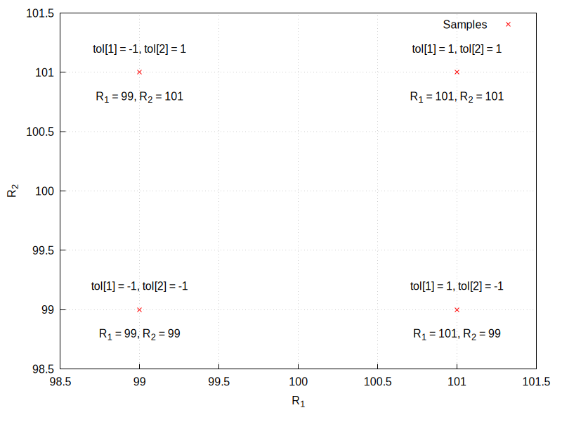
num=3 will cause the following combinations of tolerances to be tested:
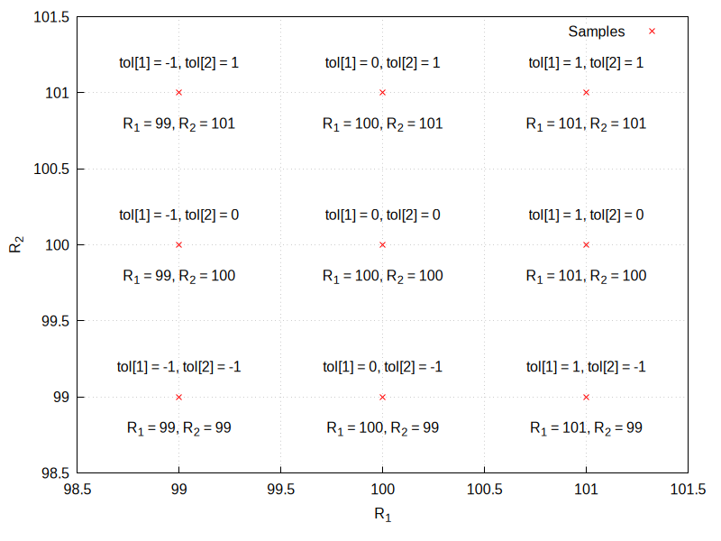
num=-500 will cause the following combinations of tolerances to
be tested, instead:
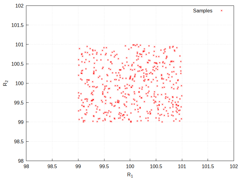
See also wc_defaultvaluespertol, wc_mintypmax,
wc_defaultvaluespertol,
wc_ewc_simplify and wc_005fmontecarlo.
Example:
maxima
(%i1) load("wrstcse")$
(%i2) vals: [
R_1= 1000.0*(1+tol[1]*.01),
R_2= 2000.0*(1+tol[2]*.01)
];
(%o2) [R_1 = 1000.0 (0.01 tol + 1),
1
R_2 = 2000.0 (0.01 tol + 1)]
2
(%i3) divider: U_Out=U_In*(R_1)/(R_1+R_2);
R_1 U_In
(%o3) U_Out = ---------
R_2 + R_1
(%i4) wc_systematic(subst(vals,rhs(divider)));
(%o4) [0.33333333333333337 U_In, 0.3311036789297659 U_In,
0.3289036544850498 U_In, 0.3355704697986577 U_In,
0.3333333333333333 U_In, 0.33112582781456956 U_In,
0.3377926421404682 U_In, 0.3355481727574751 U_In,
0.3333333333333333 U_In]
See also: wc_defaultvaluespertol, wc_mintypmax, wc_ewc_simplify, wc_montecarlo.
wc_tolappend (list1, list2, …) — Function
Appends lists of parameters from independent sources making sure that tolerances of all elements in one list will stay independent from all elements in the others.
Works like append() in that it appends all values from all of its arguments to make one big list. But this command, if one list happens to contain a tol[n] with the same n as another list, changes one of these n to a new value that makes it independent from all tolerances from the other list.
See also append.
Example:
maxima
(%i1) load("wrstcse")$
(%i2) val_a: [
R_1= 1000.0*(1+tol[1]*.01),
R_2= 1000.0*(1+tol[2]*.01)
];
(%o2) [R_1 = 1000.0 (0.01 tol + 1),
1
R_2 = 1000.0 (0.01 tol + 1)]
2
(%i3) val_b: [
R_3= 1000.0*(1+tol[1]*.01),
R_4= 1000.0*(1+tol[4]*.01)
];
(%o3) [R_3 = 1000.0 (0.01 tol + 1),
1
R_4 = 1000.0 (0.01 tol + 1)]
4
(%i4) append(val_a,val_b);
(%o4) [R_1 = 1000.0 (0.01 tol + 1),
1
R_2 = 1000.0 (0.01 tol + 1), R_3 = 1000.0 (0.01 tol + 1),
2 1
R_4 = 1000.0 (0.01 tol + 1)]
4
(%i5) wc_tolappend(val_a,val_b);
used = 1
(%o5) [R_1 = 1000.0 (0.01 tol + 1),
1
R_2 = 1000.0 (0.01 tol + 1), R_3 = 1000.0 (0.01 tol + 1),
2 5
R_4 = 1000.0 (0.01 tol + 1)]
4
See also: append.
wc_tolassumptions (expr) — Function
Adds the range of the tol[n] contained in expr to the assume database.
See also wc_inputvalueassumptions, wc_inputvalueranges and assume.
Example:
maxima
(%i1) load("wrstcse");
(%o1) /home/gunter/src/maxima-code/share/contrib/wrstcse.mac
(%i2) vals:[
R_1=100*(1+1/100*tol["R1"])*(1+1/100*tol["Temp"]),
R_2=200*(1+1/100*tol["R2"])*(1+1/100*tol["Temp"])];
tol tol
R1 Temp
(%o2) [R_1 = 100 (----- + 1) (------- + 1),
100 100
tol tol
R2 Temp
R_2 = 200 (----- + 1) (------- + 1)]
100 100
(%i3) float(wc_tolassumptions(%));
(%o3) [tol >= - 1.0, tol <= 1.0, tol >= - 1.0,
R1 R1 Temp
tol <= 1.0, tol >= - 1.0, tol <= 1.0]
Temp R2 R2
(%i4) is(tol[R_1]>tol[R_2]);
(%o4) unknown
(%i5) is(tol[R_1]>1);
(%o5) unknown
(%i6) is(tol[R_1]<-1);
(%o6) unknown
(%i7) is(tol[R_1]<0);
(%o7) unknown
(%i8) is(tol[R_2]>2);
(%o8) unknown
See also: wc_inputvalueassumptions, wc_inputvalueranges, assume.
wc_typicalvalues (expression) — Function
Returns what happens if all tol[n] happen to be 0, which moves all parameter to the middle of their tolerance range.
Example:
maxima
(%i1) load("wrstcse")$
(%i2) vals: [
R_1= 1000.0*(1+tol[1]*.01),
R_2= 2000.0*(1+tol[2]*.01)
];
(%o2) [R_1 = 1000.0 (0.01 tol + 1),
1
R_2 = 2000.0 (0.01 tol + 1)]
2
(%i3) divider:U_Out=U_In*R_1/(R_1+R_2);
R_1 U_In
(%o3) U_Out = ---------
R_2 + R_1
(%i4) wc_typicalvalues(vals);
(%o4) [R_1 = 1000.0, R_2 = 2000.0]
(%i5) wc_typicalvalues(subst(vals,divider));
(%o5) U_Out = 0.3333333333333333 U_In
Plotting
Plotting
adapt_depth — Variable
Default value: 5
The maximum number of splittings used by the adaptive plotting routine
of plot2d; integer must be a non-negative integer. A value
of zero means that adaptive plotting will not be used and the resulting
plot will have 1+4**nticks* points (see option nticks). To
have more control on the number of points and their positions, a list of
points can be created and then plotted using the discrete method
of plot2d.
See also: plot2d, nticks.
axes — Variable
Default value: true
Where symbol can be either true, false, x,
y or solid. If false, no axes are shown; if equal
to x or y only the x or y axis will be shown; if it is
equal to true, both axes will be shown and solid will show
the two axes with a solid line, rather than the default broken
line. This option does not have any effect in the 3 dimensional plots.
The single keywords axes and noaxes can be used as
synonyms for [axes, true] and [axes, false].
azimuth — Variable
Default value: 30
A plot3d plot can be thought of as starting with the x and y axis in the
horizontal and vertical axis, as in plot2d, and the z axis coming out of
the screen. The z axis is then rotated around the x axis through an
angle equal to elevation and then the new xy plane is rotated
around the new z axis through an angle azimuth. This option sets
the value for the azimuth, in degrees.
See also elevation.
See also: elevation, azimuth.
color — Variable
In 2d plots it defines the color (or colors) for the various curves. In
plot3d, it defines the colors used for the mesh lines of the
surfaces, when no palette is being used.
If there are more curves or surfaces than colors, the colors will be
repeated in sequence. The valid colors are red, green,
blue, magenta, cyan, yellow, orange,
violet, brown, gray, black, white, or
a string starting with the character # and followed by six hexadecimal
digits: two for the red component, two for green component and two for
the blue component. If the name of a given color is unknown color, black
will be used instead.
See also: plot3d.
color_bar — Variable
Default value: false in plot3d, true in mandelbrot and julia
Where symbol can be either true or false. If
true, whenever plot3d, mandelbrot or
julia use a palette to represent different values, a box will be
shown on the right, showing the corresponding between colors and values.
The single keywords color_bar and nocolor_bar can be used
as synonyms for [color_bar, true] and [color_bar, false].
See also: plot3d, mandelbrot, julia.
color_bar_tics — Variable
Defines the values at which a mark and a number will be placed in the
color bar. The first number is the initial value, the second the
increments and the third is the last value where a mark is placed. The
second and third numbers can be omitted. When only one number is given,
it will be used as the increment from an initial value that will be
chosen automatically. The single keyword color_bar_tics removes a
value given previously, making the graphic program use its default for
the values of the tics and nocolor_bar_tics will not show any
tics on the color bar.
elevation — Variable
Default value: 60
A plot3d plot can be thought of as starting with the x and y axis in the
horizontal and vertical axis, as in plot2d, and the z axis coming out of
the screen. The z axis is then rotated around the x axis through an
angle equal to elevation and then the new xy plane is rotated
around the new z axis through an angle azimuth. This option sets
the value for the elevation, in degrees.
See also azimuth.
See also: elevation, azimuth.
geomview — Variable
This is an abbreviation for [plot_format, geomview]. See
plot_005fformat.
See also: plot_format.
geomview_command — Variable
This variable stores the name of the command used to run the geomview
program when the plot format is geomview. Its default value is
“geomview”. If the geomview program is not found unless you give
its complete path or if you want to try a different version of it,
you may change the value of this variable. For instance,
maxima
(%i1) geomview_command: "/usr/local/bin/my_geomview"$
This variable must contain a string.
See also gnuplot_command and xmaxima_005fplot_005fcommand.
See also: gnuplot_command, xmaxima_plot_command.
get_plot_option (keyword, index) — Function
Returns the current default value of the option named keyword, which is a list. The optional argument index must be a positive integer which can be used to extract only one element from the list (element 1 is the name of the option).
See also set_plot_option, remove_plot_option and the
section on Plotting-Options.
See also: set_plot_option, remove_plot_option, Plotting-Options.
gnuplot — Variable
This is an abbreviation for [plot_format, gnuplot]. See
plot_005fformat.
See also: plot_format.
gnuplot_close () — Function
Closes the pipe to gnuplot which is used with the gnuplot_pipes format.
gnuplot_command — Variable
This variable stores the name of the command used to run the gnuplot
program when the plot format is gnuplot or
gnuplot_pipes. Its default value is “gnuplot”. If the gnuplot
program is not found unless you give its complete path or if you want to
try a different version of it, you may change the value of this
variable. For instance,
maxima
(%i1) gnuplot_command: "/usr/local/bin/my_gnuplot"$
This variable must contain a string.
See also geomview_command and xmaxima_005fplot_005fcommand.
See also: geomview_command, xmaxima_plot_command.
gnuplot_curve_styles — Variable
This is an obsolete option that has been replaced by style.
See also: style.
gnuplot_curve_titles — Variable
This is an obsolete option that has been replaced by legend described
above.
See also: legend.
gnuplot_default_term_command — Variable
[gnuplot_default_term_command, command]
The gnuplot command to set the terminal type for the default
terminal. It this option is not set, the command used will be: "set term wxt size 640,480 font \",12\"; set term pop".
gnuplot_dumb_term_command — Variable
[gnuplot_dumb_term_command, command]
The gnuplot command to set the terminal type for the dumb terminal. It
this option is not set, the command used will be: "set term dumb 79 22", which makes the text output 79 characters by 22 characters.
gnuplot_file_args — Variable
When a graphic file is going to be created using gnuplot, this
variable is used to specify the format used to print the file name given
to gnuplot. Its default value is “~a” in SBCL, Openmcl and GCL, and “~s”
in other lisp versions, which means that the name of the file will be
passed without quotes if SBCL, Openmcl or GCL are used, and within
quotes if other Lisp versions are used. The contents of this variable
can be changed in order to add options for the gnuplot program, adding
those options before the format directive “~s”.
gnuplot_out_file — Variable
It can be used to replace the default name for the file that contains
the commands that will interpreted by gnuplot, when the terminal is set
to default, or to replace the default name of the graphic file
that gnuplot creates, when the terminal is different from
default. If it contains one or more slashes, “/”, the name of
the file will be left as it is; otherwise, it will be appended to the
path of the temporary directory. The complete name of the files created
by the plotting commands is always sent as output of those commands so
they can be seen if the command is ended by semi-colon.
gnuplot_pdf_term_command — Variable
The gnuplot command to set the terminal type for the PDF
terminal. If this option is not set, the command used will be: "set term pdfcairo color solid lw 3 size 17.2 cm, 12.9 cm font \",18\"". See the gnuplot documentation for more information.
gnuplot_pipes — Variable
This is an abbreviation for [plot_format, gnuplot_pipes]. See
plot_005fformat.
See also: plot_format.
gnuplot_pm3d — Variable
With a value of false, it can be used to disable the use of PM3D
mode, which is enabled by default.
gnuplot_png_term_command — Variable
The gnuplot command to set the terminal type for the PNG terminal. If
this option is not set, the command used will be:
"set term pngcairo font \",12\"". See the gnuplot documentation
for more information.
gnuplot_postamble — Variable
This option inserts gnuplot commands after other commands sent to
Gnuplot and right before the plot command is sent. Any valid gnuplot
commands may be used. Multiple commands should be separated with a
semi-colon. See also gnuplot_005fpreamble.
See also: gnuplot_preamble.
gnuplot_preamble — Variable
This option inserts gnuplot commands before any other commands sent to
Gnuplot. Any valid gnuplot commands may be used. Multiple commands should
be separated with a semi-colon. See also gnuplot_005fpostamble.
See also: gnuplot_postamble.
gnuplot_ps_term_command — Variable
The gnuplot command to set the terminal type for the PostScript
terminal. If this option is not set, the command used will be: "set term postscript eps color solid lw 2 size 16.4 cm, 12.3 cm font \",24\"". See the gnuplot documentation for set term postscript for
more information.
gnuplot_replot () — Function
Updates the gnuplot window. If gnuplot_replot is called with a
gnuplot command in a string s, then s is sent to gnuplot
before reploting the window.
gnuplot_reset () — Function
Resets the state of gnuplot used with the gnuplot_pipes format. To
update the gnuplot window call gnuplot_replot after gnuplot_reset.
See also: gnuplot_replot.
gnuplot_restart () — Function
Closes the pipe to gnuplot which is used with the gnuplot_pipes
format and opens a new pipe.
gnuplot_script_file — Variable
Creates a plot with plot2d, plot3d, mandelbrot or
julia using the gnuplot plot_format and saving
the script sent to Gnuplot in the file specified by file_name_or_function.
The value file_name_or_function can be a string or a Maxima function of
one variable that returns a string. If that string corresponds to a
complete file path (directory and file name), the script will be created in
that file and will not be deleted after Maxima is closed; otherwise, the
string will give the name of a file to be created in the temporary directory
and deleted when Maxima is closed.
In this example, the script file name is set to “sin.gnuplot”, in the current directory.
maxima
(%i1) plot2d( sin(x), [x,0,2*%pi], [gnuplot_script_file, "./sin.gnuplot"]);
(%o1) [./sin.gnuplot]
In this example, gnuplot_prt(file) is a function that takes
the default file name, file. It constructs a full file name for
the data file by interpolating a random 8-digit integer with a pad of
zeros into the default file name (a 16-character random string followed
by “.gnuplot”). The temporary directory is determined by
maxima_tempdir (it is “/tmp” in this example).
maxima
(%i1) gnuplot_prt(file) := block([beg,end],
[beg,end] : split(file,"."),
printf(false,"~a_~8,'0d.~a",beg,random(10^8-1),end)) $
(%i2) plot2d( sin(x), [x,0,2*%pi], [gnuplot_script_file, gnuplot_prt]);
(%o2) [/tmp/nxuo4x28s6wocvjw_99211646.gnuplot]
By default, the script would have been saved in a file named
random-string.gnuplot (random-string = nxuo4x28s6wocvjw_99211646 in this
example) in the temporary directory. If the print statement in function
gnuplot_prt above included a directory path, the file would have
been saved in that directory rather than in the temporary directory.
See also: plot_format, maxima_tempdir.
gnuplot_send (s) — Function
Sends the command s to the gnuplot pipe. If that pipe is not currently opened, it will be opened before sending the command. s must be a string.
gnuplot_start () — Function
Opens the pipe to gnuplot used for plotting with the gnuplot_pipes
format. Is not necessary to manually open the pipe before plotting.
gnuplot_strings — Variable
With a value of true, all strings used in labels and titles will
be interpreted by gnuplot as “enhanced” text, if the terminal being used
supports it. In enhanced mode, some characters such as ^ and _ are not
printed, but interpreted as formatting characters. For a list of the
formatting characters and their meaning, see the documentation for enhanced
in Gnuplot. The default value for this option is false, which will
not treat any characters as formatting characters.
gnuplot_svg_background — Variable
[gnuplot_svg_background, color]
nognuplot_svg_background
Specify the background color for SVG image output.
color must be a string which specifies a color name recognized by Gnuplot,
or an RGB triple of the form "#xxxxxx" where x is a hexadecimal digit.
The default value is "white".
When the value of gnuplot_svg_background is false,
the background is the default determined by Gnuplot.
At present (April 2023),
the Gnuplot default is to specify the background in SVG output as "none".
nognuplot_svg_background, specified by itself without a value,
is equivalent to [gnuplot_svg_background, false].
gnuplot_svg_term_command — Variable
The gnuplot command to set the terminal type for the SVG
terminal. If this option is not set, the command used will be:
"set term svg font \",14\"". See the gnuplot documentation for
more information.
gnuplot_term — Variable
Sets the output terminal type for gnuplot. The argument terminal_name can be a string or one of the following 3 special symbols
default (default value)
Gnuplot output is displayed in a separate graphical window and the
gnuplot terminal used will be specified by the value of the option
gnuplot_005fdefault_005fterm_005fcommand.
dumb
Gnuplot output is saved to a file random-string.txt using “ASCII
art” approximation to graphics. If the option gnuplot_out_file is
set to filename, the plot will be saved there, instead of the
default random-string.gnuplot. The settings for the “dumb”
terminal of Gnuplot are given by the value of option
gnuplot_005fdumb_005fterm_005fcommand. If option run_viewer is set
to true and the plot_format is gnuplot that ASCII representation
will also be shown in the Maxima or Xmaxima console.
ps
Gnuplot generates commands in the PostScript page description language.
If the option gnuplot_out_file is set to filename, gnuplot
writes the PostScript commands to filename. Otherwise, it is
saved as maxplot.ps file. The settings for this terminal are given by the value of the option gnuplot_005fdumb_005fterm_005fcommand.
A string representing any valid gnuplot term specification
Gnuplot can generate output in many other graphical formats such as png,
jpeg, svg etc. To use those formats, option gnuplot_term can be
set to any supported gnuplot term name (which must be a symbol) or even a
full gnuplot term specification with any valid options (which must be a string). For
example [gnuplot_term, png] creates output in PNG (Portable
Network Graphics) format while [gnuplot_term, "png size 1000,1000"] creates PNG of 1000 x 1000 pixels size. If the option
gnuplot_out_file is set to filename, gnuplot writes the
output to filename. Otherwise, it is saved as
maxplot.term file, where term is gnuplot terminal
name.
See also: gnuplot_default_term_command, gnuplot_out_file, gnuplot_dumb_term_command, run_viewer.
gnuplot_view_args — Variable
This variable is the format used to parse the argument that will be
passed to the gnuplot program when the plot format is
gnuplot. Its default value is “-persist ~a” when SBCL, Openmcl or
GCL are used, and “-persist ~s” with other Lisp variants, where “~a” or
“~s” will be replaced with the name of the file where the gnuplot
commands have been written. The file name is usually
“random-string.gnuplot”; “~s” passes that name within quotes, while “~a”
passes it without quotes.
The option -persist tells gnuplot to exit after the commands in
the file have been executed, without closing the window that displays
the plot; even though the plot window remains it is inactive, namely,
some actions like trying to rotate a 3d plot or adding a grid will not
respond (the gnuplot_pipes format keeps the plot window active).
Those familiar with gnuplot, might want to change the value of this variable. For example, by changing it to:
maxima
(%i1) gnuplot_view_args: "~s -"$
gnuplot will not be closed after the commands in the file have been executed; thus, the window with the plot will remain active, as well as the gnuplot interactive shell where other commands can be issued in order to modify the plot (you may have to use ~a instead of ~s, depending on your Lisp version).
grid — Variable
Default value: 30, 30
Sets the number of grid points to use in the x- and y-directions for
three-dimensional plotting or for the julia and mandelbrot
programs.
For a way to actually draw a grid See grid2d.
See also: julia, mandelbrot, grid2d.
grid2d — Variable
Default value: false
Shows a grid of lines on the xy plane. The points where the grid lines
are placed are the same points where tics are marked in the x and y
axes, which can be controlled with the xtics and ytics
options. The single keywords grid2d and nogrid2d can be
used as synonyms for [grid2d, true] and [grid2d, false].
See also grid.
See also: xtics, ytics, grid.
iterations — Variable
Default value: 9
Number of iterations made by the programs mandelbrot and julia.
julia (x, y, …options…) — Function
Creates a graphic representation of the Julia set for the complex number
(x + i y). The two mandatory parameters x and y
must be real. This program is part of the additional package
dynamics, but that package does not have to be loaded; the first
time julia is used, it will be loaded automatically.
Each pixel in the grid is given a color corresponding to the number of
iterations it takes the sequence that starts at that point to move out
of the convergence circle of radius 2 centered at the origin. The number
of pixels in the grid is controlled by the grid plot option
(default 30 by 30). The maximum number of iterations is set with the
option iterations. The program sets its own default palette:
magenta, violet, blue, cyan, green, yellow, orange, red, brown and black,
but it can be changed by adding an explicit palette option in the
command.
The default domain used goes from -2 to 2 in both axes and can be
changed with the x and y options. By default, the two axes
are shown with the same scale, unless the option yx_ratio is used
or the option same_xy is disabled. Other general plot options are
also accepted.
The following example shows a region of the Julia set for the number
-0.55 + i0.6. The option color_bar_tics is used to prevent
Gnuplot from adjusting the color box up to 40, in which case the points
corresponding the maximum 36 iterations would not be black.
Warning: line 394 - example input lines must begin with ’
maxima
(%i1) julia (-0.55, 0.6, [iterations, 36], [x, -0.3, 0.2],
[y, 0.3, 0.9], [grid, 400, 400], [color_bar_tics, 0, 6, 36])$
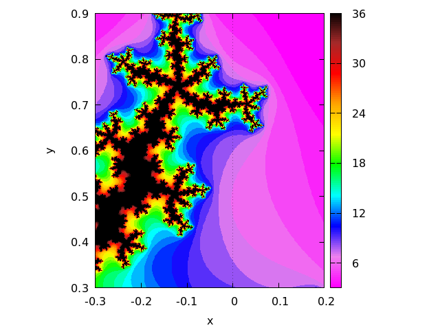
See also: grid, iterations, palette, yx_ratio, same_xy, color_bar_tics.
label — Variable
Writes one or several labels in the points with x, y coordinates indicated after each label.
legend — Variable
It specifies the labels for the plots when various plots are shown. If
there are more plots than the number of labels given, they will be
repeated. If given the value false, no legends will be shown.
By default, the names of the expressions or functions will be used, or
the words discrete1, discrete2, …, for discrete sets of points.
The single keyword legend removes any previously defined legends,
leaving it to the plotting program to set up a legend. The keyword
nolegend is a synonym for [legend, false].
levels — Variable
This option is used by plot2d to do contour plots. If only one
number is given after the keyword levels, it must be a natural
number; plot2d will try to plot that number of contours with
values between the minimum and maximum value of the expression given,
with the form d*10^n, where d is either 1, 2 or 5. Since not always it will
be possible to find that number of levels in that interval, the number of
contour lines show will be smaller than the number specified by this
option.
If more than one number are given after the keyword levels,
plot2d. will show the contour lines corresponding to those
values of the expression plotted, if they exist within the domain used.
See also: plot2d.
logx — Variable
Default value: false
Makes the horizontal axes to be scaled logarithmically. It can be either
true or false. The single keywords logx and nologx can be
used as synonyms for [logx, true] and [logx, false].
logy — Variable
Default value: false
Makes the vertical axes to be scaled logarithmically. It can be either
true or false.
The single keywords logy and nology can be used as
synonyms for [logy, true] and [logy, false].
make_transform ([var1, var2, var3], fx, fy, fz) — Function
Returns a function suitable to be used in the option transform_xy
of plot3d. The three variables var1, var2, var3 are
three dummy variable names, which represent the 3 variables given by the
plot3d command (first the two independent variables and then the
function that depends on those two variables). The three functions
fx, fy, fz must depend only on those 3 variables, and
will give the corresponding x, y and z coordinates that should be
plotted. There are two transformations defined by default:
polar_to_xy and spherical_005fto_005fxyz. See the documentation
for those two transformations.
See also: transform_xy, polar_to_xy, spherical_to_xyz.
mandelbrot (options) — Function
Creates a graphic representation of the Mandelbrot set. This program is
part of the additional package dynamics, but that package does
not have to be loaded; the first time mandelbrot is used, the package
will be loaded automatically.
This program can be called without any arguments, in which case it will
use a default value of 9 iterations per point, a grid with dimensions
set by the grid plot option (default 30 by 30) and a region
that extends from -2 to 2 in both axes. The options are all the same
that plot2d accepts, plus an option iterations to change the
number of iterations.
Each pixel in the grid is given a color corresponding to the number of
iterations it takes the sequence starting at zero to move out
of the convergence circle of radius 2, centered at the origin. The
maximum number of iterations is set by the option iterations.
The program uses its own default palette: magenta,violet, blue, cyan,
green, yellow, orange, red, brown and black, but it can be changed by
adding an explicit palette option in the command. By default, the
two axes are shown with the same scale, unless the option yx_ratio
is used or the option same_xy is disabled.
Example:
incorrect syntax: end of file while scanning expression.
^
maxima
(%i1) mandelbrot ([iterations,30], [x,-2,1], [y,-1.2,1.2], [grid,400,400])$
See also: grid, iterations, palette, yx_ratio, same_xy.
mesh_lines_color — Variable
Default value: black
It sets the color used by plot3d to draw the mesh lines, when a palette
is being used. It accepts the same colors as for the option
color (see the list of allowed colors in color). It
can also be given a value false to eliminate completely the mesh
lines. The single keyword mesh_lines_color removes any previously
defined colors, leaving it to the graphic program to decide what color
to use. The keyword nomesh_lines is a synonym for
[mesh_lines_color, false]
See also: color.
nticks — Variable
Default value: 29
When plotting functions with plot2d, it is gives the initial
number of points used by the adaptive plotting routine for plotting
functions. When plotting parametric functions with plot3d,
it sets the number of points that will be shown for the plot.
See also: plot2d, plot3d.
palette — Variable
It can consist of one palette or a list of several palettes. Each palette is a list with a keyword followed by values. If the keyword is gradient, it should be followed by a list of valid colors.
If the keyword is hue, saturation or value, it must be followed by 4 numbers. The first three numbers, which must be between 0 and 1, define the hue, saturation and value of a basic color to be assigned to the minimum value of z. The keyword specifies which of the three attributes (hue, saturation or value) will be increased according to the values of z. The last number indicates the increase corresponding to the maximum value of z. That last number can be bigger than 1 or negative; the corresponding values of the modified attribute will be rounded modulo 1.
Gnuplot only uses the first palette in the list; xmaxima will use the palettes in the list sequentially, when several surfaces are plotted together; if the number of palettes is exhausted, they will be repeated sequentially.
The color of the mesh lines will be given by the option
mesh_005flines_005fcolor. If palette is given the value
false, the surfaces will not be shaded but represented with a
mesh of curves only. In that case, the colors of the lines will be
determined by the option color.
The single keyword palette removes any palette previously
defined, leaving it to the graphic program to decide the palette to use
and nopalette is a synonym for [palette, false].
See also: mesh_lines_color, color.
pdf_file — Variable
Saves the plot into a PDF file with name equal to file_name,
rather than showing it in the screen. By default, the file will be
created in the directory defined by the variable
maxima_tempdir, unless file_name contains the character
“/”, in which case it will be assumed to contain the complete path where
the file should be created. The value of maxima_tempdir can be changed
to save the file in a different directory. When the option
gnuplot_pdf_term_command is also given, it will be used to set up
Gnuplot’s PDF terminal; otherwise, Gnuplot’s pdfcairo terminal
will be used with solid colored lines of width 3, plot
size of 17.2 cm by 12.9 cm and font of 18 points.
See also: maxima_tempdir, gnuplot_pdf_term_command.
plot2d (expr, range_x, options) — Function
There are 5 types of plots that can be plotted by plot2d:
- Explicit functions.
plot2d(expr, range_x, options), where expr is an expression that depends on only one variable, or the name of a function with one input parameter and numerical results. range_x is a list with three elements, the first one being the name of the variable that will be shown on the horizontal axis of the plot, and the other two elements should be two numbers, the first one smaller than the second, that define the minimum and maximum values to be shown on the horizontal axis. The name of the variable used in range_x must be the same variable on which expr depends. The result will show in the vertical axis the corresponding values of the expression or function for each value of the variable in the horizontal axis. - Implicit functions.
plot2d(expr_1=expr_2, range_x, range_y, options), where expr_1 and expr_2 are two expressions that can depend on one or two variables. range_x and range_y must be two lists of three elements that define the ranges for the variables in the two axes of the plot; the first element of each list is the name of the corresponding variable, and the other two elements are the minimum and maximum values for that variable. The two variables on which expr_1 and expr_2 can depend are those specified by range_x and range_y. The result will be a curve or a set of curves where the equation expr_1=expr_2 is true. - Parametric functions.
plot2d([parametric, expr_x, expr_y, range], options), where expr_x and expr_y are two expressions that depend on a single parameter. range must be a three-element list; the first element must be the name of the parameter on which expr_x and expr_y depend, and the other two elements must be the minimum and maximum values for that parameter. The result will be a curve in which the horizontal and vertical coordinates of each point are the values of expr_x and expr_y for a value of the parameter within the range given. - Set of points.
plot2d([discrete, points], options), displays a list of points, joined by segments by default. The horizontal and vertical coordinates of each of those points can be specified in three different ways: With two lists of the same length, in which the elements of the first list are the horizontal coordinates of the points and the second list are the vertical coordinates, or with a list of two-element lists, each one corresponding to the two coordinates of one of the points, or with a single list that defines the vertical coordinates of the points; in this last case, the horizontal coordinates of the n points will be assumed to be the first n natural numbers. - Contour lines.
plot2d([contour, expr], range_x, range_y, options), where expr is an expression that depends on two variables. range_x and range_y will be lists whose first elements are the names of those two variables, followed by two numbers that set the minimum and maximum values for them. The first variable will be represented along the horizontal axis and the second along the vertical axis. The result will be a set of curves along which the given expression has certain values. If those values are not specified with the optionlevels, plotd2d will try to choose, at the most, 8 values of the form d*10^n, where d is either 1, 2 or 5, all of them within the minimum and maximum values of expr within the given ranges.
At the end of a plot2d command several of the options described in
Plotting Options can be used. Many instances of the 5 types
described above can be combined into a single plot, by putting them
inside a list: plot2d ([type_1, …, type_n],
options). If one of the types included in the list require
range_x or range_y, those ranges should come immediately
after the list.
If there are several plots to be plotted, a legend will be
written to identity each of the expressions. The labels that should be
used in that legend can be given with the option legend. If that
option is not used, Maxima will create labels from the expressions or
function names.
Examples:
- Explicit function.
maxima
(%i1) plot2d (sin(x), [x, -%pi, %pi])$
 2. Implicit function.
maxima
(%i1) plot2d (x^2-y^3+3*y=2, [x,-2.5,2.5], [y,-2.5,2.5])$
 3. Parametric function.
maxima
(%i1) r: (exp(cos(t))-2*cos(4*t)-sin(t/12)^5)$
(%i2) plot2d([parametric, r*sin(t), r*cos(t), [t,-8*%pi,8*%pi]])$
 4. Set of points.
maxima
(%i1) plot2d ([discrete, makelist(i*%pi, i, 1, 5),
[0.6, 0.9, 0.2, 1.3, 1]])$
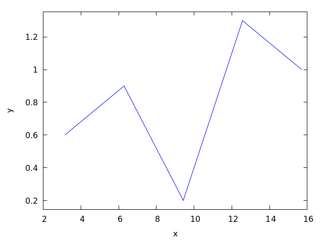 5. Contour lines.
maxima
(%i1) plot2d ([contour, u^3 + v^2], [u, -4, 4], [v, -4, 4])$
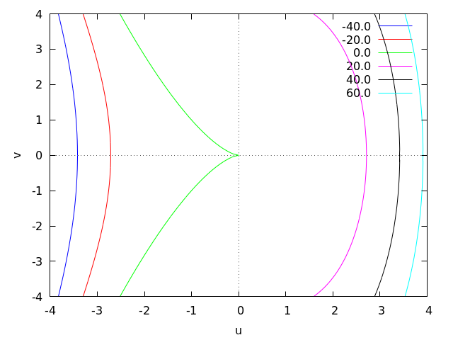
Examples using options.
If an explicit function grows too fast, the y option can be used
to limit the values in the vertical axis:
maxima
(%i1) plot2d (sec(x), [x, -2, 2], [y, -20, 20])$
plot2d: some values will be clipped.
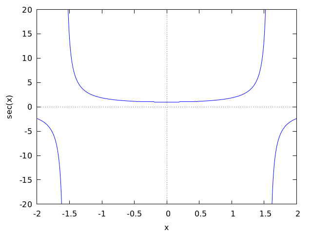
When the plot box is disabled, no labels are created for the axes. In
that case, instead of using xlabel and ylabel to set the
names of the axes, it is better to use option label, which
allows more flexibility. Option yx_ratio is used to change the
default rectangular shape of the plot; in this example the plot will
fill a square.
maxima
(%i1) plot2d ( x^2 - 1, [x, -3, 3], nobox, grid2d,
[yx_ratio, 1], [axes, solid], [xtics, -2, 4, 2],
[ytics, 2, 2, 6], [label, ["x", 2.9, -0.3],
["x^2-1", 0.1, 8]], [title, "A parabola"])$
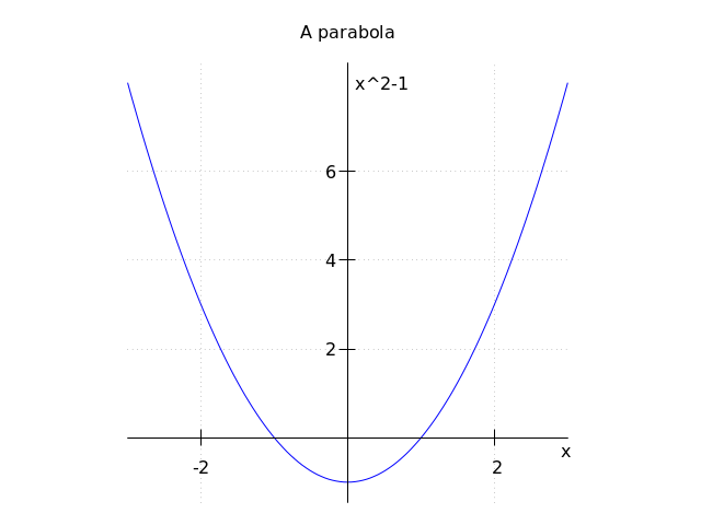
A plot with a logarithmic scale in the vertical axis:
maxima
(%i1) plot2d (exp(3*s), [s, -2, 2], logy)$
Plotting functions by name:
maxima
(%i1) F(x) := x^2 $
(%i2) :lisp (defun |$g| (x) (m* x x x))
$g
(%i2) H(x) := if x < 0 then x^4 - 1 else 1 - x^5 $
(%i3) plot2d ([F, G, H], [u, -1, 1], [y, -1.5, 1.5])$
Plot of a circumference of radius 1 centered at the origin, together with the
function y=-|x|. To prevent the circumference to look like an
ellipse, option same_xy is used to scale the two axes at the same
rate. Option nolegend is also used to remove the legend identifying
the two functions.
maxima
(%i1) plot2d([x^2+y^2=1, -abs(x)], [x, -1.5, 1.5], [y, -2, 2], same_xy,
nolegend);
(%o1) false
A plot of 200 random numbers between 0 and 9:
maxima
(%i1) plot2d ([discrete, makelist ( random(10), 200)])$
In the next example a table with three columns is saved in a file “data.txt” which is then read and the second and third column are plotted on the two axes:
maxima
(%i1) display2d:false$
(%i2) with_stdout ("data.txt", for x:0 thru 10 do
print (x, x^2, x^3))$
(%i3) data: read_matrix ("data.txt")$
(%i4) plot2d ([discrete, transpose(data)[2], transpose(data)[3]],
[style,points], [point_type,diamond], [color,red])$
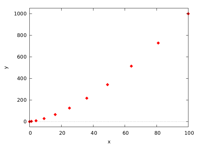
A plot of discrete data points together with a continuous function:
maxima
(%i1) xy: [[10, .6], [20, .9], [30, 1.1], [40, 1.3], [50, 1.4]]$
(%i2) plot2d([[discrete, xy], 2*%pi*sqrt(l/980)], [l,0,50],
[style, points, lines], [color, red, blue],
[point_type, asterisk],
[legend, "experiment", "theory"],
[xlabel, "pendulum's length (cm)"],
[ylabel, "period (s)"])$
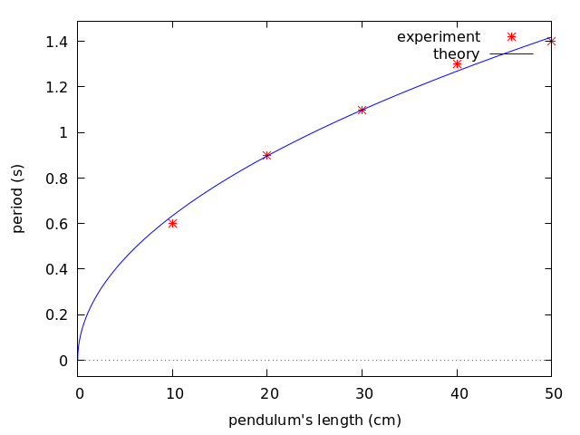
See also the Plotting Options section.
See also: Plotting-Options, legend, y, xlabel, ylabel, label, yx_ratio, same_xy, nolegend.
plot3d (expr, x_range, y_range, …, options, …) — Function
Displays a plot of one or more surfaces defined as functions of two variables or in parametric form.
The functions to be plotted may be specified as expressions or function names. The mouse can be used to rotate the plot looking at the surface from different sides.
Examples.
Plot of a function of two variables:
maxima
(%i1) plot3d (u^2 - v^2, [u, -2, 2], [v, -3, 3], [grid, 100, 100],
nomesh_lines)$
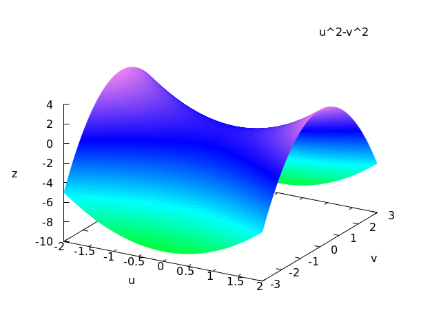
Use of the z option to limit a function that goes to infinity
(in this case the function is minus infinity on the x and y axes); this also
shows how to plot with only lines and no shading:
maxima
(%i1) plot3d ( log ( x^2*y^2 ), [x, -2, 2], [y, -2, 2], [z, -8, 4],
nopalette, [color, magenta])$
log: encountered log(0).
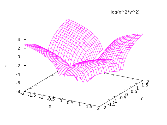
The infinite values of z can also be avoided by choosing a grid that does not fall on any points where the function is undefined, as in the next example, which also shows how to change the palette and how to include a color bar that relates colors to values of the z variable:
maxima
(%i1) plot3d (log (x^2*y^2), [x, -2, 2], [y, -2, 2],[grid, 29, 29],
[palette, [gradient, red, orange, yellow, green]],
color_bar, [xtics, 1], [ytics, 1], [ztics, 4],
[color_bar_tics, 4])$
log: encountered log(0).
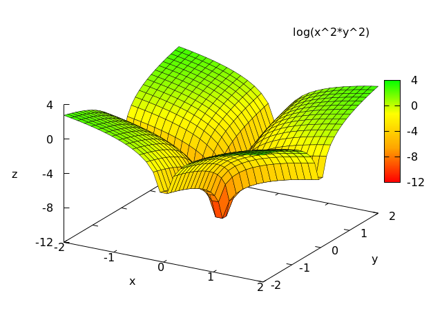
Two surfaces in the same plot. Ranges specific to one of the surfaces can be given by placing each expression and its ranges in a separate list; global ranges for the complete plot are also given after the function definitions.
maxima
(%i1) plot3d ([[-3*x - y, [x, -2, 2], [y, -2, 2]],
4*sin(3*(x^2 + y^2))/(x^2 + y^2), [x, -3, 3], [y, -3, 3]],
[x, -4, 4], [y, -4, 4])$
expt: undefined: 0 to a negative exponent.
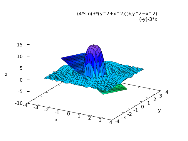
Plot of a Klein bottle, defined parametrically:
maxima
(%i1) expr_1: 5*cos(x)*(cos(x/2)*cos(y)+sin(x/2)*sin(2*y)+3)-10$
(%i2) expr_2: -5*sin(x)*(cos(x/2)*cos(y)+sin(x/2)*sin(2*y)+3)$
(%i3) expr_3: 5*(-sin(x/2)*cos(y)+cos(x/2)*sin(2*y))$
(%i4) plot3d ([expr_1, expr_2, expr_3], [x, -%pi, %pi],
[y, -%pi, %pi], [grid, 50, 50])$
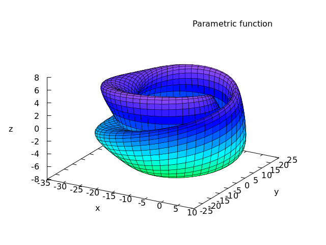
Plot of a “spherical harmonic” function, using the predefined
transformation, spherical_to_xyz to transform from spherical
coordinates to rectangular coordinates. See the documentation for
spherical_005fto_005fxyz.
maxima
(%i1) plot3d (sin(2*theta)*cos(phi), [theta,0,%pi], [phi,0,2*%pi],
[transform_xy, spherical_to_xyz], [grid, 30, 60], nolegend)$
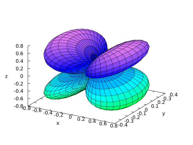
Use of the pre-defined function polar_to_xy to transform from
cylindrical to rectangular coordinates. See the documentation for
polar_005fto_005fxy.
maxima
(%i1) plot3d (r^.33*cos(th/3), [r,0,1], [th,0,6*%pi], nobox,
nolegend, [grid, 12, 80], [transform_xy, polar_to_xy])$
Plot of a sphere using the transformation from spherical to rectangular
coordinates. Option same_xyz is used to get the three axes
scaled in the same proportion. When transformations are used, it is not
convenient to eliminate the mesh lines, because Gnuplot will not show the
surface correctly.
maxima
(%i1) plot3d ( 5, [theta,0,%pi], [phi,0,2*%pi], same_xyz, nolegend,
[transform_xy, spherical_to_xyz], [mesh_lines_color,blue],
[palette,[gradient,"#1b1b4e", "#8c8cf8"]])$
Definition of a function of two-variables using a matrix. Notice the
single quote in the definition of the function, to prevent plot3d
from failing when it realizes that the matrix will require integer
indices.
maxima
(%i1) M: matrix([1,2,3,4], [1,2,3,2], [1,2,3,4], [1,2,3,3])$
(%i2) f(x, y) := float('M [round(x), round(y)])$
(%i3) plot3d (f(x,y), [x,1,4], [y,1,4], [grid,3,3], nolegend)$
By setting the elevation equal to zero, a surface can be seen as a map in which each color represents a different level.
maxima
(%i1) plot3d (cos (-x^2 + y^3/4), [x,-4,4], [y,-4,4], [zlabel,""],
[mesh_lines_color,false], [elevation,0], [azimuth,0],
color_bar, [grid,80,80], noztics, [color_bar_tics,1])$
See also Plotting-Options.
See also: z, spherical_to_xyz, polar_to_xy, same_xyz, Plotting-Options.
plot_format — Variable
Default value: gnuplot, in Windows systems, or gnuplot_pipes in
other systems.
Where format is one of the following: gnuplot, xmaxima,
gnuplot_pipes or geomview. The four possibilities: [plot_format, gnuplot], [plot_format, gnuplot_pipes], [plot_format, geomview] and [plot_format, xmaxima], can be abbreviated by the
keywords gnuplot, gnuplot_pipes, geomview and
xmaxima.
It sets the format to be used for plotting as explained in
Plotting-Formats.
See also: Plotting-Formats.
plot_options — Variable
This variable is being kept for compatibility with older versions of Wxmaxima,
but its use is deprecated. To set global plotting options, see their current
values or remove options, use set_plot_option,
get_plot_option remove_plot_option, and
reset_005fplot_005foptions.
See also: set_plot_option, get_plot_option, remove_plot_option, reset_plot_options.
plot_realpart — Variable
Default value: false
If set to true, the functions to be plotted will be considered as
complex functions whose real value should be plotted; this is equivalent
to plotting realpart(function). If set to false,
nothing will be plotted when the function does not give a real value.
For instance, when x is negative, log(x) gives a complex
value, with real value equal to log(abs(x)); if
plot_realpart were true, log(-5) would be plotted
as log(5), while nothing would be plotted if plot_realpart
were false. The single keyword plot_realpart can be used
as a synonym for [plot_realpart, true] and noplot_realpart
is a synonym for [plot_realpart, false].
plotepsilon — Variable
Default value: 1e-6
This value is used by plot2d when plotting implicit functions or
contour lines. When plotting an explicit function expr_1=expr_2,
it is converted into expr_1-expr_2 and the points where that equals
zero are searched. When a contour line for expr equal to some value
is going to be plotted, the points where expr minus that value
are equal to zero are searched. The search is done by computing those
expressions at a grid of points (see sample). If at one of the
points in that grid the absolute value of the expression is less than
the value of plotepsilon, it will be assumed to be zero, and
therefore, as being part of the curve to be plotted.
See also: plot2d, sample.
png_file — Variable
Saves the plot into a PNG graphics file with name equal to file_name,
rather than showing it in the screen. By default, the file will be
created in the directory defined by the variable
maxima_tempdir, unless file_name contains the character
“/”, in which case it will be assumed to contain the complete path where
the file should be created. The value of maxima_tempdir can be changed
to save the file in a different directory. When the option
gnuplot_png_term_command is also given, it will be used to set up
Gnuplot’s PNG terminal; otherwise, Gnuplot’s pngcairo terminal
will be used, with a font of size 12.
See also: maxima_tempdir, gnuplot_png_term_command.
point_type — Variable
In gnuplot, each set of points to be plotted with the style “points”
or “linespoints” will be represented with objects taken from this
list, in sequential order. If there are more sets of points than objects
in this list, they will be repeated sequentially.
The possible objects that can be used are: bullet, circle,
plus, times, asterisk, box, square,
triangle, delta, wedge, nabla, diamond,
lozenge.
Function: polar_to_xy
It can be given as value for the transform_xy option of
plot3d. Its effect will be to interpret the two independent variables in
plot3d as the distance from the z axis and the azimuthal angle (polar
coordinates), and transform them into x and y coordinates.
See also: transform_xy.
ps_file — Variable
Saves the plot into a Postscript file with name equal to file_name,
rather than showing it in the screen. By default, the file will be
created in the directory defined by the variable
maxima_tempdir, unless file_name contains the character
“/”, in which case it will be assumed to contain the complete path where
the file should be created. The value of maxima_tempdir can be changed
to save the file in a different directory. When the option
gnuplot_ps_term_command is also given, it will be used to set up
Gnuplot’s Postscript terminal; otherwise, Gnuplot’s postscript terminal
will be used with the EPS option, solid colored lines of width 2, plot
size of 16.4 cm by 12.3 cm and font of 24 points.
See also: maxima_tempdir, gnuplot_ps_term_command.
remove_plot_option (name) — Function
Removes the global value of an option. The name of the option must be given.
See also set_plot_option, get_plot_option and
Plotting Options.
See also: set_plot_option, get_plot_option, Plotting-Options.
reset_plot_options () — Function
Sets the default global values of the plotting options. After changing the global values of some plotting options, this function is used to recovered the same values as when Maxima was started.
run_viewer — Variable
Default value: true
This option is only used when the plot format is gnuplot and the
terminal is default or when the Gnuplot terminal is set to
dumb (see gnuplot_term) and can have a true or false
value.
If the terminal is default, a file random-string.gnuplot (or
other name specified with gnuplot_out_file) is created with the
gnuplot commands necessary to generate the plot. Option run_viewer
controls whether or not Gnuplot will be launched to execute those
commands and show the plot.
If the terminal is default, gnuplot is run to execute the
commands in random-string.gnuplot, producing another file
maxplot.txt (or other name specified with
gnuplot_out_file). Option run_viewer controls whether or
not that file, with an ASCII representation of the plot, will be shown
in the Maxima or Xmaxima console.
Its default value, true, makes the plots appear in either the console or
a separate graphics window. run_viewer and norun_viewer
are synonyms for [run_viewer, true] and [run_viewer, false].
See also: gnuplot_term, gnuplot_out_file.
same_xy — Variable
It can be either true or false. If true, the scales used in the x and y
axes will be the same, in either 2d or 3d plots. See also
yx_005fratio. same_xy and nosame_xy are synonyms for
[same_xy, true] and [same_xy, false].
See also: yx_ratio.
same_xyz — Variable
It can be either true or false. If true, the scales used in the 3 axes
of a 3d plot will be the same. same_xyz and nosame_xyz are
synonyms for [same_xyz, true] and [same_xyz, false].
sample — Variable
Default value: [sample, 47, 47]
nx and ny must be two natural numbers that will be used by
plot2d to look for the points that make part of the plot of an
implicit function or a contour line. The domain is divided into nx
intervals in the horizontal axis and ny intervals in the vertical
axis and the numerical value of the expression is computed at the
borders of those intervals. Higher values of nx and ny will
give smoother curves, but will increase the time needed to trace the
plot. When there are critical points in the plot where the curve changes
direction, to get better results it is more important to try to make
those points to be at the border of the intervals, rather than
increasing nx and ny.
See also: plot2d.
set_plot_option (option) — Function
Accepts any of the options listed in the section Plotting Options,
and saves them for use in plotting commands. The values of the options set
in each plotting command will have precedence, but if those options are
not given, the default values set with this function will be used.
set_plot_option evaluates its argument and returns the complete
list of options (after modifying the option given). If called without
any arguments, it will simply show the list of current default options.
See also remove_plot_option, get_plot_option and the section
on Plotting-Options.
Example:
Modification of the grid values.
maxima
(%i1) set_plot_option ([grid, 30, 40]);
(%o1) [[plot_format, gnuplot_pipes], [grid, 30, 40],
[run_viewer, true], [axes, true], [nticks, 29],
[adapt_depth, 5], [color, blue, red, green, magenta, black,
cyan], [point_type, bullet, box, triangle, plus, times,
asterisk], [palette, [hue, 0.33333333, 0.7, 1, 0.5],
[hue, 0.8, 0.7, 1, 0.4]], [gnuplot_svg_background, white],
[gnuplot_preamble, ], [gnuplot_term, default]]
See also: Plotting-Options, remove_plot_option, get_plot_option, grid.
Function: spherical_to_xyz
It can be given as value for the transform_xy option of
plot3d. Its effect will be to interpret the two independent
variables and the function in plot3d as the spherical coordinates
of a point (first, the angle with the z axis, then the angle of the xy
projection with the x axis and finally the distance from the origin) and
transform them into x, y and z coordinates.
See also: transform_xy, plot3d.
style — Variable
The styles that will be used for the various functions or sets of data in a 2d plot. The word style must be followed by one or more styles. If there are more functions and data sets than the styles given, the styles will be repeated. Each style can be either lines for line segments, points for isolated points, linespoints for segments and points, or dots for small isolated dots. Gnuplot accepts also an impulses style.
Each of the styles can be enclosed inside a list with some additional parameters. lines accepts one or two numbers: the width of the line and an integer that identifies a color. The default color codes are: 1: blue, 2: red, 3: magenta, 4: orange, 5: brown, 6: lime and 7: aqua. If you use Gnuplot with a terminal different than X11, those colors might be different; for example, if you use the option [gnuplot_term, ps], color index 4 will correspond to black, instead of orange.
points accepts one, two, or three parameters; the first parameter is the radius of the points, the second parameter is an integer that selects the color, using the same code used for lines and the third parameter is currently used only by Gnuplot and it corresponds to several objects instead of points. The default types of objects are: 1: filled circles, 2: open circles, 3: plus signs, 4: x, 5: *, 6: filled squares, 7: open squares, 8: filled triangles, 9: open triangles, 10: filled inverted triangles, 11: open inverted triangles, 12: filled lozenges and 13: open lozenges.
linespoints accepts up to five parameters: line width, points radius, color, type of object to replace the points, and the gnuplot pointinterval option to control space between points.
See also color and point_005ftype.
See also: color, point_type.
svg_file — Variable
Saves the plot into an SVG file with name equal to file_name,
rather than showing it in the screen. By default, the file will be
created in the directory defined by the variable
maxima_tempdir, unless file_name contains the character
“/”, in which case it will be assumed to contain the complete path where
the file should be created. The value of maxima_tempdir can be changed
to save the file in a different directory. When the option
gnuplot_svg_term_command is also given, it will be used to set up
Gnuplot’s SVG terminal; otherwise, Gnuplot’s svg terminal
will be used with font of 14 points.
See also: maxima_tempdir, gnuplot_svg_term_command.
t — Variable
Default range for parametric plots.
title — Variable
Defines a title that will be written at the top of the plot.
transform_xy — Variable
Where symbol is either false or the result obtained by
using the function transform_xy. If different from false,
it will be used to transform the 3 coordinates in
plot3d. notransform_xy removes any transformation function
previously defined.
See make_transform, polar_to_xy and
spherical_005fto_005fxyz.
See also: make_transform, polar_to_xy, spherical_to_xyz.
window — Variable
Opens the plot in window number n, instead of the default window 0. If window number n is already opened, the plot in that window will be replaced by the current plot.
x — Variable
When used as the first option in a plot2d command (or any of the
first two in plot3d), it indicates that the first independent variable
is x and it sets its range. It can also be used again after the first
option (or after the second option in plot3d) to define the effective
horizontal domain that will be shown in the plot.
See also: plot2d, plot3d.
xlabel — Variable
Specifies the string that will label the first axis; if this
option is not used, that label will be the name of the independent
variable, when plotting functions with plot2d the name of the
first variable, when plotting surfaces with plot3d, or the first
expression in the case of a parametric plot. noxlabel is equivalent
to [xlabel, ""], which does not print any label on the first axis.
See also: plot2d, plot3d.
xmaxima — Variable
This is an abbreviation for [plot_format, xmaxima]. See
plot_005fformat.
See also: plot_format.
xmaxima_plot_command — Variable
This variable stores the name of the command used to run the xmaxima
program when the plot format is xmaxima.
Its default value is “xmaxima”. If the xmaxima
program is not found unless you give its complete path or if you want to
try a different version of it, you may change the value of this
variable. For instance,
maxima
(%i1) xmaxima_plot_command: "/usr/local/bin/my_xmaxima"$
This variable must contain a string.
See also gnuplot_command and geomview_005fcommand.
See also: gnuplot_command, geomview_command.
xtics — Variable
Defines the values at which a mark and a number will be placed in the x
axis. The first number is the initial value, the second the increments
and the third is the last value where a mark is placed. The second and
third numbers can be omitted, in which case the first number is the
increment from an initial value that will be chosen by the graphic
program. If [xtics, false] is used, no marks or numbers will be
shown along the x axis.
The single keyword xtics removes any values previously
defined, leaving it to the graphic program to decide the values to use
and noxtics is a synonym for [xtics, false]
xy_scale — Variable
In a 2d plot, it defines the ratio of the total size of the Window to the size that will be used for the plot. The two numbers given as arguments are the scale factors for the x and y axes.
This option does not change the size of the graphic window or the placement
of the graph in the window. If you want to change the aspect ratio of the
plot, it is better to use option yx_005fratio. For instance,
[yx_ratio, 10] instead of [xy_scale, 0.1, 1].
See also: yx_ratio.
y — Variable
When used as one of the first two options in plot3d, it indicates
that one of the independent variables is y and it sets its range. Otherwise,
it defines the effective domain of the second variable that will be
shown in the plot.
See also: plot3d.
ylabel — Variable
Specifies the string that will label the second axis; if this
option is not used, that label will be “y”, when plotting explicit
functions with plot2d, or the name of the second variable, when
plotting surfaces with plot3d, or the second expression in the
case of a parametric plot. noylabel is equivalent to
[ylabel, ""], which does not print any label on the second axis.
See also: plot2d, plot3d.
ytics — Variable
Defines the values at which a mark and a number will be placed in the y
axis. The first number is the initial value, the second the increments
and the third is the last value where a mark is placed. The second and
third numbers can be omitted, in which case the first number is the
increment from an initial value that will be chosen by the graphic
program. If [ytics, false] is used, no marks or numbers will be
shown along the y axis.
The single keyword ytics removes any values previously
defined, leaving it to the graphic program to decide the values to use
and noytics is a synonym for [ytics, false]
yx_ratio — Variable
In a 2d plot, the ratio between the vertical and the horizontal sides of
the rectangle used to make the plot. See also same_005fxy.
See also: same_xy.
z — Variable
Used in plot3d to set the effective range of values of z that will be
shown in the plot.
See also: plot3d.
zlabel — Variable
Specifies the string that will label the third axis, when using
plot3d. If this option is not used, that label will be “z”,
when plotting surfaces, or the third expression in the case of a
parametric plot. It can not be used with set_plot_option and it
will be ignored by plot2d. nozlabel is equivalent to
[zlabel, ""], which does not print any label on the third axis.
See also: plot3d, set_plot_option, plot2d.
zmin — Variable
In 3d plots, the value of z that will be at the bottom of the plot box.
The single keyword zmin removes any value previously
defined, leaving it to the graphic program to decide the value to use.
ztics — Variable
Defines the values at which a mark and a number will be placed in the z
axis. The first number is the initial value, the second the increments
and the third is the last value where a mark is placed. The second and
third numbers can be omitted, in which case the first number is the
increment from an initial value that will be chosen by the graphic
program. If [ztics, false] is used, no marks or numbers will be
shown along the z axis.
The single keyword ztics removes any values previously
defined, leaving it to the graphic program to decide the values to use
and noztics is a synonym for [ztics, false]
descriptive
barsplot (data1, data2, …, option_1, option_2, …) — Function
Plots bars diagrams for discrete statistical variables, both for one or multiple samples.
data can be a list of outcomes representing one sample, or a matrix of m rows and n columns, representing n samples of size m each.
Available options are:
box_width (default, 3/4): relative width of rectangles. This
value must be in the range [0,1].
grouping (default, clustered): indicates how multiple samples are
shown. Valid values are: clustered and stacked.
groups_gap (default, 1): a positive integer number representing
the gap between two consecutive groups of bars.
bars_colors (default, []): a list of colors for multiple samples.
When there are more samples than specified colors, the extra necessary colors
are chosen at random. See color to learn more about them.
frequency (default, absolute): indicates the scale of the
ordinates. Possible values are: absolute, relative,
and percent.
ordering (default, orderlessp): possible values are orderlessp or ordergreatp,
indicating how statistical outcomes should be ordered on the x-axis.
sample_keys (default, []): a list with the strings to be used in the legend.
When the list length is other than 0 or the number of samples, an error message is returned.
start_at (default, 0): indicates where the plot begins to be plotted on the
x axis.
All global draw options, except xtics, which is
internally assigned by barsplot.
If you want to set your own values for this option or want to build
complex scenes, make use of barsplot_description. See example below.
The following local Package-draw options: key, color_draw,
fill_color, fill_density and line_005fwidth.
See also
barsplot.
There is also a function wxbarsplot for creating embedded
histograms in interfaces wxMaxima and iMaxima. barsplot in a
multiplot context.
Examples:
Univariate sample in matrix form. Absolute frequencies.
(%i1) load ("descriptive")$
(%i2) m : read_matrix (file_search ("biomed.data"))$
(%i3) barsplot(
col(m,2),
title = "Ages",
xlabel = "years",
box_width = 1/2,
fill_density = 3/4)$
Two samples of different sizes, with relative frequencies and user declared colors.
(%i1) load ("descriptive")$
(%i2) l1:makelist(random(10),k,1,50)$
(%i3) l2:makelist(random(10),k,1,100)$
(%i4) barsplot(
l1,l2,
box_width = 1,
fill_density = 1,
bars_colors = [black, grey],
frequency = relative,
sample_keys = ["A", "B"])$
Four non numeric samples of equal size.
(%i1) load ("descriptive")$
(%i2) barsplot(
makelist([Yes, No, Maybe][random(3)+1],k,1,50),
makelist([Yes, No, Maybe][random(3)+1],k,1,50),
makelist([Yes, No, Maybe][random(3)+1],k,1,50),
makelist([Yes, No, Maybe][random(3)+1],k,1,50),
title = "Asking for something to four groups",
ylabel = "# of individuals",
groups_gap = 3,
fill_density = 0.5,
ordering = ordergreatp)$
Stacked bars.
(%i1) load ("descriptive")$
(%i2) barsplot(
makelist([Yes, No, Maybe][random(3)+1],k,1,50),
makelist([Yes, No, Maybe][random(3)+1],k,1,50),
makelist([Yes, No, Maybe][random(3)+1],k,1,50),
makelist([Yes, No, Maybe][random(3)+1],k,1,50),
title = "Asking for something to four groups",
ylabel = "# of individuals",
grouping = stacked,
fill_density = 0.5,
ordering = ordergreatp)$
For bars diagrams related options, see barsplot of package Package-draw
See also functions histogram and piechart.
See also: Package-draw, key, color_draw, fill_color, fill_density, line_width, barsplot, histogram, piechart.
barsplot_description (…) — Function
Function barsplot_description creates a graphic object
suitable for creating complex scenes, together with other
graphic objects.
Example: barsplot in a multiplot context.
(%i1) load ("descriptive")$
(%i2) l1:makelist(random(10),k,1,50)$
(%i3) l2:makelist(random(10),k,1,100)$
(%i4) bp1 :
barsplot_description(
l1,
box_width = 1,
fill_density = 0.5,
bars_colors = [blue],
frequency = relative)$
(%i5) bp2 :
barsplot_description(
l2,
box_width = 1,
fill_density = 0.5,
bars_colors = [red],
frequency = relative)$
(%i6) draw(gr2d(bp1), gr2d(bp2))$
boxplot (data) — Function
This function plots box-and-whisker diagrams. Argument data can be a list,
which is not of great interest, since these diagrams are mainly used for
comparing different samples, or a matrix, so it is possible to compare
two or more components of a multivariate statistical variable.
But it is also allowed data to be a list of samples with
possible different sample sizes, in fact this is the only function
in package descriptive that admits this type of data structure.
The box is plotted from the first quartile to the third, with an horizontal
segment situated at the second quartile or median. By default, lower and
upper whiskers are plotted at the minimum and maximum values,
respectively. Option range can be used to indicate that values greater
than quantile(x,3/4)+range*(quantile(x,3/4)-quantile(x,1/4)) or
less than quantile(x,1/4)-range*(quantile(x,3/4)-quantile(x,1/4))
must be considered as outliers, in which case they are plotted as
isolated points, and the whiskers are located at the extremes of the rest of
the sample.
Available options are:
box_width (default, 3/4): relative width of boxes.
This value must be in the range [0,1].
box_orientation (default, vertical): possible values: vertical
and horizontal.
range (default, inf): positive coefficient of the interquartilic range
to set outliers boundaries.
outliers_size (default, 1): circle size for isolated outliers.
All draw options, except points_joined, point_size, point_type,
xtics, ytics, xrange, and yrange, which are
internally assigned by boxplot.
If you want to set your own values for this options or want to build
complex scenes, make use of boxplot_description.
The following local draw options: key, color,
and line_width.
There is also a function wxboxplot for creating embedded
histograms in interfaces wxMaxima and iMaxima.
Examples:
Box-and-whisker diagram from a multivariate sample.
(%i1) load ("descriptive")$
(%i2) s2 : read_matrix(file_search("wind.data"))$
(%i3) boxplot(s2,
box_width = 0.2,
title = "Windspeed in knots",
xlabel = "Stations",
color = red,
line_width = 2)$
Box-and-whisker diagram from three samples of different sizes.
(%i1) load ("descriptive")$
(%i2) A :
[[6, 4, 6, 2, 4, 8, 6, 4, 6, 4, 3, 2],
[8, 10, 7, 9, 12, 8, 10],
[16, 13, 17, 12, 11, 18, 13, 18, 14, 12]]$
(%i3) boxplot (A, box_orientation = horizontal)$
Option range can be used to handle outliers.
(%i1) load ("descriptive")$
B: [[7, 15, 5, 8, 6, 5, 7, 3, 1],
[10, 8, 12, 8, 11, 9, 20],
[23, 17, 19, 7, 22, 19]] $
boxplot (B, range=1)$
boxplot (B, range=1.5, box_orientation = horizontal)$
draw2d(
boxplot_description(
B,
range = 1.5,
line_width = 3,
outliers_size = 2,
color = red,
background_color = light_gray),
xtics = {["Low",1],["Medium",2],["High",3]}) $
boxplot_description (…) — Function
Function boxplot_description creates a graphic object
suitable for creating complex scenes, together with other
graphic objects.
histogram (list) — Function
Constructs and displays a histogram from a data sample. Data must be stored as a list of numbers, or a matrix of one row or one column.
Optional arguments:
nclasses (default, 10):
the number of classes (also called bins) in the histogram,
or a list of two numbers (the least and greatest values included in the histogram),
or a list of three numbers (the least and greatest values included in the histogram, and the number of classes),
or a set containing the endpoints of the class intervals,
or a symbol specifying the name of one of three algorithms to automatically determine the number of classes:
fd (Ref. [1]), scott (Ref. [2]), or sturges (Ref. [3]).
A class interval excludes its left endpoint and includes its right endpoint, except for the first interval, which includes both the left and right endpoints. It is assumed that class intervals are contiguous. That is, the right endpoint of one interval is equal to the left endpoint of the next.
frequency (default, absolute): indicates the scale of the vertical axis.
Possible values are: absolute (heights of bars add up to number of data),
relative (heights of bars add up to 1),
percent (heights of bars add up to 100),
and density (total area of histogram is 1).
htics (default, auto): format of tic marks on the horizontal axis.
Possible values are: auto (tics are placed automatically),
endpoints (tics are placed at the divisions between classes),
intervals (classes are labeled with the corresponding intervals),
or a list of labels, one for each class.
All global draw options, except xrange, yrange,
and xtics, which are internally assigned by histogram.
If you want to set your own values for these options, make use of
histogram_description.
The following local Package-draw options: key,
fill_color, fill_density, and line_005fwidth.
Note that the outlines of bars,
as well as the interior of bars when fill_density is nonzero,
are drawn with fill_color, not color.
histogram honors the global option histogram_skyline.
When histogram_skyline is true,
histogram and histogram_description construct “skyline” plots,
which shows the outline of the histogram bars,
instead of drawing all the vertical segments.
Otherwise (the default), histograms are displayed with bars showing vertical segments.
There is also a function wxhistogram for creating embedded
histograms in interfaces wxMaxima and iMaxima.
See also continuous_freq,
which, like histogram,
counts data in intervals,
but returns the counts instead of displaying a graphic representation.
See also barsplot.
Examples:
A simple histogram with eight classes:
(%i1) load ("descriptive")$
(%i2) s1 : read_list (file_search ("pidigits.data"))$
(%i3) histogram (
s1,
nclasses = 8,
title = "pi digits",
xlabel = "digits",
ylabel = "Absolute frequency",
fill_color = grey,
fill_density = 0.6)$
Setting the limits of the histogram to -2 and 12, with 3 classes. Also, we introduce predefined tics:
(%i1) load ("descriptive")$
(%i2) s1 : read_list (file_search ("pidigits.data"))$
(%i3) histogram (
s1,
nclasses = [-2,12,3],
htics = ["A", "B", "C"],
terminal = png,
fill_color = "#23afa0",
fill_density = 0.6)$
Bounds for varying class widths.
(%i1) load ("descriptive")$
(%i2) s1 : read_list (file_search ("pidigits.data"))$
(%i3) histogram (s1, nclasses = {0,3,6,7,11})$
Freedman-Diaconis formula for the number of classes.
(%i1) load ("descriptive")$
(%i2) s1 : read_list (file_search ("pidigits.data"))$
(%i3) histogram(s1, nclasses=fd) $
References:
[1] Freedman, D., and Diaconis, P. (1981) On the histogram as a density estimator: L_2 theory. Zeitschrift fur Wahrscheinlichkeitstheorie und verwandte Gebiete 57, 453-476.
[2] Scott, D. W. (1979) On optimal and data-based histograms. Biometrika 66, 605-610.
[3] Sturges, H. A. (1926) The choice of a class interval. Journal of the American Statistical Association 21, 65-66.
See also: Package-draw, key, fill_color, fill_density, line_width, continuous_freq, barsplot.
histogram_description (…) — Function
Creates a graphic object which represents a histogram.
Such an object is suitable for creating complex scenes together with other graphic objects,
to be displayed by draw2d.
histogram_description takes the same arguments
as the stand-alone function histogram.
See histogram for more information.
Example:
We make use of histogram_description for setting
xrange and adding an explicit curve into the scene:
(%i1) load ("descriptive")$
(%i2) ( load("distrib"),
m: 14, s: 2,
s2: random_normal(m, s, 1000) ) $
(%i3) draw2d(
grid = true,
xrange = [5, 25],
histogram_description(
s2,
nclasses = 9,
frequency = density,
fill_density = 0.5),
explicit(pdf_normal(x,m,s), x, m - 3*s, m + 3* s))$
See also: histogram.
histogram_skyline — Variable
Default value: false
When histogram_skyline is true,
histogram and histogram_description construct “skyline” plots,
which shows the outline of the histogram bars,
instead of drawing all the vertical segments.
The outline is drawn with the current fill_color (not the current color).
The interior of the histogram is filled with fill_color,
but only if fill_density is nonzero.
Otherwise, histograms are displayed with bars showing vertical segments.
Examples:
Construct a skyline histogram, and an ordinary histogram for comparison, on the same plot.
(%i1) load ("descriptive") $
(%i2) L: read_list (file_search ("pidigits.data")) $
(%i3) histogram_skyline: true $
(%i4) skyline_hist: histogram_description (L) $
(%i5) histogram_skyline: false $
(%i6) ordinary_hist: histogram_description (L) $
(%i7) draw (gr2d (skyline_hist), gr2d (ordinary_hist)) $
Continuing the preceding example.
Set display options for fill_color and fill_density.
(%i8) histogram_skyline: true $
(%i9) skyline_hist: histogram_description (L, fill_color = blue, fill_density = 0.2) $
(%i10) histogram_skyline: false $
(%i11) ordinary_hist: histogram_description (L, fill_color = blue, fill_density = 0.2) $
(%i12) draw (gr2d (skyline_hist), gr2d (ordinary_hist)) $
piechart (list) — Function
Similar to barsplot, but plots sectors instead of rectangles.
Available options are:
sector_colors (default, []): a list of colors for sectors.
When there are more sectors than specified colors, the extra necessary colors
are chosen at random. See color to learn more about them.
pie_center (default, [0,0]): diagram’s center.
pie_radius (default, 1): diagram’s radius.
All global draw options, except key, which is
internally assigned by piechart.
If you want to set your own values for this option or want to build
complex scenes, make use of piechart_description.
The following local draw options: key, color,
fill_density and line_width. See also
ellipse
There is also a function wxpiechart for
creating embedded histograms in interfaces wxMaxima and iMaxima.
Example:
(%i1) load ("descriptive")$
(%i2) s1 : read_list (file_search ("pidigits.data"))$
(%i3) piechart(
s1,
xrange = [-1.1, 1.3],
yrange = [-1.1, 1.1],
title = "Digit frequencies in pi")$
See also function barsplot.
See also: barsplot.
piechart_description (…) — Function
Function piechart_description creates a graphic object
suitable for creating complex scenes, together with other
graphic objects.
scatterplot (list) — Function
Plots scatter diagrams both for univariate (list) and multivariate (matrix) samples.
Available options are the same admitted by histogram.
There is also a function wxscatterplot for
creating embedded histograms in interfaces wxMaxima and iMaxima.
Examples:
Univariate scatter diagram from a simulated Gaussian sample.
(%i1) load ("descriptive")$
(%i2) load ("distrib")$
(%i3) scatterplot(
random_normal(0,1,200),
xaxis = true,
point_size = 2,
dimensions = [600,150])$
Two dimensional scatter plot.
(%i1) load ("descriptive")$
(%i2) s2 : read_matrix (file_search ("wind.data"))$
(%i3) scatterplot(
submatrix(s2, 1,2,3),
title = "Data from stations #4 and #5",
point_type = diamant,
point_size = 2,
color = blue)$
Three dimensional scatter plot.
(%i1) load ("descriptive")$
(%i2) s2 : read_matrix (file_search ("wind.data"))$
(%i3) scatterplot(submatrix (s2, 1,2), nclasses=4)$
Five dimensional scatter plot, with five classes histograms.
(%i1) load ("descriptive")$
(%i2) s2 : read_matrix (file_search ("wind.data"))$
(%i3) scatterplot(
s2,
nclasses = 5,
frequency = relative,
fill_color = blue,
fill_density = 0.3,
xtics = 5)$
For plotting isolated or line-joined points in two and three dimensions,
see points. See also histogram.
See also: histogram.
scatterplot_description (…) — Function
Function scatterplot_description creates a graphic object
suitable for creating complex scenes, together with other
graphic objects.
starplot (data1, data2, …, option_1, option_2, …) — Function
Plots star diagrams for discrete statistical variables, both for one or multiple samples.
data can be a list of outcomes representing one sample, or a matrix of m rows and n columns, representing n samples of size m each.
Available options are:
stars_colors (default, []): a list of colors for multiple samples.
When there are more samples than specified colors, the extra necessary colors
are chosen at random. See color to learn more about them.
frequency (default, absolute): indicates the scale of the
radii. Possible values are: absolute and relative.
ordering (default, orderlessp): possible values are orderlessp or ordergreatp,
indicating how statistical outcomes should be ordered.
sample_keys (default, []): a list with the strings to be used in the legend.
When the list length is other than 0 or the number of samples, an error message is returned.
star_center (default, [0,0]): diagram’s center.
star_radius (default, 1): diagram’s radius.
All global draw options, except points_joined, point_type,
and key, which are internally assigned by starplot.
If you want to set your own values for this options or want to build
complex scenes, make use of starplot_description.
The following local draw option: line_width.
There is also a function wxstarplot for
creating embedded histograms in interfaces wxMaxima and iMaxima.
Example:
Plot based on absolute frequencies. Location and radius defined by the user.
(%i1) load ("descriptive")$
(%i2) l1: makelist(random(10),k,1,50)$
(%i3) l2: makelist(random(10),k,1,200)$
(%i4) starplot(
l1, l2,
stars_colors = [blue,red],
sample_keys = ["1st sample", "2nd sample"],
star_center = [1,2],
star_radius = 4,
proportional_axes = xy,
line_width = 2 ) $
starplot_description (…) — Function
Function starplot_description creates a graphic object
suitable for creating complex scenes, together with other
graphic objects.
stemplot (data) — Function
Plots stem and leaf diagrams.
The only available option is:
leaf_unit (default, 1): indicates the unit of the leaves; must be a
power of 10.
Example:
(%i1) load ("descriptive")$
(%i2) load("distrib")$
(%i3) stemplot(
random_normal(15, 6, 100),
leaf_unit = 0.1);
-5|4
0|37
1|7
3|6
4|4
5|4
6|57
7|0149
8|3
9|1334588
10|07888
11|01144467789
12|12566889
13|24778
14|047
15|223458
16|4
17|11557
18|000247
19|4467799
20|00
21|1
22|2335
23|01457
24|12356
25|455
27|79
key: 6|3 = 6.3
(%o3) done
draw
allocation — Variable
Default value: false
With option allocation it is possible to place a scene in the
output window at will; this is of interest in multiplots. When false,
the scene is placed automatically, depending on the value assigned to option
columns. In any other case, allocation must be set to a list of
two pairs of numbers; the first corresponds to the position of the lower left
corner of the scene, and the second pair gives the width and height of the plot.
All quantities must be given in relative coordinates, between 0 and 1.
Examples:
In site graphics.
(%i1) draw(
gr2d(
explicit(x^2,x,-1,1)),
gr2d(
allocation = [[1/4, 1/4],[1/2, 1/2]],
explicit(x^3,x,-1,1),
grid = true) ) $
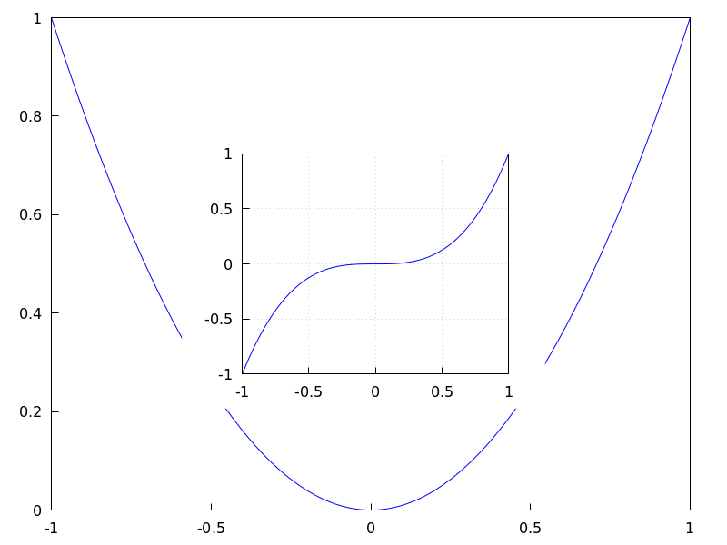
Multiplot with selected dimensions.
(%i1) draw(
terminal = wxt,
gr2d(
grid=[5,5],
allocation = [[0, 0],[1, 1/4]],
explicit(x^2,x,-1,1)),
gr3d(
allocation = [[0, 1/4],[1, 3/4]],
explicit(x^2+y^2,x,-1,1,y,-1,1) ))$
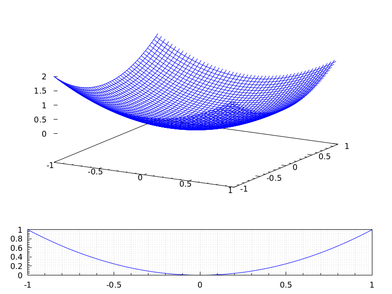
See also option columns.
See also: columns.
axis_3d — Variable
Default value: true
If axis_3d is true, the x, y and z axis are shown in 3d scenes.
Since this is a global graphics option, its position in the scene description does not matter.
Example:
(%i1) draw3d(axis_3d = false,
explicit(sin(x^2+y^2),x,-2,2,y,-2,2) )$
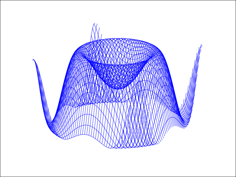
See also axis_bottom, axis_left, axis_top, and axis_right for axis in 2d.
See also: axis_bottom, axis_left, axis_top, axis_right.
axis_bottom — Variable
Default value: true
If axis_bottom is true, the bottom axis is shown in 2d scenes.
Since this is a global graphics option, its position in the scene description does not matter.
Example:
(%i1) draw2d(axis_bottom = false,
explicit(x^3,x,-1,1))$
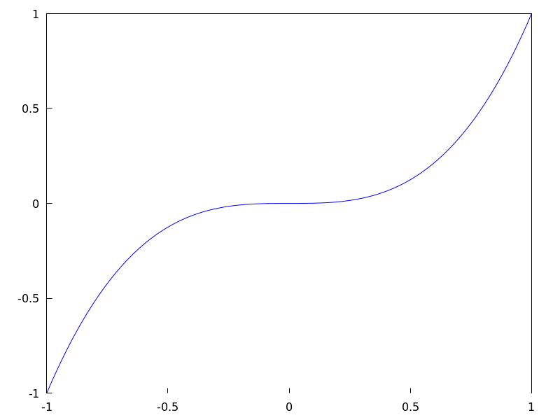
See also axis_left, axis_top, axis_right and axis_005f3d.
See also: axis_left, axis_top, axis_right, axis_3d.
axis_left — Variable
Default value: true
If axis_left is true, the left axis is shown in 2d scenes.
Since this is a global graphics option, its position in the scene description does not matter.
Example:
(%i1) draw2d(axis_left = false,
explicit(x^3,x,-1,1))$
See also axis_bottom, axis_top, axis_right and axis_005f3d.
See also: axis_bottom, axis_top, axis_right, axis_3d.
axis_right — Variable
Default value: true
If axis_right is true, the right axis is shown in 2d scenes.
Since this is a global graphics option, its position in the scene description does not matter.
Example:
(%i1) draw2d(axis_right = false,
explicit(x^3,x,-1,1))$
See also axis_bottom, axis_left, axis_top and axis_005f3d.
See also: axis_bottom, axis_left, axis_top, axis_3d.
axis_top — Variable
Default value: true
If axis_top is true, the top axis is shown in 2d scenes.
Since this is a global graphics option, its position in the scene description does not matter.
Example:
(%i1) draw2d(axis_top = false,
explicit(x^3,x,-1,1))$
See also axis_bottom, axis_left, axis_right, and axis_005f3d.
See also: axis_bottom, axis_left, axis_right, axis_3d.
background_color — Variable
Default value: white
Sets the background color for terminals. Default background color is white.
Since this is a global graphics option, its position in the scene description does not matter.
This option does not work with terminals epslatex and epslatex_standalone.
See also color
bars ([x1, h1, w1], [x2, h2, w2, …]) — Function
Draws vertical bars in 2D.
2D
bars ([x1,h1,w1], [x2,h2,w2, ...])
draws bars centered at values x1, x2, … with heights h1, h2, …
and widths w1, w2, …
This object is affected by the following graphic options: key,
fill_color, fill_density and line_005fwidth.
Example:
(%i1) draw2d(
key = "Group A",
fill_color = blue,
fill_density = 0.2,
bars([0.8,5,0.4],[1.8,7,0.4],[2.8,-4,0.4]),
key = "Group B",
fill_color = red,
fill_density = 0.6,
line_width = 4,
bars([1.2,4,0.4],[2.2,-2,0.4],[3.2,5,0.4]),
xaxis = true);
See also: key, fill_color, fill_density, line_width.
border — Variable
Default value: true
If border is true, borders of polygons are painted
according to line_type and line_width.
This option affects the following graphic objects:
gr2d: polygon, rectangle and ellipse.
Example:
(%i1) draw2d(color = brown,
line_width = 8,
polygon([[3,2],[7,2],[5,5]]),
border = false,
fill_color = blue,
polygon([[5,2],[9,2],[7,5]]) )$
See also: polygon, rectangle, ellipse.
boundaries_array — Variable
Default value: false
boundaries_array is where the graphic object geomap looks
for boundaries coordinates.
Each component of boundaries_array is an array of floating
point quantities, the coordinates of a polygonal segment or map boundary.
See also geomap.
See also: geomap.
capping — Variable
Default value: [false, false]
A list with two possible elements, true and false,
indicating whether the extremes of a graphic object tube remain closed
or open. By default, both extremes are left open.
Setting capping = false is equivalent to capping = [false, false],
and capping = true is equivalent to capping = [true, true].
Example:
(%i1) draw3d(
capping = [false, true],
tube(0, 0, a, 1,
a, 0, 8) )$
cbrange — Variable
Default value: auto
If cbrange is auto, the range for the values which are
colored when enhanced3d is not false is computed
automatically. Values outside of the color range use color of the
nearest extreme.
When enhanced3d or colorbox is false, option cbrange has
no effect.
If the user wants a specific interval for the colored values, it must
be given as a Maxima list, as in cbrange=[-2, 3].
Since this is a global graphics option, its position in the scene description does not matter.
Example:
(%i1) draw3d (
enhanced3d = true,
color = green,
cbrange = [-3,10],
explicit(x^2+y^2, x,-2,2,y,-2,2)) $
See also enhanced3d, colorbox and cbtics.
See also: enhanced3d, colorbox, cbtics.
cbtics — Variable
Default value: auto
This graphic option controls the way tic marks are drawn on the colorbox
when option enhanced3d is not false.
When enhanced3d or colorbox is false, option cbtics has
no effect.
See xtics for a complete description.
Example :
(%i1) draw3d (
enhanced3d = true,
color = green,
cbtics = {["High",10],["Medium",05],["Low",0]},
cbrange = [0, 10],
explicit(x^2+y^2, x,-2,2,y,-2,2)) $
See also enhanced3d, colorbox and cbrange.
See also: enhanced3d, colorbox, cbrange.
colorbox — Variable
Default value: true
If colorbox is true, a color scale without label is drawn together with
image 2D objects, or coloured 3d objects. If colorbox is false, no
color scale is shown. If colorbox is a string, a color scale with label is drawn.
Since this is a global graphics option, its position in the scene description does not matter.
Example:
Color scale and images.
(%i1) im: apply('matrix,
makelist(makelist(random(200),i,1,30),i,1,30))$
(%i2) draw(
gr2d(image(im,0,0,30,30)),
gr2d(colorbox = false, image(im,0,0,30,30))
)$
 Color scale and 3D coloured object.
(%i1) draw3d(
colorbox = "Magnitude",
enhanced3d = true,
explicit(x^2+y^2,x,-1,1,y,-1,1))$
See also palette_005fdraw.
See also: palette_draw.
columns — Variable
Default value: 1
columns is the number of columns in multiple plots.
Since this is a global graphics option, its position in the scene description
does not matter. It can be also used as an argument of function draw.
Example:
(%i1) scene1: gr2d(title="Ellipse",
nticks=30,
parametric(2*cos(t),5*sin(t),t,0,2*%pi))$
(%i2) scene2: gr2d(title="Triangle",
polygon([4,5,7],[6,4,2]))$
(%i3) draw(scene1, scene2, columns = 2)$

contour — Variable
Default value: none
Option contour enables the user to select where to plot contour lines.
Possible values are:
none:
no contour lines are plotted.
base:
contour lines are projected on the xy plane.
surface:
contour lines are plotted on the surface.
both:
two contour lines are plotted: on the xy plane and on the surface.
map:
contour lines are projected on the xy plane, and the view point is
set just in the vertical.
Since this is a global graphics option, its position in the scene description does not matter.
Example:
(%i1) draw3d(explicit(20*exp(-x^2-y^2)-10,x,0,2,y,-3,3),
contour_levels = 15,
contour = both,
surface_hide = true) $
(%i1) draw3d(explicit(20*exp(-x^2-y^2)-10,x,0,2,y,-3,3),
contour_levels = 15,
contour = map
) $
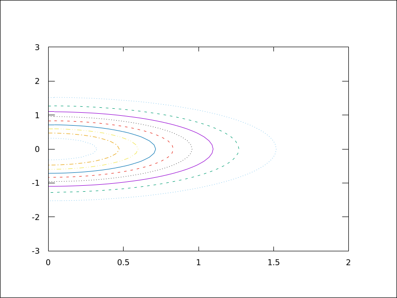
contour_levels — Variable
Default value: 5
This graphic option controls the way contours are drawn.
contour_levels can be set to a positive integer number, a list of three
numbers or an arbitrary set of numbers:
When option contour_levels is bounded to positive integer n,
n contour lines will be drawn at equal intervals. By default, five
equally spaced contours are plotted.
When option contour_levels is bounded to a list of length three of the
form [lowest,s,highest], contour lines are plotted from lowest
to highest in steps of s.
When option contour_levels is bounded to a set of numbers of the
form {n1, n2, ...}, contour lines are plotted at values n1,
n2, …
Since this is a global graphics option, its position in the scene description does not matter.
Examples:
Ten equally spaced contour lines. The actual number of levels can be adjusted to give simple labels.
(%i1) draw3d(color = green,
explicit(20*exp(-x^2-y^2)-10,x,0,2,y,-3,3),
contour_levels = 10,
contour = both,
surface_hide = true) $
From -8 to 8 in steps of 4.
(%i1) draw3d(color = green,
explicit(20*exp(-x^2-y^2)-10,x,0,2,y,-3,3),
contour_levels = [-8,4,8],
contour = both,
surface_hide = true) $
Isolines at levels -7, -6, 0.8 and 5.
(%i1) draw3d(color = green,
explicit(20*exp(-x^2-y^2)-10,x,0,2,y,-3,3),
contour_levels = {-7, -6, 0.8, 5},
contour = both,
surface_hide = true) $
See also contour.
See also: contour.
cylindrical (radius, z, minz, maxz, azi, minazi, maxazi) — Function
Draws 3D functions defined in cylindrical coordinates.
3D
cylindrical(radius, z, minz, maxz, azi, minazi, maxazi) plots the function radius(z, azi) defined in cylindrical coordinates, with variable z taking
values from minz to maxz and azimuth azi taking values
from minazi to maxazi.
This object is affected by the following graphic options: xu_grid,
yv_grid, line_type, key, wired_surface, enhanced3d and color
Example:
(%i1) draw3d(cylindrical(1,z,-2,2,az,0,2*%pi))$
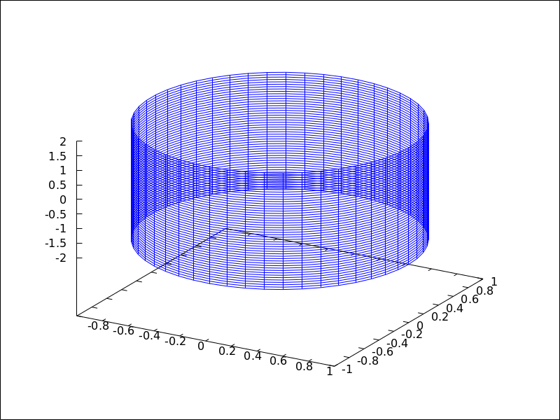
See also: xu_grid, yv_grid, line_type, key, wired_surface.
data_file_name — Variable
Default value: "data.gnuplot"
This is the name of the file with the numeric data needed by Gnuplot to build the requested plot.
Since this is a global graphics option, its position in the scene description
does not matter. It can be also used as an argument of function draw.
See example in gnuplot_file_name.
delay — Variable
Default value: 5
This is the delay in 1/100 seconds of frames in animated gif files.
Since this is a global graphics option, its position in the scene description
does not matter. It can be also used as an argument of function draw.
Example:
(%i1) draw(
delay = 100,
file_name = "zzz",
terminal = 'animated_gif,
gr2d(explicit(x^2,x,-1,1)),
gr2d(explicit(x^3,x,-1,1)),
gr2d(explicit(x^4,x,-1,1)));
End of animation sequence
(%o2) [gr2d(explicit), gr2d(explicit), gr2d(explicit)]
Option delay is only active in animated gif’s; it is ignored in
any other case.
See also terminal, and dimensions.
See also: terminal.
dimensions — Variable
Default value: [600,500]
Dimensions of the output terminal. Its value is a list formed by the width and the height. The meaning of the two numbers depends on the terminal you are working with.
With terminals gif, animated_gif, png, jpg,
svg, screen, wxt, qt, x11,
windows and aquaterm, the integers represent the number of
points in each direction. If they are not integers, they are rounded.
With terminals eps, epslatex, epslatex_standalone,
eps_color, multipage_eps, multipage_eps_color,
cairolatex_pdf, cairolatex_pdf_standalone,
pdf, multipage_pdf, pdfcairo,
multipage_pdfcairo, tikz, and tikz_standalone, both
numbers represent hundredths of cm, which means that, by default,
pictures in these formats are 6 cm in width and 5 cm in height.
Since this is a global graphics option, its position in the scene description
does not matter. It can be also used as an argument of function draw.
Examples:
Option dimensions applied to file output
and to wxt canvas.
(%i1) draw2d(
dimensions = [300,300],
terminal = 'png,
explicit(x^4,x,-1,1)) $
(%i2) draw2d(
dimensions = [300,300],
terminal = 'wxt,
explicit(x^4,x,-1,1)) $
Option dimensions applied to eps output.
We want an eps file with A4 portrait dimensions.
(%i1) A4portrait: 100*[21, 29.7]$
(%i2) draw3d(
dimensions = A4portrait,
terminal = 'eps,
explicit(x^2-y^2,x,-2,2,y,-2,2)) $
draw (<arg_1>, …) — Function
Plots a series of scenes; its arguments are gr2d and/or gr3d
objects, together with some options, or lists of scenes and options.
By default, the scenes are put together
in one column.
Besides scenes the function draw accepts the following global options:
terminal, columns, dimensions, file_name
and delay.
Functions draw2d and draw3d short cuts that can be used
when only one scene is required, in two or three dimensions, respectively.
See also gr2d and gr3d.
Examples:
(%i1) scene1: gr2d(title="Ellipse",
nticks=300,
parametric(2*cos(t),5*sin(t),t,0,2*%pi))$
(%i2) scene2: gr2d(title="Triangle",
polygon([4,5,7],[6,4,2]))$
(%i3) draw(scene1, scene2, columns = 2)$
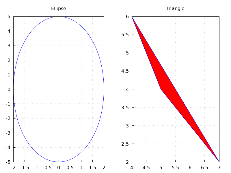
(%i1) scene1: gr2d(title="A sinus",
grid=true,
explicit(sin(t),t,0,2*%pi))$
(%i2) scene2: gr2d(title="A cosinus",
grid=true,
explicit(cos(t),t,0,2*%pi))$
(%i3) draw(scene1, scene2)$
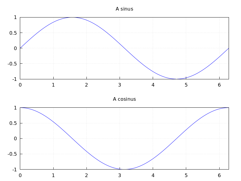
The following two draw sentences are equivalent:
(%i1) draw(gr3d(explicit(x^2+y^2,x,-1,1,y,-1,1)));
(%o1) [gr3d(explicit)]
(%i2) draw3d(explicit(x^2+y^2,x,-1,1,y,-1,1));
(%o2) [gr3d(explicit)]
Creating an animated gif file:
(%i1) draw(
delay = 100,
file_name = "zzz",
terminal = 'animated_gif,
gr2d(explicit(x^2,x,-1,1)),
gr2d(explicit(x^3,x,-1,1)),
gr2d(explicit(x^4,x,-1,1)));
End of animation sequence
(%o1) [gr2d(explicit), gr2d(explicit), gr2d(explicit)]
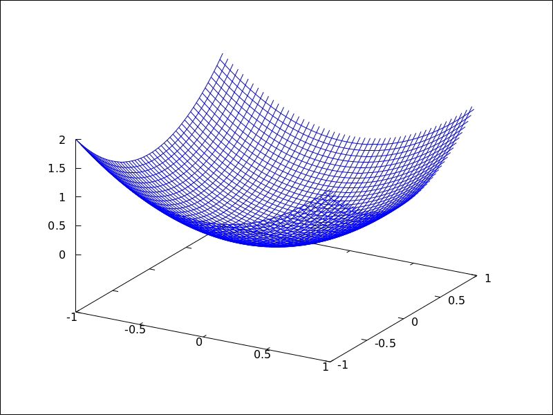 See also
 gr2d, gr3d, draw2d and draw3d.
See also: terminal, columns, dimensions, file_name, delay, draw2d, draw3d, gr2d, gr3d.
draw2d (argument_1, …) — Function
This function is a shortcut for
draw(gr2d(options, ..., graphic_object, ...)).
It can be used to plot a unique scene in 2d, as can be seen in most examples below.
See also draw and gr2d.
See also: draw, gr2d.
draw3d (argument_1, …) — Function
This function is a shortcut for
draw(gr3d(options, ..., graphic_object, ...)).
It can be used to plot a unique scene in 3d, as can be seen in many examples below.
See also draw and gr3d.
See also: draw, gr3d.
draw_file (graphic option, …, graphic object, …) — Function
Saves the current plot into a file. Accepted graphics options are:
terminal, dimensions and file_name.
Example:
(%i1) /* screen plot */
draw(gr3d(explicit(x^2+y^2,x,-1,1,y,-1,1)))$
(%i2) /* same plot in eps format */
draw_file(terminal = eps,
dimensions = [5,5]) $
draw_realpart — Variable
Default value: true
When true, functions to be drawn are considered as complex functions whose
real part value should be plotted; when false, nothing will be plotted when
the function does not give a real value.
This option affects objects explicit and parametric in 2D and 3D, and
parametric_005fsurface.
Example:
(%i1) draw2d(
draw_realpart = false,
explicit(sqrt(x^2 - 4*x) - x, x, -1, 5),
color = red,
draw_realpart = true,
parametric(x,sqrt(x^2 - 4*x) - x + 1, x, -1, 5) );
See also: explicit, parametric, parametric_surface.
draw_renderer — Variable
Default value: gnuplot_pipes
The only permitted values are gnuplot_pipes, gnuplot,
vtk, vtk6 or vtk7. When draw_renderer is set
to vtk, the VTK interface is used for draw.
elevation_grid (mat, x0, y0, width, height) — Function
Draws matrix mat in 3D space. z values are taken from mat, the abscissas range from x0 to $x0 + width$ and ordinates from y0 to $y0 + height$. Element $a(1,1)$ is projected on point $(x0,y0+height)$, $a(1,n)$ on $(x0+width,y0+height)$, $a(m,1)$ on $(x0,y0)$, and $a(m,n)$ on $(x0+width,y0)$.
This object is affected by the following graphic options: line_type,,
line_width key, wired_surface, enhanced3d and color
In older versions of Maxima, elevation_grid was called mesh.
See also mesh.
Example:
(%i1) m: apply(
matrix,
makelist(makelist(random(10.0),k,1,30),i,1,20)) $
(%i2) draw3d(
color = blue,
elevation_grid(m,0,0,3,2),
xlabel = "x",
ylabel = "y",
surface_hide = true);
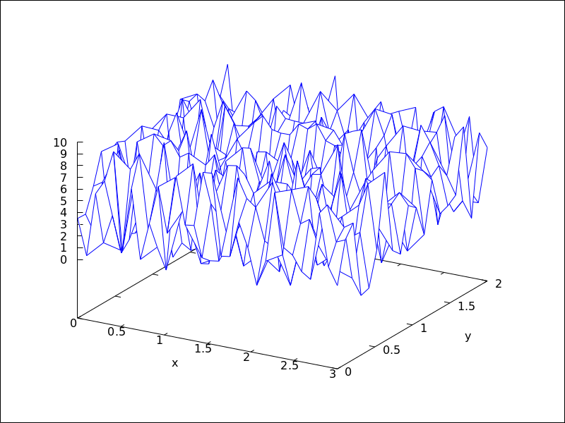
See also: line_type, line_width, key, wired_surface, enhanced3d, elevation_grid, mesh.
ellipse (xc, yc, a, b, ang1, ang2) — Function
Draws ellipses and circles in 2D.
2D
ellipse (xc, yc, a, b, ang1, ang2)
plots an ellipse centered at [xc, yc] with horizontal and vertical
semi axis a and b, respectively, starting at angle ang1 with an amplitude
equal to angle ang2.
This object is affected by the following graphic options: nticks,
transparent, fill_color, fill_density, border, line_width,
line_type, key and color
Example:
(%i1) draw2d(transparent = false,
fill_color = red,
color = gray30,
transparent = false,
line_width = 5,
ellipse(0,6,3,2,270,-270),
/* center (x,y), a, b, start & end in degrees */
transparent = true,
color = blue,
line_width = 3,
ellipse(2.5,6,2,3,30,-90),
xrange = [-3,6],
yrange = [2,9] )$
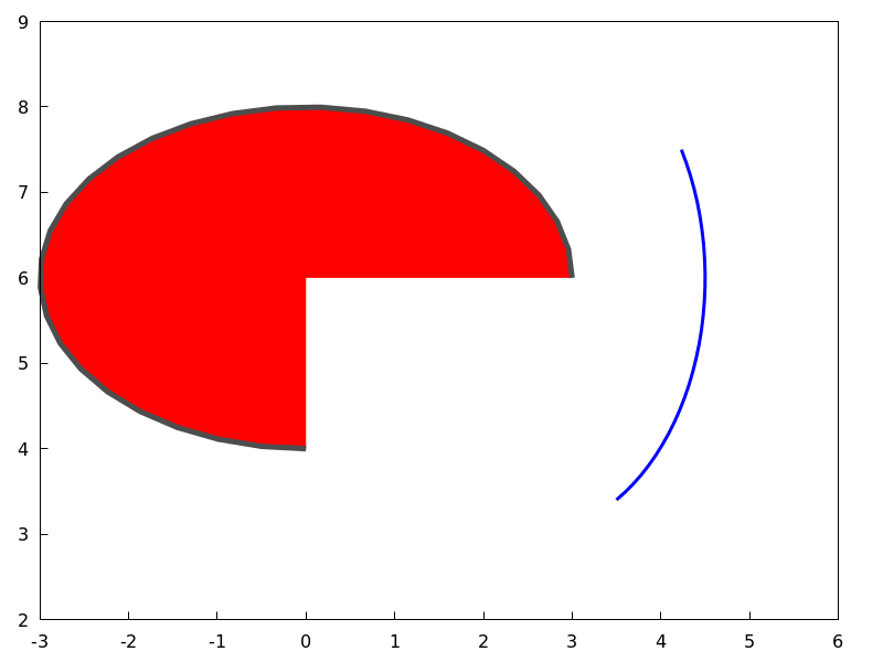
See also: nticks, transparent, fill_color, fill_density, border, line_type, key.
enhanced3d — Variable
Default value: none
If enhanced3d is none, surfaces are not colored in 3D plots.
In order to get a colored surface, a list must be assigned to option
enhanced3d, where the first element is an expression and the rest
are the names of the variables or parameters used in that expression. A list such
[f(x,y,z), x, y, z] means that point [x,y,z] of the surface
is assigned number f(x,y,z), which will be colored according to
the actual palette. For those 3D graphic objects defined in terms of
parameters, it is possible to define the color number in terms of
the parameters, as in [f(u), u], as in objects parametric and
tube, or [f(u,v), u, v], as in object parametric_surface.
While all 3D objects admit the model based on absolute coordinates,
[f(x,y,z), x, y, z], only two of them, namely explicit
and elevation_grid, accept also models defined on the [x,y] coordinates,
[f(x,y), x, y]. 3D graphic object implicit accepts only the
[f(x,y,z), x, y, z] model. Object points accepts also the
[f(x,y,z), x, y, z] model, but when points have a chronological nature,
model [f(k), k] is also valid, being k an ordering parameter.
When enhanced3d is assigned something different to none, options
color and surface_hide are ignored.
The names of the variables defined in the lists may be different to those used in the definitions of the graphic objects.
In order to maintain back compatibility, enhanced3d = false is equivalent
to enhanced3d = none, and enhanced3d = true is equivalent to
enhanced3d = [z, x, y, z]. If an expression is given to enhanced3d,
its variables must be the same used in the surface definition. This is not
necessary when using lists.
See option palette to learn how palettes are specified.
Examples:
explicit object with coloring defined by the [f(x,y,z), x, y, z] model.
(%i1) draw3d(
enhanced3d = [x-z/10,x,y,z],
palette = gray,
explicit(20*exp(-x^2-y^2)-10,x,-3,3,y,-3,3))$
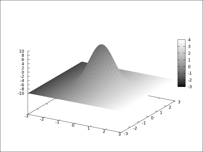
explicit object with coloring defined by the [f(x,y), x, y] model.
The names of the variables defined in the lists may be different to those
used in the definitions of the graphic objects; in this case, r corresponds
to x, and s to y.
(%i1) draw3d(
enhanced3d = [sin(r*s),r,s],
explicit(20*exp(-x^2-y^2)-10,x,-3,3,y,-3,3))$

parametric object with coloring defined by the [f(x,y,z), x, y, z] model.
(%i1) draw3d(
nticks = 100,
line_width = 2,
enhanced3d = [if y>= 0 then 1 else 0, x, y, z],
parametric(sin(u)^2,cos(u),u,u,0,4*%pi)) $
parametric object with coloring defined by the [f(u), u] model.
In this case, (u-1)^2 is a shortcut for [(u-1)^2,u].
(%i1) draw3d(
nticks = 60,
line_width = 3,
enhanced3d = (u-1)^2,
parametric(cos(5*u)^2,sin(7*u),u-2,u,0,2))$
elevation_grid object with coloring defined by the [f(x,y), x, y] model.
(%i1) m: apply(
matrix,
makelist(makelist(cos(i^2/80-k/30),k,1,30),i,1,20)) $
(%i2) draw3d(
enhanced3d = [cos(x*y*10),x,y],
elevation_grid(m,-1,-1,2,2),
xlabel = "x",
ylabel = "y");
tube object with coloring defined by the [f(x,y,z), x, y, z] model.
(%i1) draw3d(
enhanced3d = [cos(x-y),x,y,z],
palette = gray,
xu_grid = 50,
tube(cos(a), a, 0, 1, a, 0, 4*%pi) )$
tube object with coloring defined by the [f(u), u] model.
Here, enhanced3d = -a would be the shortcut for enhanced3d = [-foo,foo].
(%i1) draw3d(
capping = [true, false],
palette = [26,15,-2],
enhanced3d = [-foo, foo],
tube(a, a, a^2, 1, a, -2, 2) )$
implicit and points objects with coloring defined by the [f(x,y,z), x, y, z] model.
(%i1) draw3d(
enhanced3d = [x-y,x,y,z],
implicit((x^2+y^2+z^2-1)*(x^2+(y-1.5)^2+z^2-0.5)=0.015,
x,-1,1,y,-1.2,2.3,z,-1,1)) $
(%i2) m: makelist([random(1.0),random(1.0),random(1.0)],k,1,2000)$
(%i3) draw3d(
point_type = filled_circle,
point_size = 2,
enhanced3d = [u+v-w,u,v,w],
points(m) ) $
When points have a chronological nature, model [f(k), k] is also valid,
being k an ordering parameter.
(%i1) m:makelist([random(1.0), random(1.0), random(1.0)],k,1,5)$
(%i2) draw3d(
enhanced3d = [sin(j), j],
point_size = 3,
point_type = filled_circle,
points_joined = true,
points(m)) $
See also: enhanced3d, parametric, tube, elevation_grid.
error_type — Variable
Default value: y
Depending on its value, which can be x, y, or xy,
graphic object errors will draw points with horizontal, vertical,
or both, error bars. When error_type=boxes, boxes will be drawn
instead of crosses.
See also errors.
See also: errors.
errors ([x1, x2, …], [y1, y2, …]) — Function
Draws points with error bars, horizontally, vertically or both, depending on the
value of option error_type.
2D
If error_type = x, arguments to errors must be of the form
[x, y, xdelta] or [x, y, xlow, xhigh]. If error_type = y,
arguments must be of the form [x, y, ydelta] or
[x, y, ylow, yhigh]. If error_type = xy or
error_type = boxes, arguments to errors must be of the form
[x, y, xdelta, ydelta] or [x, y, xlow, xhigh, ylow, yhigh].
See also error_005ftype.
This object is affected by the following graphic options: error_type,points_joined, line_width, key, line_type,color fill_density, xaxis_secondary and yaxis_005fsecondary.
Option fill_density is only relevant when error_type=boxes.
Examples:
Horizontal error bars.
(%i1) draw2d(
error_type = 'y,
errors([[1,2,1], [3,5,3], [10,3,1], [17,6,2]]))$
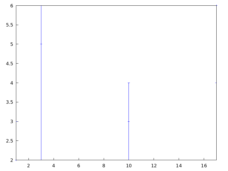
Vertical and horizontal error bars.
(%i1) draw2d(
error_type = 'xy,
points_joined = true,
color = blue,
errors([[1,2,1,2], [3,5,2,1], [10,3,1,1], [17,6,1/2,2]]));
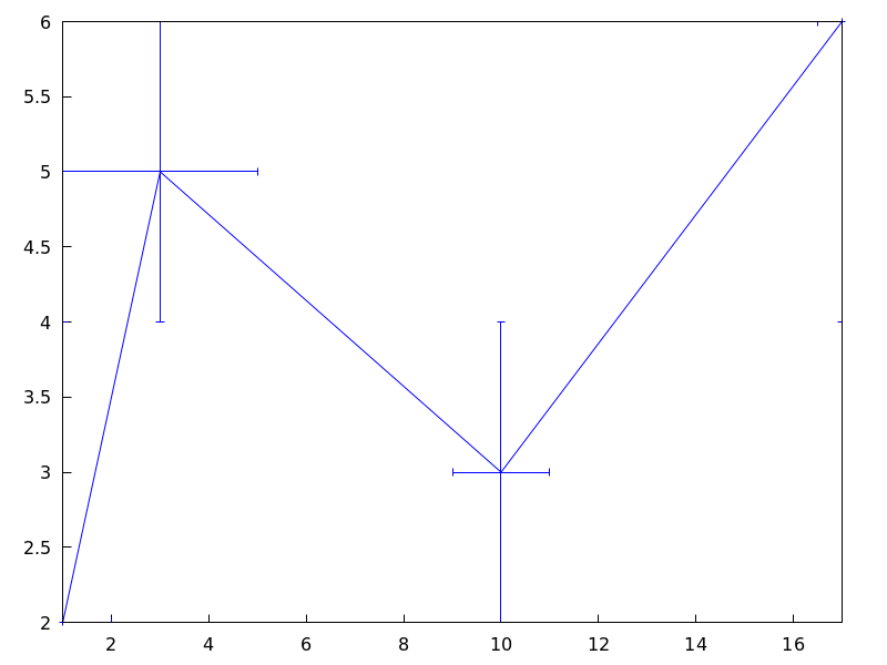
See also: error_type, points_joined, line_width, key, line_type, fill_density, xaxis_secondary, yaxis_secondary.
explicit (expr, var, minval, maxval) — Function
Draws explicit functions in 2D and 3D.
2D
explicit(fcn,var,minval,maxval) plots explicit function fcn,
with variable var taking values from minval to maxval.
This object is affected by the following graphic options: nticks,
adapt_depth, draw_realpart, line_width, line_type, key,
filled_func, fill_color, fill_density, and color
Example:
(%i1) draw2d(line_width = 3,
color = blue,
explicit(x^2,x,-3,3) )$
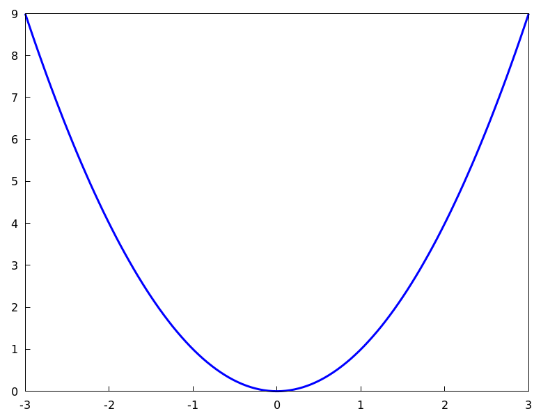
(%i2) draw2d(fill_color = brown,
filled_func = true,
explicit(x^2,x,-3,3) )$
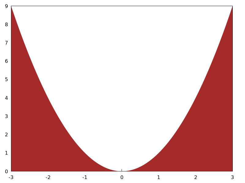
3D
explicit(fcn, var1, minval1, maxval1, var2, minval2, maxval2) plots the explicit function fcn, with
variable var1 taking values from minval1 to maxval1 and
variable var2 taking values from minval2 to maxval2.
This object is affected by the following graphic options: draw_realpart, xu_grid,
yv_grid, line_type, line_width, key, wired_surface,
enhanced3d and color.
Example:
(%i1) draw3d(key = "Gauss",
color = "#a02c00",
explicit(20*exp(-x^2-y^2)-10,x,-3,3,y,-3,3),
yv_grid = 10,
color = blue,
key = "Plane",
explicit(x+y,x,-5,5,y,-5,5),
surface_hide = true)$
See also filled_func for filled functions.
See also: nticks, draw_realpart, line_width, line_type, key, filled_func, fill_color, fill_density, xu_grid, yv_grid, wired_surface, enhanced3d.
file_name — Variable
Default value: "maxima_out"
This is the name of the file where terminals png, jpg, gif,
eps, eps_color, pdf, pdfcairo and svg
will save the graphic.
Since this is a global graphics option, its position in the scene description
does not matter. It can be also used as an argument of function draw.
Example:
(%i1) draw2d(file_name = "myfile",
explicit(x^2,x,-1,1),
terminal = 'png)$
See also terminal, dimensions_005fdraw.
See also: terminal, dimensions_draw.
fill_color — Variable
Default value: "red"
fill_color specifies the color for filling polygons and
2d explicit functions.
See color to learn how colors are specified.
fill_density — Variable
Default value: 0
fill_density is a number between 0 and 1 that specifies
the intensity of the fill_color in bars objects.
See bars for examples.
filled_func — Variable
Default value: false
Option filled_func controls how regions limited by functions
should be filled. When filled_func is true, the region
bounded by the function defined with object explicit and the
bottom of the graphic window is filled with fill_color. When
filled_func contains a function expression, then the region bounded
by this function and the function defined with object explicit
will be filled. By default, explicit functions are not filled.
A useful special case is filled_func=0, which generates the region
bond by the horizontal axis and the explicit function.
This option affects only the 2d graphic object explicit.
Example:
Region bounded by an explicit object and the bottom of the
graphic window.
(%i1) draw2d(fill_color = red,
filled_func = true,
explicit(sin(x),x,0,10) )$
Region bounded by an explicit object and the function
defined by option filled_func. Note that the variable in
filled_func must be the same as that used in explicit.
(%i1) draw2d(fill_color = grey,
filled_func = sin(x),
explicit(-sin(x),x,0,%pi));
 See also
 fill_color and explicit.
See also: explicit, fill_color.
font — Variable
Default value: "" (empty string)
This option can be used to set the font face to be used by the terminal. Only one font face and size can be used throughout the plot.
Since this is a global graphics option, its position in the scene description does not matter.
See also font_005fsize.
Gnuplot doesn’t handle fonts by itself, it leaves this task to the support libraries of the different terminals, each one with its own philosophy about it. A brief summary follows:
x11: Uses the normal x11 font server mechanism.
Example:
(%i1) draw2d(font = "Arial",
font_size = 20,
label(["Arial font, size 20",1,1]))$
windows: The windows terminal doesn’t support changing of fonts from inside the plot. Once the plot has been generated, the font can be changed right-clicking on the menu of the graph window.
png, jpeg, gif:
The libgd library uses the font path stored in the environment
variable GDFONTPATH; in this case, it is only necessary to
set option font to the font’s name. It is also possible to
give the complete path to the font file.
Examples:
Option font can be given the complete path to the font file:
(%i1) path: "/usr/share/fonts/truetype/freefont/" $
(%i2) file: "FreeSerifBoldItalic.ttf" $
(%i3) draw2d(
font = concat(path, file),
font_size = 20,
color = red,
label(["FreeSerifBoldItalic font, size 20",1,1]),
terminal = png)$
If environment variable GDFONTPATH is set to the
path where font files are allocated, it is possible to
set graphic option font to the name of the font.
(%i1) draw2d(
font = "FreeSerifBoldItalic",
font_size = 20,
color = red,
label(["FreeSerifBoldItalic font, size 20",1,1]),
terminal = png)$
Postscript:
Standard Postscript fonts are:
"Times-Roman", "Times-Italic", "Times-Bold",
"Times-BoldItalic",
"Helvetica", "Helvetica-Oblique", "Helvetica-Bold",
"Helvetic-BoldOblique", "Courier",
"Courier-Oblique", "Courier-Bold",
and "Courier-BoldOblique".
Example:
(%i1) draw2d(
font = "Courier-Oblique",
font_size = 15,
label(["Courier-Oblique font, size 15",1,1]),
terminal = eps)$
pdf: Uses same fonts as Postscript.
pdfcairo: Uses same fonts as wxt.
wxt:
The pango library finds fonts via the fontconfig utility.
aqua:
Default is "Times-Roman".
The gnuplot documentation is an important source of information about terminals and fonts.
See also: font_size.
font_size — Variable
Default value: 10
This option can be used to set the font size to be used by the terminal.
Only one font face and size can be used throughout the plot. font_size is
active only when option font is not equal to the empty string.
Since this is a global graphics option, its position in the scene description does not matter.
See also font.
See also: font.
geomap (numlist) — Function
Draws cartographic maps in 2D and 3D.
2D
This function works together with global variable boundaries_array.
Argument numlist is a list containing numbers or lists of numbers.
All these numbers must be integers greater or equal than zero,
representing the components of global array boundaries_array.
Each component of boundaries_array is an array of floating
point quantities, the coordinates of a polygonal segment or map boundary.
geomap (numlist) flattens its arguments and draws the
associated boundaries in boundaries_array.
This object is affected by the following graphic options: line_width,
line_type and color.
Examples:
A simple map defined by hand:
(%i1) load("worldmap")$
(%i2) /* Vertices of boundary #0: {(1,1),(2,5),(4,3)} */
( bnd0: make_array(flonum,6),
bnd0[0]:1.0, bnd0[1]:1.0, bnd0[2]:2.0,
bnd0[3]:5.0, bnd0[4]:4.0, bnd0[5]:3.0 )$
(%i3) /* Vertices of boundary #1: {(4,3),(5,4),(6,4),(5,1)} */
( bnd1: make_array(flonum,8),
bnd1[0]:4.0, bnd1[1]:3.0, bnd1[2]:5.0, bnd1[3]:4.0,
bnd1[4]:6.0, bnd1[5]:4.0, bnd1[6]:5.0, bnd1[7]:1.0)$
(%i4) /* Vertices of boundary #2: {(5,1), (3,0), (1,1)} */
( bnd2: make_array(flonum,6),
bnd2[0]:5.0, bnd2[1]:1.0, bnd2[2]:3.0,
bnd2[3]:0.0, bnd2[4]:1.0, bnd2[5]:1.0 )$
(%i5) /* Vertices of boundary #3: {(1,1), (4,3)} */
( bnd3: make_array(flonum,4),
bnd3[0]:1.0, bnd3[1]:1.0, bnd3[2]:4.0, bnd3[3]:3.0)$
(%i6) /* Vertices of boundary #4: {(4,3), (5,1)} */
( bnd4: make_array(flonum,4),
bnd4[0]:4.0, bnd4[1]:3.0, bnd4[2]:5.0, bnd4[3]:1.0)$
(%i7) /* Pack all together in boundaries_array */
( boundaries_array: make_array(any,5),
boundaries_array[0]: bnd0, boundaries_array[1]: bnd1,
boundaries_array[2]: bnd2, boundaries_array[3]: bnd3,
boundaries_array[4]: bnd4 )$
(%i8) draw2d(geomap([0,1,2,3,4]))$
The auxiliary package worldmap sets the global variable
boundaries_array to real world boundaries in
(longitude, latitude) coordinates. These data are in the
public domain and come from
https://web.archive.org/web/20100310124019/http://www-cger.nies.go.jp/grid-e/gridtxt/grid19.html.
Package worldmap defines also boundaries for countries,
continents and coastlines as lists with the necessary components of
boundaries_array (see file share/draw/worldmap.mac
for more information). Package worldmap automatically loads
package worldmap.
(%i1) load("worldmap")$
(%i2) c1: gr2d(geomap([Canada,United_States,
Mexico,Cuba]))$
(%i3) c2: gr2d(geomap(Africa))$
(%i4) c3: gr2d(geomap([Oceania,China,Japan]))$
(%i5) c4: gr2d(geomap([France,Portugal,Spain,
Morocco,Western_Sahara]))$
(%i6) draw(columns = 2,
c1,c2,c3,c4)$
Package worldmap is also useful for plotting
countries as polygons. In this case, graphic object
geomap is no longer necessary and the polygon
object is used instead. Since lists are now used and not
arrays, maps rendering will be slower. See also make_poly_country
and make_poly_continent to understand the following code.
(%i1) load("worldmap")$
(%i2) mymap: append(
[color = white], /* borders are white */
[fill_color = red], make_poly_country(Bolivia),
[fill_color = cyan], make_poly_country(Paraguay),
[fill_color = green], make_poly_country(Colombia),
[fill_color = blue], make_poly_country(Chile),
[fill_color = "#23ab0f"], make_poly_country(Brazil),
[fill_color = goldenrod], make_poly_country(Argentina),
[fill_color = "midnight-blue"], make_poly_country(Uruguay))$
(%i3) apply(draw2d, mymap)$
3D
geomap (numlist) projects map boundaries on the sphere of radius 1
centered at (0,0,0). It is possible to change the sphere or the projection type
by using geomap (numlist,3Dprojection).
Available 3D projections:
[spherical_projection,x,y,z,r]: projects map boundaries on the sphere of
radius r centered at (x,y,z).
(%i1) load("worldmap")$
(%i2) draw3d(geomap(Australia), /* default projection */
geomap(Australia,
[spherical_projection,2,2,2,3]))$
[cylindrical_projection,x,y,z,r,rc]: re-projects spherical map boundaries on the cylinder of radius
rc and axis passing through the poles of the globe of radius r centered at (x,y,z).
(%i1) load("worldmap")$
(%i2) draw3d(geomap([America_coastlines,Eurasia_coastlines],
[cylindrical_projection,2,2,2,3,4]))$
[conic_projection,x,y,z,r,alpha]: re-projects spherical map boundaries on the cones of angle alpha,
with axis passing through the poles of the globe of radius r centered at (x,y,z). Both
the northern and southern cones are tangent to sphere.
(%i1) load("worldmap")$
(%i2) draw3d(geomap(World_coastlines,
[conic_projection,0,0,0,1,90]))$
See also https://riotorto.users.sourceforge.net/Maxima/gnuplot/geomap/ for more elaborated examples.
See also: line_width, line_type, make_poly_country, make_poly_continent.
get_pixel (pic, x, y) — Function
Returns pixel from picture. Coordinates x and y range from 0 to
width-1 and height-1, respectively.
gnuplot_file_name — Variable
Default value: "maxout_xxx.gnuplot" with "xxx"
being a number that is unique to each concurrently-running
maxima process.
This is the name of the file with the necessary commands to be processed by Gnuplot.
Since this is a global graphics option, its position in the scene description
does not matter. It can be also used as an argument of function draw.
Example:
(%i1) draw2d(
file_name = "my_file",
gnuplot_file_name = "my_commands_for_gnuplot",
data_file_name = "my_data_for_gnuplot",
terminal = png,
explicit(x^2,x,-1,1)) $
See also data_005ffile_005fname.
See also: data_file_name.
gr2d (argument_1, …) — Function
Function gr2d builds an object describing a 2D scene. Arguments are
graphic options, graphic objects, or lists containing both graphic options and objects.
This scene is interpreted sequentially: graphic options affect those graphic objects
placed on its right. Some graphic options affect the global appearance of the scene.
This is the list of graphic objects available for scenes in two dimensions:
bars, ellipse, explicit, image, implicit, label,
parametric, points, polar, polygon, quadrilateral,
rectangle, triangle, vector and geomap
(this one defined in package worldmap).
See also draw
and draw2d.
(%i1) draw(
gr2d(
key="sin (x)",grid=[2,2],
explicit(
sin(x),
x,0,2*%pi
)
),
gr2d(
key="cos (x)",grid=[2,2],
explicit(
cos(x),
x,0,2*%pi
)
)
);
(%o1) [gr2d(explicit), gr2d(explicit)]
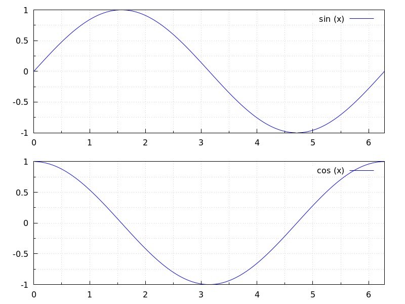
See also: bars, ellipse, explicit, image, implicit, label, parametric, points, polar, polygon, quadrilateral, rectangle, triangle, vector, draw, draw2d.
gr3d (argument_1, …) — Function
Function gr3d builds an object describing a 3d scene. Arguments are
graphic options, graphic objects, or lists containing both graphic options
and objects. This scene is interpreted sequentially: graphic options affect those
graphic objects placed on its right. Some graphic options affect the global
appearance of the scene.
This is the list of graphic objects available for scenes in three dimensions:
cylindrical, elevation_grid, explicit, implicit,
label, mesh, parametric,
parametric_surface, points, quadrilateral,
spherical, triangle, tube,
vector, and geomap (this one defined in package worldmap).
See also draw and draw3d.
See also: cylindrical, elevation_grid, explicit, implicit, label, mesh, parametric, parametric_surface, points, quadrilateral, spherical, triangle, tube, vector, geomap, draw, draw3d.
head_angle — Variable
Default value: 45
head_angle indicates the angle, in degrees, between the arrow heads and
the segment.
This option is relevant only for vector objects.
Example:
(%i1) draw2d(xrange = [0,10],
yrange = [0,9],
head_length = 0.7,
head_angle = 10,
vector([1,1],[0,6]),
head_angle = 20,
vector([2,1],[0,6]),
head_angle = 30,
vector([3,1],[0,6]),
head_angle = 40,
vector([4,1],[0,6]),
head_angle = 60,
vector([5,1],[0,6]),
head_angle = 90,
vector([6,1],[0,6]),
head_angle = 120,
vector([7,1],[0,6]),
head_angle = 160,
vector([8,1],[0,6]),
head_angle = 180,
vector([9,1],[0,6]) )$
See also head_both, head_length, and head_005ftype.
See also: head_both, head_length, head_type.
head_both — Variable
Default value: false
If head_both is true, vectors are plotted with two arrow heads.
If false, only one arrow is plotted.
This option is relevant only for vector objects.
Example:
(%i1) draw2d(xrange = [0,8],
yrange = [0,8],
head_length = 0.7,
vector([1,1],[6,0]),
head_both = true,
vector([1,7],[6,0]) )$
See also head_length, head_angle, and head_005ftype.
See also: head_length, head_angle, head_type.
head_length — Variable
Default value: 2
head_length indicates, in x-axis units, the length of arrow heads.
This option is relevant only for vector objects.
Example:
(%i1) draw2d(xrange = [0,12],
yrange = [0,8],
vector([0,1],[5,5]),
head_length = 1,
vector([2,1],[5,5]),
head_length = 0.5,
vector([4,1],[5,5]),
head_length = 0.25,
vector([6,1],[5,5]))$
See also head_both, head_angle, and head_005ftype.
See also: head_both, head_angle, head_type.
head_type — Variable
Default value: filled
head_type is used to specify how arrow heads are plotted. Possible
values are: filled (closed and filled arrow heads), empty
(closed but not filled arrow heads), and nofilled (open arrow heads).
This option is relevant only for vector objects.
Example:
(%i1) draw2d(xrange = [0,12],
yrange = [0,10],
head_length = 1,
vector([0,1],[5,5]), /* default type */
head_type = 'empty,
vector([3,1],[5,5]),
head_type = 'nofilled,
vector([6,1],[5,5]))$
See also head_both, head_angle, and head_005flength.
See also: head_both, head_angle, head_length.
image (im, x0, y0, width, height) — Function
Renders images in 2D.
2D
image (im,x0,y0,width,height) plots image im in the rectangular
region from vertex (x0,y0) to (x0+width,y0+height) on the real
plane. Argument im must be a matrix of real numbers, a matrix of
vectors of length three or a picture object.
If im is a matrix of real numbers or a levels picture object,
pixel values are interpreted according to graphic option palette,
which is a vector of length three with components
ranging from -36 to +36; each value is an index for a formula mapping the levels
onto red, green and blue colors, respectively:
0: 0 1: 0.5 2: 1
3: x 4: x^2 5: x^3
6: x^4 7: sqrt(x) 8: sqrt(sqrt(x))
9: sin(90x) 10: cos(90x) 11: |x-0.5|
12: (2x-1)^2 13: sin(180x) 14: |cos(180x)|
15: sin(360x) 16: cos(360x) 17: |sin(360x)|
18: |cos(360x)| 19: |sin(720x)| 20: |cos(720x)|
21: 3x 22: 3x-1 23: 3x-2
24: |3x-1| 25: |3x-2| 26: (3x-1)/2
27: (3x-2)/2 28: |(3x-1)/2| 29: |(3x-2)/2|
30: x/0.32-0.78125 31: 2*x-0.84
32: 4x;1;-2x+1.84;x/0.08-11.5
33: |2*x - 0.5| 34: 2*x 35: 2*x - 0.5
36: 2*x - 1
negative numbers mean negative colour component.
palette = gray and palette = color are short cuts for
palette = [3,3,3] and palette = [7,5,15], respectively.
If im is a matrix of vectors of length three or an rgb picture object, they are interpreted as red, green and blue color components.
Examples:
If im is a matrix of real numbers, pixel values are interpreted according
to graphic option palette.
(%i1) im: apply(
'matrix,
makelist(makelist(random(200),i,1,30),i,1,30))$
(%i2) /* palette = color, default */
draw2d(image(im,0,0,30,30))$
(%i3) draw2d(palette = gray, image(im,0,0,30,30))$
(%i4) draw2d(palette = [15,20,-4],
colorbox=false,
image(im,0,0,30,30))$

See also colorbox.
If im is a matrix of vectors of length three, they are interpreted as red, green and blue color components.
(%i1) im: apply(
'matrix,
makelist(
makelist([random(300),
random(300),
random(300)],i,1,30),i,1,30))$
(%i2) draw2d(image(im,0,0,30,30))$

Package draw automatically loads package picture. In this
example, a level picture object is built by hand and then rendered.
(%i1) im: make_level_picture([45,87,2,134,204,16],3,2);
(%o1) picture(level, 3, 2, {Array: #(45 87 2 134 204 16)})
(%i2) /* default color palette */
draw2d(image(im,0,0,30,30))$
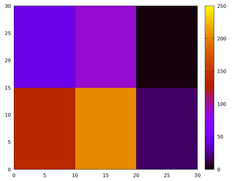
(%i3) /* gray palette */
draw2d(palette = gray,
image(im,0,0,30,30))$
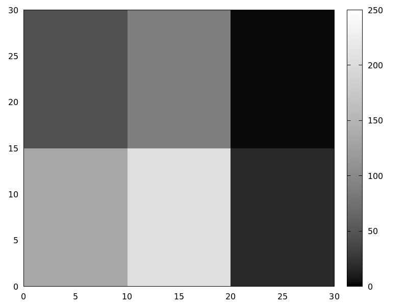
An xpm file is read and then rendered.
(%i1) im: read_xpm("myfile.xpm")$
(%i2) draw2d(image(im,0,0,10,7))$
See also make_level_picture, make_rgb_picture and read_005fxpm.
http://www.telefonica.net/web2/biomates/maxima/gpdraw/image
contains more elaborated examples.
See also: colorbox, make_level_picture, make_rgb_picture, read_xpm.
implicit (fcn, x, xmin, xmax, y, ymin, ymax) — Function
Draws implicit functions in 2D and 3D.
2D
implicit(fcn,x,xmin,xmax,y,ymin,ymax)
plots the implicit function defined by fcn, with variable x taking values
from xmin to xmax, and variable y taking values
from ymin to ymax.
This object is affected by the following graphic options: ip_grid,
ip_grid_in, line_width, line_type, key and color.
Example:
(%i1) draw2d(grid = true,
line_type = solid,
key = "y^2=x^3-2*x+1",
implicit(y^2=x^3-2*x+1, x, -4,4, y, -4,4),
line_type = dots,
key = "x^3+y^3 = 3*x*y^2-x-1",
implicit(x^3+y^3 = 3*x*y^2-x-1, x,-4,4, y,-4,4),
title = "Two implicit functions" )$
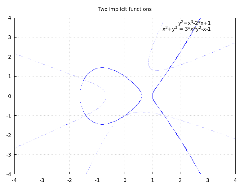
3D
implicit (fcn,x,xmin,xmax, y,ymin,ymax, z,zmin,zmax)
plots the implicit surface defined by fcn, with variable x taking values
from xmin to xmax, variable y taking values
from ymin to ymax and variable z taking values
from zmin to zmax. This object implements the marching cubes algorithm.
This object is affected by the following graphic options: x_voxel,
y_voxel, z_voxel, line_width, line_type, key,
wired_surface, enhanced3d and color.
Example:
(%i1) draw3d(
color=blue,
implicit((x^2+y^2+z^2-1)*(x^2+(y-1.5)^2+z^2-0.5)=0.015,
x,-1,1,y,-1.2,2.3,z,-1,1),
surface_hide=true);
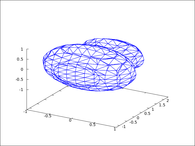
See also: ip_grid, ip_grid_in, line_width, line_type, key, x_voxel, y_voxel, z_voxel, wired_surface, enhanced3d.
interpolate_color — Variable
Default value: false
This option is relevant only when enhanced3d is not false.
When interpolate_color is false, surfaces are colored with
homogeneous quadrangles. When true, color transitions are smoothed
by interpolation.
interpolate_color also accepts a list of two numbers, [m,n].
For positive m and n, each quadrangle or triangle is interpolated
m times and n times in the respective direction. For negative
m and n, the interpolation frequency is chosen so that there will be at least
|m| and |n| points drawn; you can consider this as a special gridding function.
Zeros, i.e. interpolate_color=[0,0], will automatically choose an
optimal number of interpolated surface points.
Also, interpolate_color=true is equivalent to interpolate_color=[0,0].
Examples:
Color interpolation with explicit functions.
(%i1) draw3d(
enhanced3d = sin(x*y),
explicit(20*exp(-x^2-y^2)-10, x ,-3, 3, y, -3, 3)) $

(%i2) draw3d(
interpolate_color = true,
enhanced3d = sin(x*y),
explicit(20*exp(-x^2-y^2)-10, x ,-3, 3, y, -3, 3)) $

(%i3) draw3d(
interpolate_color = [-10,0],
enhanced3d = sin(x*y),
explicit(20*exp(-x^2-y^2)-10, x ,-3, 3, y, -3, 3)) $
Color interpolation with the mesh graphic object.
Interpolating colors in parametric surfaces can give unexpected results.
(%i1) draw3d(
enhanced3d = true,
mesh([[1,1,3], [7,3,1],[12,-2,4],[15,0,5]],
[[2,7,8], [4,3,1],[10,5,8], [12,7,1]],
[[-2,11,10],[6,9,5],[6,15,1], [20,15,2]])) $
(%i2) draw3d(
enhanced3d = true,
interpolate_color = true,
mesh([[1,1,3], [7,3,1],[12,-2,4],[15,0,5]],
[[2,7,8], [4,3,1],[10,5,8], [12,7,1]],
[[-2,11,10],[6,9,5],[6,15,1], [20,15,2]])) $
(%i3) draw3d(
enhanced3d = true,
interpolate_color = true,
view=map,
mesh([[1,1,3], [7,3,1],[12,-2,4],[15,0,5]],
[[2,7,8], [4,3,1],[10,5,8], [12,7,1]],
[[-2,11,10],[6,9,5],[6,15,1], [20,15,2]])) $
See also enhanced3d.
See also: enhanced3d.
ip_grid — Variable
Default value: [50, 50]
ip_grid sets the grid for the first sampling in implicit plots.
This option is relevant only for implicit objects.
ip_grid_in — Variable
Default value: [5, 5]
ip_grid_in sets the grid for the second sampling in implicit plots.
This option is relevant only for implicit objects.
key — Variable
Default value: "" (empty string)
key is the name of a function in the legend. If key is an
empty string, no key is assigned to the function.
This option affects the following graphic objects:
gr2d: points, polygon, rectangle,
ellipse, vector, explicit, implicit,
parametric and polar.
gr3d: points, explicit, parametric
and parametric_005fsurface.
Example:
(%i1) draw2d(key = "Sinus",
explicit(sin(x),x,0,10),
key = "Cosinus",
color = red,
explicit(cos(x),x,0,10) )$
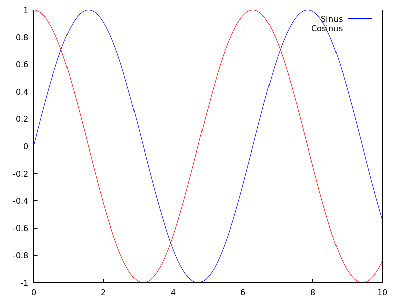
See also: points, polygon, rectangle, ellipse, vector, explicit, implicit, parametric, polar, parametric_surface.
key_pos — Variable
Default value: "" (empty string)
key_pos defines at which position the legend will be drawn. If key is an
empty string, "top_right" is used.
Available position specifiers are: top_left, top_center, top_right,
center_left, center, center_right,
bottom_left, bottom_center, and bottom_right.
Since this is a global graphics option, its position in the scene description does not matter.
Example:
(%i1) draw2d(
key_pos = top_left,
key = "x",
explicit(x, x,0,10),
color= red,
key = "x squared",
explicit(x^2,x,0,10))$
(%i3) draw3d(
key_pos = center,
key = "x",
explicit(x+y,x,0,10,y,0,10),
color= red,
key = "x squared",
explicit(x^2+y^2,x,0,10,y,0,10))$
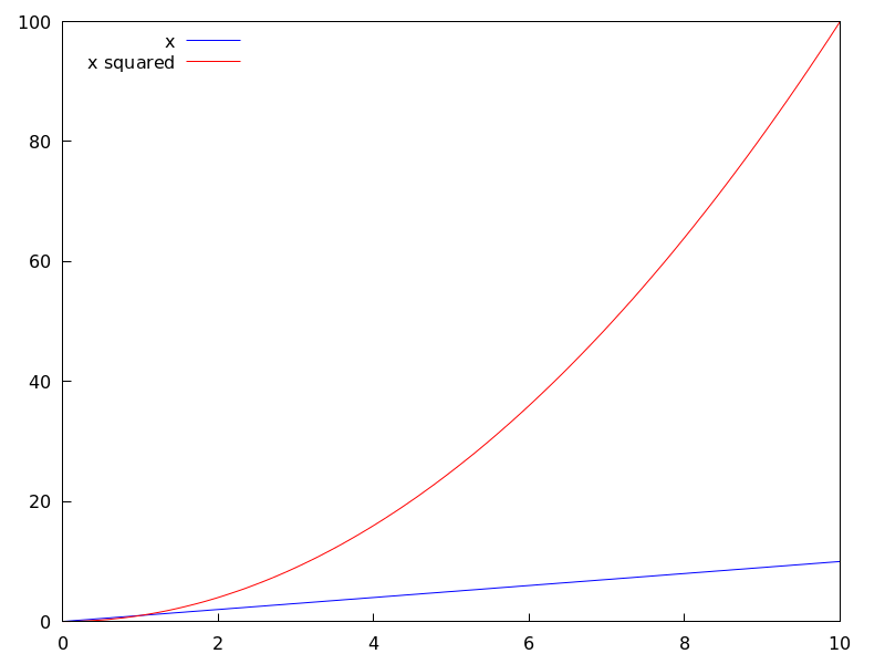
label_alignment — Variable
Default value: center
label_alignment is used to specify where to write labels with
respect to the given coordinates. Possible values are: center,
left, and right.
This option is relevant only for label objects.
Example:
(%i1) draw2d(xrange = [0,10],
yrange = [0,10],
points_joined = true,
points([[5,0],[5,10]]),
color = blue,
label(["Centered alignment (default)",5,2]),
label_alignment = 'left,
label(["Left alignment",5,5]),
label_alignment = 'right,
label(["Right alignment",5,8]))$
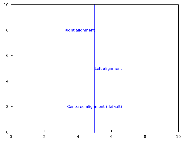
See also label_orientation, and color
See also: label_orientation.
label_orientation — Variable
Default value: horizontal
label_orientation is used to specify orientation of labels.
Possible values are: horizontal, and vertical.
This option is relevant only for label objects.
Example:
In this example, a dummy point is added to get an image.
Package draw needs always data to draw an scene.
(%i1) draw2d(xrange = [0,10],
yrange = [0,10],
point_size = 0,
points([[5,5]]),
color = navy,
label(["Horizontal orientation (default)",5,2]),
label_orientation = 'vertical,
color = "#654321",
label(["Vertical orientation",1,5]))$
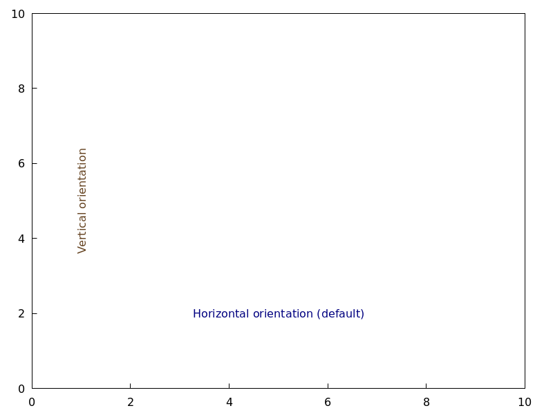
See also label_alignment and color
See also: label_alignment.
line_type — Variable
Default value: solid
line_type indicates how lines are displayed; possible values are
solid and dots, both available in all terminals, and
dashes, short_dashes, short_long_dashes, short_short_long_dashes,
and dot_dash, which are not available in png, jpg, and gif terminals.
This option affects the following graphic objects:
gr2d: points, polygon, rectangle,
ellipse, vector, explicit, implicit,
parametric and polar.
gr3d: points, explicit, parametric and parametric_005fsurface.
Example:
(%i1) draw2d(line_type = dots,
explicit(1 + x^2,x,-1,1),
line_type = solid, /* default */
explicit(2 + x^2,x,-1,1))$
See also line_005fwidth.
See also: points, polygon, rectangle, ellipse, vector, explicit, implicit, parametric, polar, parametric_surface, line_width.
line_width — Variable
Default value: 1
line_width is the width of plotted lines.
Its value must be a positive number.
This option affects the following graphic objects:
gr2d: points, polygon, rectangle,
ellipse, vector, explicit, implicit,
parametric and polar.
gr3d: points and parametric.
Example:
(%i1) draw2d(explicit(x^2,x,-1,1), /* default width */
line_width = 5.5,
explicit(1 + x^2,x,-1,1),
line_width = 10,
explicit(2 + x^2,x,-1,1))$
See also line_005ftype.
See also: points, polygon, rectangle, ellipse, vector, explicit, implicit, parametric, polar, line_type.
logcb — Variable
Default value: false
If logcb is true, the tics in the colorbox will be drawn in the
logarithmic scale.
When enhanced3d or colorbox is false, option logcb has
no effect.
Since this is a global graphics option, its position in the scene description does not matter.
Example:
(%i1) draw3d (
enhanced3d = true,
color = green,
logcb = true,
logz = true,
palette = [-15,24,-9],
explicit(exp(x^2-y^2), x,-2,2,y,-2,2)) $
See also enhanced3d, colorbox and cbrange.
See also: logcb, enhanced3d, colorbox, cbrange.
logx_secondary — Variable
Default value: false
If logx_secondary is true, the secondary x axis
will be drawn in the logarithmic scale.
This option is relevant only for 2d scenes.
Since this is a global graphics option, its position in the scene description does not matter.
Example:
(%i1) draw2d(
grid = true,
key="x^2, linear scale",
color=red,
explicit(x^2,x,1,100),
xaxis_secondary = true,
xtics_secondary = true,
logx_secondary = true,
key = "x^2, logarithmic x scale",
color = blue,
explicit(x^2,x,1,100) )$
See also logx_draw, logy_draw, logy_secondary, and logz.
See also: logx_draw, logy_draw, logy_secondary, logz.
logy_secondary — Variable
Default value: false
If logy_secondary is true, the secondary y axis
will be drawn in the logarithmic scale.
This option is relevant only for 2d scenes.
Since this is a global graphics option, its position in the scene description does not matter.
Example:
(%i1) draw2d(
grid = true,
key="x^2, linear scale",
color=red,
explicit(x^2,x,1,100),
yaxis_secondary = true,
ytics_secondary = true,
logy_secondary = true,
key = "x^2, logarithmic y scale",
color = blue,
explicit(x^2,x,1,100) )$
See also logx_draw, logy_draw, logx_secondary, and logz.
See also: logx_draw, logy_draw, logx_secondary, logz.
logz — Variable
Default value: false
If logz is true, the z axis will be drawn in the
logarithmic scale.
Since this is a global graphics option, its position in the scene description does not matter.
Example:
(%i1) draw3d(logz = true,
explicit(exp(u^2+v^2),u,-2,2,v,-2,2))$
See also logx_draw and logy_005fdraw.
See also: logx_draw, logy_draw.
make_level_picture (data) — Function
Returns a levels picture object. make_level_picture (data)
builds the picture object from matrix data.
make_level_picture (data,width,height)
builds the object from a list of numbers; in this case, both the
width and the height must be given.
The returned picture object contains the following four parts:
- symbol
level - image width
- image height
- an integer array with pixel data ranging from 0 to 255. Argument data must contain only numbers ranged from 0 to 255; negative numbers are substituted by 0, and those which are greater than 255 are set to 255.
Example:
Level picture from matrix.
(%i1) make_level_picture(matrix([3,2,5],[7,-9,3000]));
(%o1) picture(level, 3, 2, {Array: #(3 2 5 7 0 255)})
Level picture from numeric list.
(%i1) make_level_picture([-2,0,54,%pi],2,2);
(%o1) picture(level, 2, 2, {Array: #(0 0 54 3)})
make_poly_continent (continent_name) — Function
Makes the necessary polygons to draw a colored continent or a list of countries.
Example:
(%i1) load("worldmap")$
(%i2) /* A continent */
make_poly_continent(Africa)$
(%i3) apply(draw2d, %)$
(%i4) /* A list of countries */
make_poly_continent([Germany,Denmark,Poland])$
(%i5) apply(draw2d, %)$
make_poly_country (country_name) — Function
Makes the necessary polygons to draw a colored country. If islands exist, one country can be defined with more than just one polygon.
Example:
(%i1) load("worldmap")$
(%i2) make_poly_country(India)$
(%i3) apply(draw2d, %)$
make_polygon (nlist) — Function
Returns a polygon object from boundary indices. Argument
nlist is a list of components of boundaries_array.
Example:
Bhutan is defined by boundary numbers 171, 173
and 1143, so that make_polygon([171,173,1143])
appends arrays of coordinates boundaries_array[171],
boundaries_array[173] and boundaries_array[1143] and
returns a polygon object suited to be plotted by
draw. To avoid an error message, arrays must be
compatible in the sense that any two consecutive
arrays have two coordinates in the extremes in common. In this
example, the two first components of boundaries_array[171] are
equal to the last two coordinates of boundaries_array[173], and
the two first of boundaries_array[173] are equal to the two first
of boundaries_array[1143]; in conclusion, boundary numbers
171, 173 and 1143 (in this order) are compatible and the colored
polygon can be drawn.
(%i1) load("worldmap")$
(%i2) Bhutan;
(%o2) [[171, 173, 1143]]
(%i3) boundaries_array[171];
(%o3) {Array:
#(88.750549 27.14727 88.806351 27.25305 88.901367 27.282221
88.917877 27.321039)}
(%i4) boundaries_array[173];
(%o4) {Array:
#(91.659554 27.76511 91.6008 27.66666 91.598022 27.62499
91.631348 27.536381 91.765533 27.45694 91.775253 27.4161
92.007751 27.471939 92.11441 27.28583 92.015259 27.168051
92.015533 27.08083 92.083313 27.02277 92.112183 26.920271
92.069977 26.86194 91.997192 26.85194 91.915253 26.893881
91.916924 26.85416 91.8358 26.863331 91.712479 26.799999
91.542191 26.80444 91.492188 26.87472 91.418854 26.873329
91.371353 26.800831 91.307457 26.778049 90.682457 26.77417
90.392197 26.903601 90.344131 26.894159 90.143044 26.75333
89.98996 26.73583 89.841919 26.70138 89.618301 26.72694
89.636093 26.771111 89.360786 26.859989 89.22081 26.81472
89.110237 26.829161 88.921631 26.98777 88.873016 26.95499
88.867737 27.080549 88.843307 27.108601 88.750549
27.14727)}
(%i5) boundaries_array[1143];
(%o5) {Array:
#(91.659554 27.76511 91.666924 27.88888 91.65831 27.94805
91.338028 28.05249 91.314972 28.096661 91.108856 27.971109
91.015808 27.97777 90.896927 28.05055 90.382462 28.07972
90.396088 28.23555 90.366074 28.257771 89.996353 28.32333
89.83165 28.24888 89.58609 28.139999 89.35997 27.87166
89.225517 27.795 89.125793 27.56749 88.971077 27.47361
88.917877 27.321039)}
(%i6) Bhutan_polygon: make_polygon([171,173,1143])$
(%i7) draw2d(Bhutan_polygon)$
make_rgb_picture (redlevel, greenlevel, bluelevel) — Function
Returns an rgb-coloured picture object. All three arguments must be levels picture; with red, green and blue levels.
The returned picture object contains the following four parts:
- symbol
rgb - image width
- image height
- an integer array of length 3widthheight with pixel data ranging from 0 to 255. Each pixel is represented by three consecutive numbers (red, green, blue).
Example:
(%i1) red: make_level_picture(matrix([3,2],[7,260]));
(%o1) picture(level, 2, 2, {Array: #(3 2 7 255)})
(%i2) green: make_level_picture(matrix([54,23],[73,-9]));
(%o2) picture(level, 2, 2, {Array: #(54 23 73 0)})
(%i3) blue: make_level_picture(matrix([123,82],[45,32.5698]));
(%o3) picture(level, 2, 2, {Array: #(123 82 45 33)})
(%i4) make_rgb_picture(red,green,blue);
(%o4) picture(rgb, 2, 2,
{Array: #(3 54 123 2 23 82 7 73 45 255 0 33)})
mesh (row_1, row_2, …) — Function
Draws a quadrangular mesh in 3D.
3D
Argument row_i is a list of n 3D points of the form
[[x_i1,y_i1,z_i1], ...,[x_in,y_in,z_in]], and all rows are
of equal length. All these points define an arbitrary surface in 3D and
in some sense it’s a generalization of the elevation_grid object.
This object is affected by the following graphic options: line_type,
line_width, color, key, wired_surface, enhanced3d and transform.
Examples:
A simple example.
(%i1) draw3d(
mesh([[1,1,3], [7,3,1],[12,-2,4],[15,0,5]],
[[2,7,8], [4,3,1],[10,5,8], [12,7,1]],
[[-2,11,10],[6,9,5],[6,15,1], [20,15,2]])) $
Plotting a triangle in 3D.
(%i1) draw3d(
line_width = 2,
mesh([[1,0,0],[0,1,0]],
[[0,0,1],[0,0,1]])) $
Two quadrilaterals.
(%i1) draw3d(
surface_hide = true,
line_width = 3,
color = red,
mesh([[0,0,0], [0,1,0]],
[[2,0,2], [2,2,2]]),
color = blue,
mesh([[0,0,2], [0,1,2]],
[[2,0,4], [2,2,4]])) $
See also: line_type, line_width, color, key, wired_surface, enhanced3d, transform.
multiplot_mode (term) — Function
This function enables Maxima to work in one-window multiplot mode with terminal
term; accepted arguments for this function are screen,
wxt, aquaterm, windows and none.
When multiplot mode is enabled, each call to draw sends a new plot to the
same window, without erasing the previous ones. To disable the multiplot mode,
write multiplot_mode(none).
When multiplot mode is enabled, global option terminal is blocked and you
have to disable this working mode before changing to another terminal.
On Windows this feature requires Gnuplot 5.0 or newer.
Note, that just plotting multiple expressions into the same plot doesn’t require
multiplot: It can be done by just issuing multiple explicit or similar
commands in a row.
Example:
(%i1) set_draw_defaults(
xrange = [-1,1],
yrange = [-1,1],
grid = true,
title = "Step by step plot" )$
(%i2) multiplot_mode(screen)$
(%i3) draw2d(color=blue, explicit(x^2,x,-1,1))$
(%i4) draw2d(color=red, explicit(x^3,x,-1,1))$
(%i5) draw2d(color=brown, explicit(x^4,x,-1,1))$
(%i6) multiplot_mode(none)$
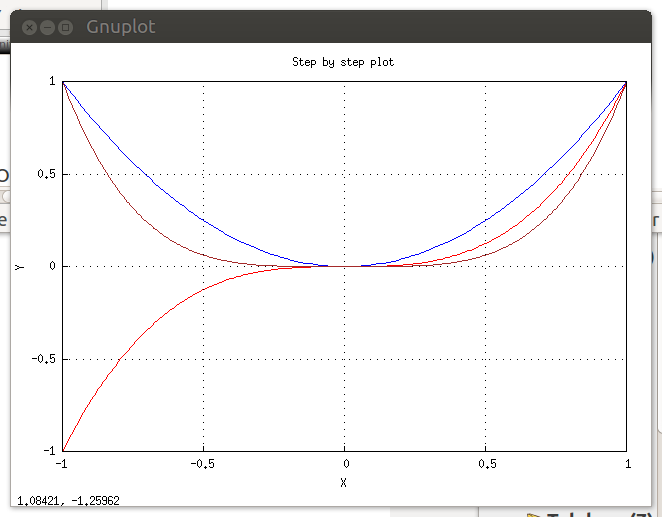
See also: explicit.
negative_picture (pic) — Function
Returns the negative of a (level or rgb) picture.
numbered_boundaries (nlist) — Function
Draws a list of polygonal segments (boundaries), labeled by
its numbers (boundaries_array coordinates). This is of great
help when building new geographical entities.
Example:
Map of Europe labeling borders with their component number in
boundaries_array.
(%i1) load("worldmap")$
(%i2) european_borders:
region_boundaries(-31.81,74.92,49.84,32.06)$
(%i3) numbered_boundaries(european_borders)$
parametric (xfun, yfun, par, parmin, parmax) — Function
Draws parametric functions in 2D and 3D.
This object is affected by the following graphic options: nticks,
line_width, line_type, key, color and enhanced3d.
2D
The command parametric(xfun, yfun, par, parmin, parmax) plots the parametric function [xfun, yfun],
with parameter par taking values from parmin to parmax.
Example:
(%i1) draw2d(explicit(exp(x),x,-1,3),
color = red,
key = "This is the parametric one!!",
parametric(2*cos(rrr),rrr^2,rrr,0,2*%pi))$
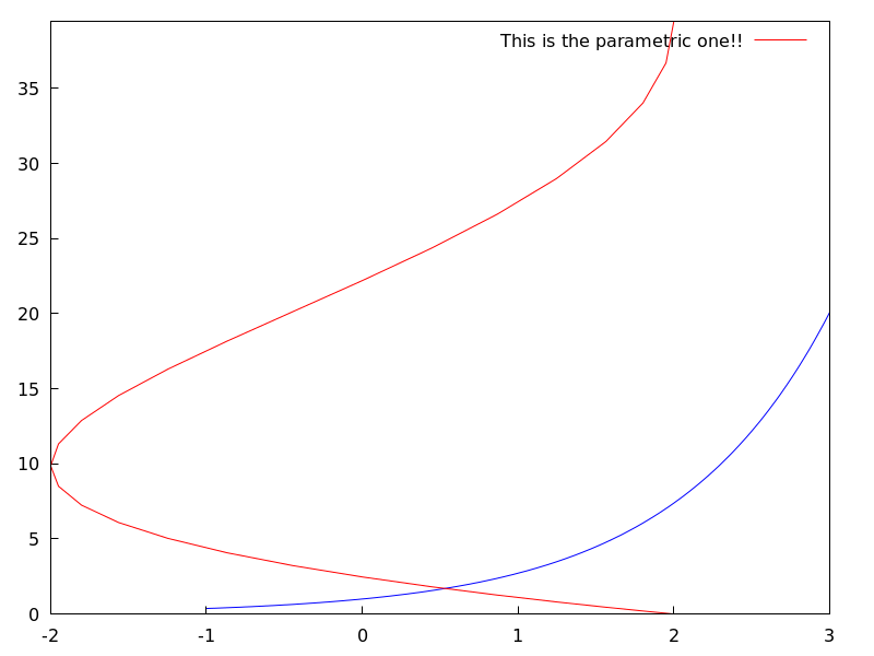
3D
parametric(xfun, yfun, zfun, par, parmin, parmax) plots the parametric curve [xfun, yfun, zfun], with parameter par taking values from parmin to
parmax.
Example:
(%i1) draw3d(explicit(exp(sin(x)+cos(x^2)),x,-3,3,y,-3,3),
color = royalblue,
parametric(cos(5*u)^2,sin(7*u),u-2,u,0,2),
color = turquoise,
line_width = 2,
parametric(t^2,sin(t),2+t,t,0,2),
surface_hide = true,
title = "Surface & curves" )$
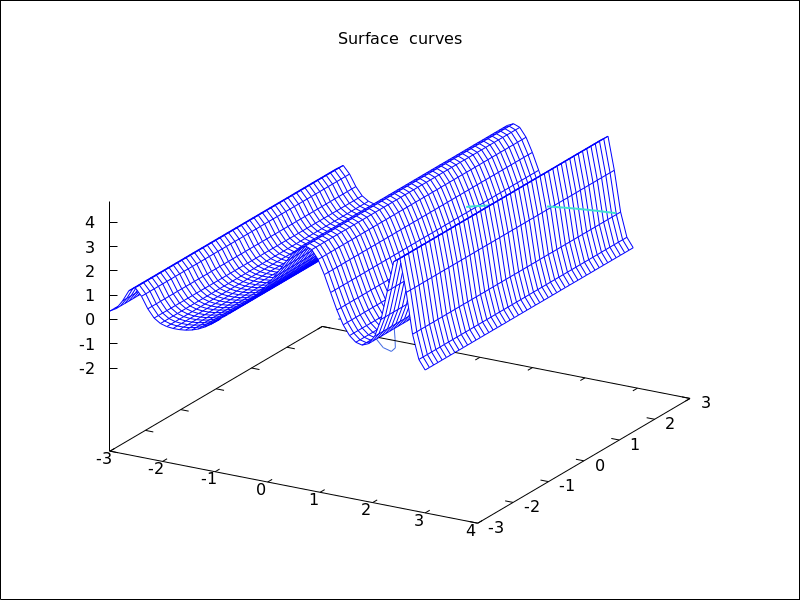
See also: nticks, line_width, line_type, key, color, enhanced3d.
parametric_surface (xfun, yfun, zfun, par1, par1min, par1max, par2, par2min, par2max) — Function
Draws parametric surfaces in 3D.
3D
The command parametric_surface(xfun, yfun, zfun, par1, par1min, par1max, par2, par2min, par2max) plots the parametric surface [xfun, yfun, zfun], with parameter par1 taking values from par1min to
par1max and parameter par2 taking values from par2min to
par2max.
This object is affected by the following graphic options: draw_realpart, xu_grid,
yv_grid, line_type, line_width, key, wired_surface, enhanced3d
and color.
Example:
(%i1) draw3d(title = "Sea shell",
xu_grid = 100,
yv_grid = 25,
view = [100,20],
surface_hide = true,
parametric_surface(0.5*u*cos(u)*(cos(v)+1),
0.5*u*sin(u)*(cos(v)+1),
u*sin(v) - ((u+3)/8*%pi)^2 - 20,
u, 0, 13*%pi, v, -%pi, %pi) )$
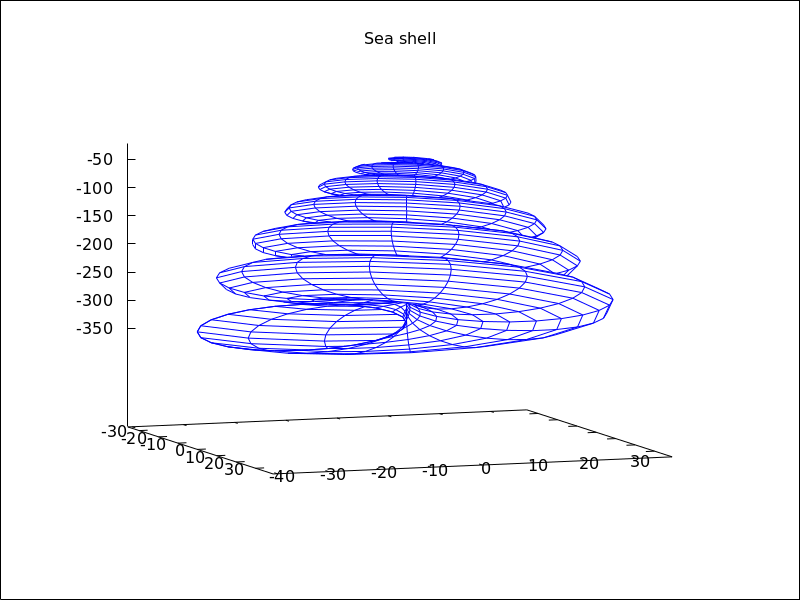
See also: draw_realpart, xu_grid, yv_grid, line_type, line_width, key, wired_surface, enhanced3d.
picture_equalp (x, y) — Function
Returns true in case of equal pictures, and false otherwise.
picturep (x) — Function
Returns true if the argument is a well formed image,
and false otherwise.
point_size — Variable
Default value: 1
point_size sets the size for plotted points. It must be a
non negative number.
This option has no effect when graphic option point_type is
set to dot.
This option affects the following graphic objects:
gr2d: points.
gr3d: points.
Example:
(%i1) draw2d(points(makelist([random(20),random(50)],k,1,10)),
point_size = 5,
points(makelist(k,k,1,20),makelist(random(30),k,1,20)))$
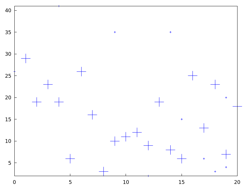
See also: points.
points ([[x1, y1], [x2, y2], …]) — Function
Draws points in 2D and 3D.
This object is affected by the following graphic options: point_size,
point_type, points_joined, line_width, key,
line_type and color. In 3D mode, it is also affected by enhanced3d
2D
points ([[x1,y1], [x2,y2],...]) or
points ([x1,x2,...], [y1,y2,...])
plots points [x1,y1], [x2,y2], etc. If abscissas
are not given, they are set to consecutive positive integers, so that
points ([y1,y2,...]) draws points [1,y1], [2,y2], etc.
If matrix is a two-column or two-row matrix, points (matrix)
draws the associated points. If matrix is an one-column or one-row matrix,
abscissas are assigned automatically.
If 1d_y_array is a 1D lisp array of numbers, points (1d_y_array) plots them
setting abscissas to consecutive positive integers. points (1d_x_array, 1d_y_array)
plots points with their coordinates taken from the two arrays passed as arguments. If
2d_xy_array is a 2D array with two columns, or with two rows, points (2d_xy_array)
plots the corresponding points on the plane.
Examples:
Two types of arguments for points, a list of pairs and two lists
of separate coordinates.
(%i1) draw2d(
key = "Small points",
points(makelist([random(20),random(50)],k,1,10)),
point_type = circle,
point_size = 3,
points_joined = true,
key = "Great points",
points(makelist(k,k,1,20),makelist(random(30),k,1,20)),
point_type = filled_down_triangle,
key = "Automatic abscissas",
color = red,
points([2,12,8]))$
Drawing impulses.
(%i1) draw2d(
points_joined = impulses,
line_width = 2,
color = red,
points(makelist([random(20),random(50)],k,1,10)))$
Array with ordinates.
(%i1) a: make_array (flonum, 100) $
(%i2) for i:0 thru 99 do a[i]: random(1.0) $
(%i3) draw2d(points(a)) $
Two arrays with separate coordinates.
(%i1) x: make_array (flonum, 100) $
(%i2) y: make_array (fixnum, 100) $
(%i3) for i:0 thru 99 do (
x[i]: float(i/100),
y[i]: random(10) ) $
(%i4) draw2d(points(x, y)) $
A two-column 2D array.
(%i1) xy: make_array(flonum, 100, 2) $
(%i2) for i:0 thru 99 do (
xy[i, 0]: float(i/100),
xy[i, 1]: random(10) ) $
(%i3) draw2d(points(xy)) $

Drawing an array filled with function read_array.
(%i1) a: make_array(flonum,100) $
(%i2) read_array (file_search ("pidigits.data"), a) $
(%i3) draw2d(points(a)) $
3D
points([[x1, y1, z1], [x2, y2, z2], ...]) or points([x1, x2, ...], [y1, y2, ...], [z1, z2,...]) plots points [x1, y1, z1],
[x2, y2, z2], etc. If matrix is a three-column
or three-row matrix, points (matrix) draws the associated points.
When arguments are lisp arrays, points (1d_x_array, 1d_y_array, 1d_z_array)
takes coordinates from the three 1D arrays. If 2d_xyz_array is a 2D array with three columns,
or with three rows, points (2d_xyz_array) plots the corresponding points.
Examples:
One tridimensional sample,
(%i1) load ("numericalio")$
(%i2) s2 : read_matrix (file_search ("wind.data"))$
(%i3) draw3d(title = "Daily average wind speeds",
point_size = 2,
points(args(submatrix (s2, 4, 5))) )$
Two tridimensional samples,
(%i1) load ("numericalio")$
(%i2) s2 : read_matrix (file_search ("wind.data"))$
(%i3) draw3d(
title = "Daily average wind speeds. Two data sets",
point_size = 2,
key = "Sample from stations 1, 2 and 3",
points(args(submatrix (s2, 4, 5))),
point_type = 4,
key = "Sample from stations 1, 4 and 5",
points(args(submatrix (s2, 2, 3))) )$
Unidimensional arrays,
(%i1) x: make_array (fixnum, 10) $
(%i2) y: make_array (fixnum, 10) $
(%i3) z: make_array (fixnum, 10) $
(%i4) for i:0 thru 9 do (
x[i]: random(10),
y[i]: random(10),
z[i]: random(10) ) $
(%i5) draw3d(points(x,y,z)) $
Bidimensional colored array,
(%i1) xyz: make_array(fixnum, 10, 3) $
(%i2) for i:0 thru 9 do (
xyz[i, 0]: random(10),
xyz[i, 1]: random(10),
xyz[i, 2]: random(10) ) $
(%i3) draw3d(
enhanced3d = true,
points_joined = true,
points(xyz)) $
Color numbers explicitly specified by the user.
(%i1) pts: makelist([t,t^2,cos(t)], t, 0, 15)$
(%i2) col_num: makelist(k, k, 1, length(pts))$
(%i3) draw3d(
enhanced3d = ['part(col_num,k),k],
point_size = 3,
point_type = filled_circle,
points(pts))$
See also: point_size, point_type, points_joined, line_width, key, line_type, enhanced3d.
points_joined — Variable
Default value: false
When points_joined is true, points are joined by lines; when false,
isolated points are drawn. A third possible value for this graphic option is
impulses; in such case, vertical segments are drawn from points to the x-axis (2D)
or to the xy-plane (3D).
This option affects the following graphic objects:
gr2d: points.
gr3d: points.
Example:
(%i1) draw2d(xrange = [0,10],
yrange = [0,4],
point_size = 3,
point_type = up_triangle,
color = blue,
points([[1,1],[5,1],[9,1]]),
points_joined = true,
point_type = square,
line_type = dots,
points([[1,2],[5,2],[9,2]]),
point_type = circle,
color = red,
line_width = 7,
points([[1,3],[5,3],[9,3]]) )$
See also: points.
polar (radius, ang, minang, maxang) — Function
Draws 2D functions defined in polar coordinates.
2D
polar (radius,ang,minang,maxang) plots function
radius(ang) defined in polar coordinates, with variable
ang taking values from
minang to maxang.
This object is affected by the following graphic options: nticks,
line_width, line_type, key and color.
Example:
(%i1) draw2d(user_preamble = "set grid polar",
nticks = 200,
xrange = [-5,5],
yrange = [-5,5],
color = blue,
line_width = 3,
title = "Hyperbolic Spiral",
polar(10/theta,theta,1,10*%pi) )$
See also: nticks, line_width, line_type, key.
polygon ([[x1, y1], [x2, y2], …]) — Function
Draws polygons in 2D.
2D
The commands polygon([[x1, y1], [x2, y2], ...])
or polygon([x1, x2, ...], [y1, y2, ...]) plot on
the plane a polygon with vertices [x1, y1], [x2, y2], etc.
This object is affected by the following graphic options: transparent,
fill_color, fill_density, border, line_width, key,
line_type and color.
Example:
(%i1) draw2d(color = "#e245f0",
line_width = 8,
polygon([[3,2],[7,2],[5,5]]),
border = false,
fill_color = yellow,
polygon([[5,2],[9,2],[7,5]]) )$
See also: transparent, fill_color, fill_density, border, line_width, key, line_type.
proportional_axes — Variable
Default value: none
When proportional_axes is equal to xy or xyz,
the aspect ratio of the axis units will be set to 1:1 resulting in a 2D or 3D
scene that will be drawn with axes proportional to their relative lengths.
Since this is a global graphics option, its position in the scene description does not matter.
This option works with Gnuplot version 4.2.6 or greater.
Examples:
Single 2D plot.
(%i1) draw2d(
ellipse(0,0,1,1,0,360),
transparent=true,
color = blue,
line_width = 4,
ellipse(0,0,2,1/2,0,360),
proportional_axes = 'xy) $
Multiplot.
(%i1) draw(
terminal = wxt,
gr2d(proportional_axes = 'xy,
explicit(x^2,x,0,1)),
gr2d(explicit(x^2,x,0,1),
xrange = [0,1],
yrange = [0,2],
proportional_axes='xy),
gr2d(explicit(x^2,x,0,1)))$
quadrilateral (point_1, point_2, point_3, point_4) — Function
Draws a quadrilateral.
2D
quadrilateral([x1, y1], [x2, y2], [x3, y3], [x4, y4]) draws a quadrilateral with vertices
[x1, y1], [x2, y2],
[x3, y3], and [x4, y4].
This object is affected by the following graphic options:
transparent, fill_color, border, line_width,
key, xaxis_secondary, yaxis_secondary, line_type,
transform and color.
Example:
(%i1) draw2d(
quadrilateral([1,1],[2,2],[3,-1],[2,-2]))$
3D
quadrilateral([x1, y1, z1], [x2, y2, z2], [x3, y3, z3], [x4, y4, z4])
draws a quadrilateral with vertices [x1, y1, z1],
[x2, y2, z2], [x3, y3, z3],
and [x4, y4, z4].
This object is affected by the following graphic options: line_type,
line_width, color, key, enhanced3d and
transform.
See also: transparent, fill_color, border, line_width, key, xaxis_secondary, yaxis_secondary, line_type, color, enhanced3d, transform.
read_xpm (xpm_file) — Function
Reads a file in xpm and returns a picture object.
rectangle ([x1, y1], [x2, y2]) — Function
Draws rectangles in 2D.
2D
rectangle ([x1,y1], [x2,y2]) draws a rectangle with opposite vertices
[x1,y1] and [x2,y2].
This object is affected by the following graphic options: transparent,
fill_color, border, line_width, key,
line_type and color.
Example:
(%i1) draw2d(fill_color = red,
line_width = 6,
line_type = dots,
transparent = false,
fill_color = blue,
rectangle([-2,-2],[8,-1]), /* opposite vertices */
transparent = true,
line_type = solid,
line_width = 1,
rectangle([9,4],[2,-1.5]),
xrange = [-3,10],
yrange = [-3,4.5] )$
See also: transparent, fill_color, border, line_width, key, line_type.
region (expr, var1, minval1, maxval1, var2, minval2, maxval2) — Function
Plots a region on the plane defined by inequalities.
2D
expr is an expression formed by inequalities and boolean operators
and, or, and not. The region is bounded by the rectangle
defined by $[minval1, maxval1]$ and $[minval2, maxval2]$.
This object is affected by the following graphic options: fill_color, fill_density,
key, x_voxel and y_005fvoxel.
Example:
(%i1) draw2d(
x_voxel = 30,
y_voxel = 30,
region(x^2+y^2<1 and x^2+y^2 > 1/2,
x, -1.5, 1.5, y, -1.5, 1.5));
See also: not, fill_color, fill_density, key, x_voxel, y_voxel.
region_boundaries (x1, y1, x2, y2) — Function
Detects polygonal segments of global variable boundaries_array
fully contained in the rectangle with vertices (x1,y1) -upper left-
and (x2,y2) -bottom right-.
Example:
Returns segment numbers for plotting southern Italy.
(%i1) load("worldmap")$
(%i2) region_boundaries(10.4,41.5,20.7,35.4);
(%o2) [1846, 1863, 1864, 1881, 1888, 1894]
(%i3) draw2d(geomap(%))$
region_boundaries_plus (x1, y1, x2, y2) — Function
Detects polygonal segments of global variable boundaries_array
containing at least one vertex in the rectangle defined by vertices (x1,y1)
-upper left- and (x2,y2) -bottom right-.
Example:
(%i1) load("worldmap")$
(%i2) region_boundaries_plus(10.4,41.5,20.7,35.4);
(%o2) [1060, 1062, 1076, 1835, 1839, 1844, 1846, 1858,
1861, 1863, 1864, 1871, 1881, 1888, 1894, 1897]
(%i3) draw2d(geomap(%))$
rgb2level (pic) — Function
Transforms an rgb picture into a level one by averaging the red, green and blue channels.
set_draw_defaults (graphic option, …, graphic object, …) — Function
Sets user graphics options. This function is useful for plotting a sequence of graphics with common graphics options. Calling this function without arguments removes user defaults.
Example:
(%i1) set_draw_defaults(
xrange = [-10,10],
yrange = [-2, 2],
color = blue,
grid = true)$
(%i2) /* plot with user defaults */
draw2d(explicit(((1+x)**2/(1+x*x))-1,x,-10,10))$
(%i3) set_draw_defaults()$
(%i4) /* plot with standard defaults */
draw2d(explicit(((1+x)**2/(1+x*x))-1,x,-10,10))$
spherical (radius, azi, minazi, maxazi, zen, minzen, maxzen) — Function
Draws 3D functions defined in spherical coordinates.
3D
spherical(radius, azi, minazi, maxazi, zen, minzen, maxzen) plots the function radius(azi, zen) defined in spherical coordinates, with azimuth azi taking
values from minazi to maxazi and zenith zen taking values
from minzen to maxzen.
This object is affected by the following graphic options: xu_grid,
yv_grid, line_type, key, wired_surface, enhanced3d and color.
Example:
(%i1) draw3d(spherical(1,a,0,2*%pi,z,0,%pi))$
See also: xu_grid, yv_grid, line_type, key, wired_surface, enhanced3d.
surface_hide — Variable
Default value: false
If surface_hide is true, hidden parts are not plotted in 3d surfaces.
Since this is a global graphics option, its position in the scene description does not matter.
Example:
(%i1) draw(columns=2,
gr3d(explicit(exp(sin(x)+cos(x^2)),x,-3,3,y,-3,3)),
gr3d(surface_hide = true,
explicit(exp(sin(x)+cos(x^2)),x,-3,3,y,-3,3)) )$
take_channel (im, color) — Function
If argument color is red, green or blue,
function take_channel returns the corresponding color channel of
picture im.
Example:
(%i1) red: make_level_picture(matrix([3,2],[7,260]));
(%o1) picture(level, 2, 2, {Array: #(3 2 7 255)})
(%i2) green: make_level_picture(matrix([54,23],[73,-9]));
(%o2) picture(level, 2, 2, {Array: #(54 23 73 0)})
(%i3) blue: make_level_picture(matrix([123,82],[45,32.5698]));
(%o3) picture(level, 2, 2, {Array: #(123 82 45 33)})
(%i4) make_rgb_picture(red,green,blue);
(%o4) picture(rgb, 2, 2,
{Array: #(3 54 123 2 23 82 7 73 45 255 0 33)})
(%i5) take_channel(%,'green); /* simple quote!!! */
(%o5) picture(level, 2, 2, {Array: #(54 23 73 0)})
terminal — Variable
Default value: screen
Selects the terminal to be used by Gnuplot; possible values are:
screen (default), png, pngcairo, jpg, gif,
cairolatex_pdf, cairolatex_pdf_standalone,
eps, eps_color, epslatex, epslatex_standalone,
svg, canvas, dumb, dumb_file, pdf, pdfcairo,
wxt, animated_gif, multipage_pdfcairo, multipage_pdf,
multipage_eps, multipage_eps_color, tikz, tikz_standalone
and aquaterm.
Terminals screen, wxt, windows and aquaterm can
be also defined as a list
with two elements: the name of the terminal itself and a non negative integer number.
In this form, multiple windows can be opened at the same time, each with its
corresponding number. This feature does not work in Windows platforms.
Since this is a global graphics option, its position in the scene description
does not matter. It can be also used as an argument of function draw.
N.B. pdfcairo requires Gnuplot 4.3 or newer.
pdf requires Gnuplot to be compiled with the option --enable-pdf and libpdf must
be installed. The pdf library is available from: http://www.pdflib.com/en/download/pdflib-family/pdflib-lite/
Examples:
(%i1) /* screen terminal (default) */
draw2d(explicit(x^2,x,-1,1))$
(%i2) /* png file */
draw2d(terminal = 'png,
explicit(x^2,x,-1,1))$
(%i3) /* jpg file */
draw2d(terminal = 'jpg,
dimensions = [300,300],
explicit(x^2,x,-1,1))$
(%i4) /* eps file */
draw2d(file_name = "myfile",
explicit(x^2,x,-1,1),
terminal = 'eps)$
(%i5) /* pdf file */
draw2d(file_name = "mypdf",
dimensions = 100*[12.0,8.0],
explicit(x^2,x,-1,1),
terminal = 'pdf)$
(%i6) /* wxwidgets window */
draw2d(explicit(x^2,x,-1,1),
terminal = 'wxt)$
(%i7) /* tikz file */
draw2d(explicit(x^2,x,-1,1),
file_name = "mytikz",
dimensions = [8,8], /* in cms */
terminal = 'tikz)$
Multiple windows.
(%i1) draw2d(explicit(x^5,x,-2,2), terminal=[screen, 3])$
(%i2) draw2d(explicit(x^2,x,-2,2), terminal=[screen, 0])$
An animated gif file.
(%i1) draw(
delay = 100,
file_name = "zzz",
terminal = 'animated_gif,
gr2d(explicit(x^2,x,-1,1)),
gr2d(explicit(x^3,x,-1,1)),
gr2d(explicit(x^4,x,-1,1)));
End of animation sequence
(%o1) [gr2d(explicit), gr2d(explicit), gr2d(explicit)]
Option delay is only active in animated gif’s; it is ignored in
any other case.
Multipage output in eps format.
(%i1) draw(
file_name = "parabol",
terminal = multipage_eps,
dimensions = 100*[10,10],
gr2d(explicit(x^2,x,-1,1)),
gr3d(explicit(x^2+y^2,x,-1,1,y,-1,1))) $
See also file_name, dimensions_draw and delay.
See also: file_name, dimensions_draw, delay.
transform — Variable
Default value: none
If transform is none, the space is not transformed and
graphic objects are drawn as defined. When a space transformation is
desired, a list must be assigned to option transform. In case of
a 2D scene, the list takes the form [f1(x,y), f2(x,y), x, y].
In case of a 3D scene, the list is of the form
[f1(x,y,z), f2(x,y,z), f3(x,y,z), x, y, z].
The names of the variables defined in the lists may be different to those used in the definitions of the graphic objects.
Examples:
Rotation in 2D.
(%i1) th : %pi / 4$
(%i2) draw2d(
color = "#e245f0",
proportional_axes = 'xy,
line_width = 8,
triangle([3,2],[7,2],[5,5]),
border = false,
fill_color = yellow,
transform = [cos(th)*x - sin(th)*y,
sin(th)*x + cos(th)*y, x, y],
triangle([3,2],[7,2],[5,5]) )$
Translation in 3D.
(%i1) draw3d(
color = "#a02c00",
explicit(20*exp(-x^2-y^2)-10,x,-3,3,y,-3,3),
transform = [x+10,y+10,z+10,x,y,z],
color = blue,
explicit(20*exp(-x^2-y^2)-10,x,-3,3,y,-3,3) )$
transparent — Variable
Default value: false
If transparent is false, interior regions of polygons are
filled according to fill_color.
This option affects the following graphic objects:
gr2d: polygon, rectangle and ellipse.
Example:
(%i1) draw2d(polygon([[3,2],[7,2],[5,5]]),
transparent = true,
color = blue,
polygon([[5,2],[9,2],[7,5]]) )$
See also: polygon, rectangle, ellipse.
triangle (point_1, point_2, point_3) — Function
Draws a triangle.
2D
triangle ([x1,y1], [x2,y2], [x3,y3]) draws a triangle with vertices [x1,y1], [x2,y2],
and [x3,y3].
This object is affected by the following graphic options:
transparent, fill_color, border, line_width,
key, xaxis_secondary, yaxis_secondary, line_type,
transform and color.
Example:
(%i1) draw2d(
triangle([1,1],[2,2],[3,-1]))$
3D
triangle ([x1,y1,z1], [x2,y2,z2], [x3,y3,z3]) draws a triangle with vertices [x1,y1,z1],
[x2,y2,z2], and [x3,y3,z3].
This object is affected by the following graphic options: line_type,
line_width, color, key, enhanced3d and transform.
See also: transparent, fill_color, border, line_width, key, xaxis_secondary, yaxis_secondary, line_type, transform, color, enhanced3d.
tube (xfun, yfun, zfun, rfun, p, pmin, pmax) — Function
Draws a tube in 3D with varying diameter.
3D
[xfun,yfun,zfun]
is the parametric curve with parameter p taking values from pmin
to pmax. Circles of radius rfun are placed with their centers on
the parametric curve and perpendicular to it.
This object is affected by the following graphic options: xu_grid,
yv_grid, line_type, line_width, key, wired_surface, enhanced3d,
color and capping.
Example:
(%i1) draw3d(
enhanced3d = true,
xu_grid = 50,
tube(cos(a), a, 0, cos(a/10)^2,
a, 0, 4*%pi) )$
See also: xu_grid, yv_grid, line_type, line_width, key, wired_surface, enhanced3d, color, capping.
unit_vectors — Variable
Default value: false
If unit_vectors is true, vectors are plotted with module 1.
This is useful for plotting vector fields. If unit_vectors is false,
vectors are plotted with its original length.
This option is relevant only for vector objects.
Example:
(%i1) draw2d(xrange = [-1,6],
yrange = [-1,6],
head_length = 0.1,
vector([0,0],[5,2]),
unit_vectors = true,
color = red,
vector([0,3],[5,2]))$
user_preamble — Variable
Default value: "" (empty string)
Expert Gnuplot users can make use of this option to fine tune Gnuplot’s
behaviour by writing settings to be sent before the plot or splot
command.
The value of this option must be a string or a list of strings (one per line).
Since this is a global graphics option, its position in the scene description does not matter.
Example:
Tell Gnuplot to draw axes and grid on top of graphics objects,
(%i1) draw2d(
xaxis =true, xaxis_type=solid,
yaxis =true, yaxis_type=solid,
user_preamble="set grid front",
region(x^2+y^2<1 ,x,-1.5,1.5,y,-1.5,1.5))$
Tell gnuplot to draw all contour lines in black
(%i1) draw3d(
contour=both,
surface_hide=true,enhanced3d=true,wired_surface=true,
contour_levels=10,
user_preamble="set for [i=1:8] linetype i dashtype i linecolor 0",
explicit(sin(x)*cos(y),x,1,10,y,1,10)
);
vector ([x, y], [dx, dy]) — Function
Draws vectors in 2D and 3D.
This object is affected by the following graphic options: head_both,
head_length, head_angle, head_type, line_width,
line_type, key and color.
2D
vector([x,y], [dx,dy]) plots vector
[dx,dy] with origin in [x,y].
Example:
(%i1) draw2d(xrange = [0,12],
yrange = [0,10],
head_length = 1,
vector([0,1],[5,5]), /* default type */
head_type = 'empty,
vector([3,1],[5,5]),
head_both = true,
head_type = 'nofilled,
line_type = dots,
vector([6,1],[5,5]))$
3D
vector([x,y,z], [dx,dy,dz])
plots vector [dx,dy,dz] with
origin in [x,y,z].
Example:
(%i1) draw3d(color = cyan,
vector([0,0,0],[1,1,1]/sqrt(3)),
vector([0,0,0],[1,-1,0]/sqrt(2)),
vector([0,0,0],[1,1,-2]/sqrt(6)) )$
See also: head_both, head_length, head_angle, head_type, line_width, line_type, key.
view — Variable
Default value: [60,30]
A pair of angles, measured in degrees, indicating the view direction in a 3D scene. The first angle is the vertical rotation around the x axis, in the range $[0, 360]$. The second one is the horizontal rotation around the z axis, in the range $[0, 360]$.
If option view is given the value map, the view direction is set
to be perpendicular to the xy-plane.
Since this is a global graphics option, its position in the scene description does not matter.
Example:
(%i1) draw3d(view = [170, 50],
enhanced3d = true,
explicit(sin(x^2+y^2),x,-2,2,y,-2,2) )$
(%i2) draw3d(view = map,
enhanced3d = true,
explicit(sin(x^2+y^2),x,-2,2,y,-2,2) )$
wired_surface — Variable
Default value: false
Indicates whether 3D surfaces in enhanced3d mode show the grid joining
the points or not.
Since this is a global graphics option, its position in the scene description does not matter.
Example:
(%i1) draw3d(
enhanced3d = [sin(x),x,y],
wired_surface = true,
explicit(x^2+y^2,x,-1,1,y,-1,1)) $
x_voxel — Variable
Default value: 10
x_voxel is the number of voxels in the x direction to
be used by the marching cubes algorithm implemented
by the 3d implicit object. It is also used by graphic
object region.
See also: region.
xaxis — Variable
Default value: false
If xaxis is true, the x axis is drawn.
Since this is a global graphics option, its position in the scene description does not matter.
Example:
(%i1) draw2d(explicit(x^3,x,-1,1),
xaxis = true,
xaxis_color = blue)$
See also xaxis_width, xaxis_type and xaxis_005fcolor.
See also: xaxis_width, xaxis_type, xaxis_color.
xaxis_color — Variable
Default value: "black"
xaxis_color specifies the color for the x axis. See
color to know how colors are defined.
Since this is a global graphics option, its position in the scene description does not matter.
Example:
(%i1) draw2d(explicit(x^3,x,-1,1),
xaxis = true,
xaxis_color = red)$
See also xaxis, xaxis_width and xaxis_005ftype.
See also: xaxis, xaxis_width, xaxis_type.
xaxis_secondary — Variable
Default value: false
If xaxis_secondary is true, function values can be plotted with
respect to the second x axis, which will be drawn on top of the scene.
Note that this is a local graphics option which only affects to 2d plots.
Example:
(%i1) draw2d(
key = "Bottom x-axis",
explicit(x+1,x,1,2),
color = red,
key = "Above x-axis",
xtics_secondary = true,
xaxis_secondary = true,
explicit(x^2,x,-1,1)) $
See also xrange_secondary, xtics_secondary, xtics_rotate_secondary,
xtics_axis_secondary and xaxis_005fsecondary.
See also: xrange_secondary, xtics_secondary, xtics_rotate_secondary, xaxis_secondary.
xaxis_type — Variable
Default value: dots
xaxis_type indicates how the x axis is displayed;
possible values are solid and dots
Since this is a global graphics option, its position in the scene description does not matter.
Example:
(%i1) draw2d(explicit(x^3,x,-1,1),
xaxis = true,
xaxis_type = solid)$
See also xaxis, xaxis_width and xaxis_005fcolor.
See also: xaxis, xaxis_width, xaxis_color.
xaxis_width — Variable
Default value: 1
xaxis_width is the width of the x axis.
Its value must be a positive number.
Since this is a global graphics option, its position in the scene description does not matter.
Example:
(%i1) draw2d(explicit(x^3,x,-1,1),
xaxis = true,
xaxis_width = 3)$
See also xaxis, xaxis_type and xaxis_005fcolor.
See also: xaxis, xaxis_type, xaxis_color.
xlabel_secondary — Variable
Default value: "" (empty string)
Option xlabel_secondary, a string, is the label for the secondary x axis.
By default, no label is written.
Since this is a global graphics option, its position in the scene description does not matter.
Example:
(%i1) draw2d(
xaxis_secondary=true,yaxis_secondary=true,
xtics_secondary=true,ytics_secondary=true,
xlabel_secondary="t[s]",
ylabel_secondary="U[V]",
explicit(sin(t),t,0,10) )$
See also xlabel_draw, ylabel_draw, ylabel_secondary and zlabel_005fdraw.
See also: xlabel_draw, ylabel_draw, ylabel_secondary, zlabel_draw.
xrange — Variable
Default value: auto
If xrange is auto, the range for the x coordinate is
computed automatically.
If the user wants a specific interval for x, it must be given as a
Maxima list, as in xrange=[-2, 3].
Since this is a global graphics option, its position in the scene description does not matter.
Example:
(%i1) draw2d(xrange = [-3,5],
explicit(x^2,x,-1,1))$
See also yrange and zrange.
See also: yrange, zrange.
xrange_secondary — Variable
Default value: auto
If xrange_secondary is auto, the range for the second x axis is
computed automatically.
If the user wants a specific interval for the second x axis, it must be given as a
Maxima list, as in xrange_secondary=[-2, 3].
Since this is a global graphics option, its position in the scene description does not matter.
See also xrange, yrange, zrange and yrange_005fsecondary.
See also: xrange, yrange, zrange, yrange_secondary.
xtics_axis — Variable
Default value: false
If xtics_axis is true, tic marks and their labels are plotted just
along the x axis, if it is false tics are plotted on the border.
Since this is a global graphics option, its position in the scene description does not matter.
xtics_rotate — Variable
Default value: false
If xtics_rotate is true, tic marks on the x axis are rotated
90 degrees.
Since this is a global graphics option, its position in the scene description does not matter.
xtics_rotate_secondary — Variable
Default value: false
If xtics_rotate_secondary is true, tic marks on the secondary x axis are rotated
90 degrees.
Since this is a global graphics option, its position in the scene description does not matter.
xtics_secondary — Variable
Default value: auto
This graphic option controls the way tic marks are drawn on the second x axis.
See xtics_draw for a complete description.
See also: xtics_draw.
xtics_secondary_axis — Variable
Default value: false
If xtics_secondary_axis is true, tic marks and their labels are plotted just
along the secondary x axis, if it is false tics are plotted on the border.
Since this is a global graphics option, its position in the scene description does not matter.
xu_grid — Variable
Default value: 30
xu_grid is the number of coordinates of the first variable
(x in explicit and u in parametric 3d surfaces) to
build the grid of sample points.
This option affects the following graphic objects:
gr3d: explicit and parametric_surface.
Example:
(%i1) draw3d(xu_grid = 10,
yv_grid = 50,
explicit(x^2+y^2,x,-3,3,y,-3,3) )$
See also yv_005fgrid.
See also: yv_grid.
xy_file — Variable
Default value: "" (empty string)
xy_file is the name of the file where the coordinates will be saved
after clicking with the mouse button and hitting the ’x’ key. By default,
no coordinates are saved.
Since this is a global graphics option, its position in the scene description does not matter.
xyplane — Variable
Default value: false
Allocates the xy-plane in 3D scenes. When xyplane is
false, the xy-plane is placed automatically; when it is
a real number, the xy-plane intersects the z-axis at this level.
This option has no effect in 2D scenes.
Since this is a global graphics option, its position in the scene description does not matter.
Example:
(%i1) draw3d(xyplane = %e-2,
explicit(x^2+y^2,x,-1,1,y,-1,1))$
y_voxel — Variable
Default value: 10
y_voxel is the number of voxels in the y direction to
be used by the marching cubes algorithm implemented
by the 3d implicit object. It is also used by graphic
object region.
See also: region.
yaxis — Variable
Default value: false
If yaxis is true, the y axis is drawn.
Since this is a global graphics option, its position in the scene description does not matter.
Example:
(%i1) draw2d(explicit(x^3,x,-1,1),
yaxis = true,
yaxis_color = blue)$
See also yaxis_width, yaxis_type and yaxis_005fcolor.
See also: yaxis_width, yaxis_type, yaxis_color.
yaxis_color — Variable
Default value: "black"
yaxis_color specifies the color for the y axis. See
color to know how colors are defined.
Since this is a global graphics option, its position in the scene description does not matter.
Example:
(%i1) draw2d(explicit(x^3,x,-1,1),
yaxis = true,
yaxis_color = red)$
See also yaxis, yaxis_width and yaxis_005ftype.
See also: yaxis, yaxis_width, yaxis_type.
yaxis_secondary — Variable
Default value: false
If yaxis_secondary is true, function values can be plotted with
respect to the second y axis, which will be drawn on the right side of the
scene.
Note that this is a local graphics option which only affects to 2d plots.
Example:
(%i1) draw2d(
explicit(sin(x),x,0,10),
yaxis_secondary = true,
ytics_secondary = true,
color = blue,
explicit(100*sin(x+0.1)+2,x,0,10));
See also yrange_secondary, ytics_secondary, ytics_rotate_secondary
and ytics_axis_secondary
See also: yrange_secondary, ytics_secondary, ytics_rotate_secondary.
yaxis_type — Variable
Default value: dots
yaxis_type indicates how the y axis is displayed;
possible values are solid and dots.
Since this is a global graphics option, its position in the scene description does not matter.
Example:
(%i1) draw2d(explicit(x^3,x,-1,1),
yaxis = true,
yaxis_type = solid)$
See also yaxis, yaxis_width and yaxis_005fcolor.
See also: yaxis, yaxis_width, yaxis_color.
yaxis_width — Variable
Default value: 1
yaxis_width is the width of the y axis.
Its value must be a positive number.
Since this is a global graphics option, its position in the scene description does not matter.
Example:
(%i1) draw2d(explicit(x^3,x,-1,1),
yaxis = true,
yaxis_width = 3)$
See also yaxis, yaxis_type and yaxis_005fcolor.
See also: yaxis, yaxis_type, yaxis_color.
ylabel_secondary — Variable
Default value: "" (empty string)
Option ylabel_secondary, a string, is the label for the secondary y axis.
By default, no label is written.
Since this is a global graphics option, its position in the scene description does not matter.
Example:
(%i1) draw2d(
key_pos=bottom_right,
key="current",
xlabel="t[s]",
ylabel="I[A]",ylabel_secondary="P[W]",
explicit(sin(t),t,0,10),
yaxis_secondary=true,
ytics_secondary=true,
color=red,key="Power",
explicit((sin(t))^2,t,0,10)
)$
See also xlabel_draw, xlabel_secondary, ylabel_draw and zlabel_005fdraw.
See also: xlabel_draw, xlabel_secondary, ylabel_draw, zlabel_draw.
yrange — Variable
Default value: auto
If yrange is auto, the range for the y coordinate is
computed automatically.
If the user wants a specific interval for y, it must be given as a
Maxima list, as in yrange=[-2, 3].
Since this is a global graphics option, its position in the scene description does not matter.
Example:
(%i1) draw2d(yrange = [-2,3],
explicit(x^2,x,-1,1),
xrange = [-3,3])$
See also xrange, yrange_secondary and zrange.
See also: xrange, yrange_secondary, zrange.
yrange_secondary — Variable
Default value: auto
If yrange_secondary is auto, the range for the second y axis is
computed automatically.
If the user wants a specific interval for the second y axis, it must be given as a
Maxima list, as in yrange_secondary=[-2, 3].
Since this is a global graphics option, its position in the scene description does not matter.
Example:
(%i1) draw2d(
explicit(sin(x),x,0,10),
yaxis_secondary = true,
ytics_secondary = true,
yrange = [-3, 3],
yrange_secondary = [-20, 20],
color = blue,
explicit(100*sin(x+0.1)+2,x,0,10)) $
See also xrange, yrange and zrange.
See also: xrange, yrange, zrange.
ytics_axis — Variable
Default value: false
If ytics_axis is true, tic marks and their labels are plotted just
along the y axis, if it is false tics are plotted on the border.
Since this is a global graphics option, its position in the scene description does not matter.
ytics_rotate — Variable
Default value: false
If ytics_rotate is true, tic marks on the y axis are rotated
90 degrees.
Since this is a global graphics option, its position in the scene description does not matter.
ytics_rotate_secondary — Variable
Default value: false
If ytics_rotate_secondary is true, tic marks on the secondary y axis are rotated
90 degrees.
Since this is a global graphics option, its position in the scene description does not matter.
ytics_secondary — Variable
Default value: auto
This graphic option controls the way tic marks are drawn on the second y axis.
See xtics for a complete description.
ytics_secondary_axis — Variable
Default value: false
If ytics_secondary_axis is true, tic marks and their labels are plotted just
along the secondary y axis, if it is false tics are plotted on the border.
Since this is a global graphics option, its position in the scene description does not matter.
yv_grid — Variable
Default value: 30
yv_grid is the number of coordinates of the second variable
(y in explicit and v in parametric 3d surfaces) to
build the grid of sample points.
This option affects the following graphic objects:
gr3d: explicit and parametric_surface.
Example:
(%i1) draw3d(xu_grid = 10,
yv_grid = 50,
explicit(x^2+y^2,x,-3,3,y,-3,3) )$
See also xu_005fgrid.
See also: explicit, parametric_surface, xu_grid.
z_voxel — Variable
Default value: 10
z_voxel is the number of voxels in the z direction to
be used by the marching cubes algorithm implemented
by the 3d implicit object.
zaxis — Variable
Default value: false
If zaxis is true, the z axis is drawn in 3D plots.
This option has no effect in 2D scenes.
Since this is a global graphics option, its position in the scene description does not matter.
Example:
(%i1) draw3d(explicit(x^2+y^2,x,-1,1,y,-1,1),
zaxis = true,
zaxis_type = solid,
zaxis_color = blue)$
See also zaxis_width, zaxis_type and zaxis_005fcolor.
See also: zaxis_width, zaxis_type, zaxis_color.
zaxis_color — Variable
Default value: "black"
zaxis_color specifies the color for the z axis. See
color to know how colors are defined.
This option has no effect in 2D scenes.
Since this is a global graphics option, its position in the scene description does not matter.
Example:
(%i1) draw3d(explicit(x^2+y^2,x,-1,1,y,-1,1),
zaxis = true,
zaxis_type = solid,
zaxis_color = red)$
See also zaxis, zaxis_width and zaxis_005ftype.
See also: zaxis, zaxis_width, zaxis_type.
zaxis_type — Variable
Default value: dots
zaxis_type indicates how the z axis is displayed;
possible values are solid and dots.
This option has no effect in 2D scenes.
Since this is a global graphics option, its position in the scene description does not matter.
Example:
(%i1) draw3d(explicit(x^2+y^2,x,-1,1,y,-1,1),
zaxis = true,
zaxis_type = solid)$
See also zaxis, zaxis_width and zaxis_005fcolor.
See also: zaxis, zaxis_width, zaxis_color.
zaxis_width — Variable
Default value: 1
zaxis_width is the width of the z axis.
Its value must be a positive number. This option has no effect in 2D scenes.
Since this is a global graphics option, its position in the scene description does not matter.
Example:
(%i1) draw3d(explicit(x^2+y^2,x,-1,1,y,-1,1),
zaxis = true,
zaxis_type = solid,
zaxis_width = 3)$
See also zaxis, zaxis_type and zaxis_005fcolor.
See also: zaxis, zaxis_type, zaxis_color.
zlabel_rotate — Variable
Default value: "auto"
This graphics option allows to choose if the z axis label of 3d plots is
drawn horizontal (false), vertical (true) or if maxima
automatically chooses an orientation based on the length of the label
(auto).
Since this is a global graphics option, its position in the scene description does not matter.
Example:
(%i1) draw3d(
explicit(sin(x)*sin(y),x,0,10,y,0,10),
zlabel_rotate=false
)$
See also zlabel_005fdraw.
See also: zlabel_draw.
zrange — Variable
Default value: auto
If zrange is auto, the range for the z coordinate is
computed automatically.
If the user wants a specific interval for z, it must be given as a
Maxima list, as in zrange=[-2, 3].
Since this is a global graphics option, its position in the scene description does not matter.
Example:
(%i1) draw3d(yrange = [-3,3],
zrange = [-2,5],
explicit(x^2+y^2,x,-1,1,y,-1,1),
xrange = [-3,3])$
See also xrange and yrange.
See also: xrange, yrange.
ztics_axis — Variable
Default value: false
If ztics_axis is true, tic marks and their labels are plotted just
along the z axis, if it is false tics are plotted on the border.
Since this is a global graphics option, its position in the scene description does not matter.
ztics_rotate — Variable
Default value: false
If ztics_rotate is true, tic marks on the z axis are rotated
90 degrees.
Since this is a global graphics option, its position in the scene description does not matter.
drawdf
drawdf (dydx, …optionsandobjects…) — Function
Function drawdf draws a 2D direction field with optional
solution curves and other graphics using the draw package.
The first argument specifies the derivative(s), and must be either an expression or a list of two expressions. dydx, dxdt and dydt are expressions that depend on x and y. dvdu, dudt and dvdt are expressions that depend on u and v.
If the independent and dependent variables are not x and
y, then their names must be specified immediately following the
derivative(s), either as a list of two names
[u,v], or as two lists of the form
[u,umin,umax] and
[v,vmin,vmax].
The remaining arguments are graphic options, graphic objects,
or lists containing graphic options and objects, nested to arbitrary
depth. The set of graphic options and objects supported by
drawdf is a superset of those supported by draw2d and
gr2d from the draw package.
The arguments are interpreted sequentially: graphic options affect all following graphic objects. Furthermore, graphic objects are drawn on the canvas in order specified, and may obscure graphics drawn earlier. Some graphic options affect the global appearance of the scene.
The additional graphic objects supported by drawdf include:
solns_at, points_at, saddles_at, soln_at,
point_at, and saddle_at.
The additional graphic options supported by drawdf include:
field_degree, soln_arrows, field_arrows,
field_grid, field_color, show_field,
tstep, nsteps, duration, direction,
field_tstep, field_nsteps, and field_duration.
Commonly used graphic objects inherited from the draw
package include: explicit, implicit, parametric,
polygon, points, vector, label, and all
others supported by draw2d and gr2d.
Commonly used graphic options inherited from the draw
package include:
points_joined, color,
point_type, point_size, line_width,
line_type, key, title, xlabel,
ylabel, user_preamble, terminal,
dimensions, file_name, and all
others supported by draw2d and gr2d.
See also draw2d, rk, desolve and
ode2.
Users of wxMaxima or Imaxima may optionally use wxdrawdf, which
is identical to drawdf except that the graphics are drawn
within the notebook using wxdraw.
To make use of this function, write first load("drawdf").
Examples:
(%i1) load("drawdf")$
(%i2) drawdf(exp(-x)+y)$ /* default vars: x,y */
(%i3) drawdf(exp(-t)+y, [t,y])$ /* default range: [-10,10] */
(%i4) drawdf([y,-9*sin(x)-y/5], [x,1,5], [y,-2,2])$
For backward compatibility, drawdf accepts
most of the parameters supported by plotdf.
(%i5) drawdf(2*cos(t)-1+y, [t,y], [t,-5,10], [y,-4,9],
[trajectory_at,0,0])$
soln_at and solns_at draw solution curves
passing through the specified points, using a slightly
enhanced 4th-order Runge Kutta numerical integrator.
(%i6) drawdf(2*cos(t)-1+y, [t,-5,10], [y,-4,9],
solns_at([0,0.1],[0,-0.1]),
color=blue, soln_at(0,0))$
field_degree=2 causes the field to be composed of quadratic
splines, based on the first and second derivatives at each grid point.
field_grid=[COLS,ROWS] specifies the number
of columns and rows in the grid.
(%i7) drawdf(2*cos(t)-1+y, [t,-5,10], [y,-4,9],
field_degree=2, field_grid=[20,15],
solns_at([0,0.1],[0,-0.1]),
color=blue, soln_at(0,0))$
soln_arrows=true adds arrows to the solution curves, and (by
default) removes them from the direction field. It also changes the
default colors to emphasize the solution curves.
(%i8) drawdf(2*cos(t)-1+y, [t,-5,10], [y,-4,9],
soln_arrows=true,
solns_at([0,0.1],[0,-0.1],[0,0]))$
duration=40 specifies the time duration of numerical
integration (default 10). Integration will also stop automatically if
the solution moves too far away from the plotted region, or if the
derivative becomes complex or infinite. Here we also specify
field_degree=2 to plot quadratic splines. The equations below
model a predator-prey system.
(%i9) drawdf([x*(1-x-y), y*(3/4-y-x/2)], [x,0,1.1], [y,0,1],
field_degree=2, duration=40,
soln_arrows=true, point_at(1/2,1/2),
solns_at([0.1,0.2], [0.2,0.1], [1,0.8], [0.8,1],
[0.1,0.1], [0.6,0.05], [0.05,0.4],
[1,0.01], [0.01,0.75]))$
field_degree='solns causes the field to be composed
of many small solution curves computed by 4th-order
Runge Kutta, with better results in this case.
(%i10) drawdf([x*(1-x-y), y*(3/4-y-x/2)], [x,0,1.1], [y,0,1],
field_degree='solns, duration=40,
soln_arrows=true, point_at(1/2,1/2),
solns_at([0.1,0.2], [0.2,0.1], [1,0.8],
[0.8,1], [0.1,0.1], [0.6,0.05],
[0.05,0.4], [1,0.01], [0.01,0.75]))$
saddles_at attempts to automatically linearize the equation at
each saddle, and to plot a numerical solution corresponding to each
eigenvector, including the separatrices. tstep=0.05 specifies
the maximum time step for the numerical integrator (the default is
0.1). Note that smaller time steps will sometimes be used in order to
keep the x and y steps small. The equations below model a damped
pendulum.
(%i11) drawdf([y,-9*sin(x)-y/5], tstep=0.05,
soln_arrows=true, point_size=0.5,
points_at([0,0], [2*%pi,0], [-2*%pi,0]),
field_degree='solns,
saddles_at([%pi,0], [-%pi,0]))$
show_field=false suppresses the field entirely.
(%i12) drawdf([y,-9*sin(x)-y/5], tstep=0.05,
show_field=false, soln_arrows=true,
point_size=0.5,
points_at([0,0], [2*%pi,0], [-2*%pi,0]),
saddles_at([3*%pi,0], [-3*%pi,0],
[%pi,0], [-%pi,0]))$
drawdf passes all unrecognized parameters to draw2d or
gr2d, allowing you to combine the full power of the draw
package with drawdf.
(%i13) drawdf(x^2+y^2, [x,-2,2], [y,-2,2], field_color=gray,
key="soln 1", color=black, soln_at(0,0),
key="soln 2", color=red, soln_at(0,1),
key="isocline", color=green, line_width=2,
nticks=100, parametric(cos(t),sin(t),t,0,2*%pi))$
drawdf accepts nested lists of graphic options and objects,
allowing convenient use of makelist and other function calls to
generate graphics.
(%i14) colors : ['red,'blue,'purple,'orange,'green]$
(%i15) drawdf([x-x*y/2, (x*y - 3*y)/4],
[x,2.5,3.5], [y,1.5,2.5],
field_color = gray,
makelist([ key = concat("soln",k),
color = colors[k],
soln_at(3, 2 + k/20) ],
k,1,5))$
See also: draw2d, rk, desolve, ode2.
dynamics
animation — Variable
property should be one of the following 4 object’s properties:
object_005forigin, object_005fscale,
object_005fposition or
object_005forientation and positions should be a
list of points. When the play button is pressed, the object property
will be changed sequentially through all the values in the list, at
intervals of time given by the option scene_005ftstep. The
rewind button can be used to point at the start of the sequence making
the animation restart after the play button is pressed again.
See also object_005ftrack.
See also: object_origin, object_scale, object_position, object_orientation, scene_tstep, object_track.
background — Variable
Default value: black
The color of the graphics window’s background. It accepts color names or
hexadecimal red-green-blue strings (see the color option of plot2d).
See also: color.
center — Variable
Default value: [0, 0, 0]
The coordinates of the object’s geometric center, with respect to its
object_005fposition. point can be a list with 3
real numbers, or 3 real numbers separated by commas. In a cylinder, cone
or cube it will be at half its height and in a sphere at its center.
See also: object_position.
chaosgame (([[x1, y1]…[xm, ym]], [x0, y0], b, n, options, …);) — Function
Implements the so-called chaos game: the initial point (x0,
y0) is plotted and then one of the m points
[x1, y1]…xm, ym]
will be selected at random. The next point plotted will be on the
segment from the previous point plotted to the point chosen randomly, at a
distance from the random point which will be b times that segment’s
length. The procedure is repeated n times. The options are the
same as for plot2d.
Example. A plot of Sierpinsky’s triangle:
(%i1) chaosgame([[0, 0], [1, 0], [0.5, sqrt(3)/2]], [0.1, 0.1], 1/2,
30000, [style, dots]);
See also: plot2d.
cone — Variable
Creates a regular pyramid with height equal to 1 and a hexagonal base
with vertices 0.5 units away from the axis. Options
object_005fheight and object_005fradius can be used
to change those defaults and option object_005fresolution
can be used to change the number of edges of the base; higher values
will make it look like a cone. By default, the axis will be along the x
axis, the middle point of the axis will be at the origin and the vertex
on the positive side of the x axis; use options
object_005forientation and object_005fcenter to
change those defaults.
Example. This shows a pyramid that starts rotating around the z axis when the play button is pressed.
(%i1) scene([cone, [orientation,0,30,0], [tstep,100],
[animate,orientation,makelist([0,30,i],i,5,360,5)]], restart)$
See also: object_height, object_radius, object_resolution, object_orientation, object_center.
cube — Variable
A cube with edges of 1 unit and faces parallel to the xy, xz and yz
planes. The lengths of the three edges can be changed with options
object_005fxlength, object_005fylength and
object_005fzlength, turning it into a rectangular box and
the faces can be rotated with option object_005forientation.
See also: object_xlength, object_ylength, object_zlength, object_orientation.
cylinder — Variable
Creates a regular prism with height equal to 1 and a hexagonal base with
vertices 0.5 units away from the axis. Options
object_005fheight and object_005fradius can be
used to change those defaults and option object_005fresolution can be used to change the number of edges of the base;
higher values will make it look like a cylinder. The default height can
be changed with the option object_005fheight. By default,
the axis will be along the x axis and the middle point of the axis will
be at the origin; use options object_005forientation and
object_005fcenter to change those defaults.
See also: object_height, object_radius, object_resolution, object_orientation, object_center.
endphi — Variable
Default value: 180
In a sphere phi is the angle on the vertical plane that passes through the z axis, measured from the positive part of the z axis. angle must be a number between 0 and 180 that sets the final value of phi at which the surface will end. A value smaller than 180 will eliminate a part of the sphere’s surface.
See also object_005fstartphi and
object_005fphiresolution.
See also: object_startphi, object_phiresolution.
endtheta — Variable
Default value: 360
In a sphere theta is the angle on the horizontal plane (longitude), measured from the positive part of the x axis. angle must be a number between 0 and 360 that sets the final value of theta at which the surface will end. A value smaller than 360 will eliminate a part of the sphere’s surface.
See also object_005fstarttheta and
object_005fthetaresolution.
See also: object_starttheta, object_thetaresolution.
evolution ((F, y0, n, …, options, …);) — Function
Draws n+1 points in a two-dimensional graph, where the horizontal coordinates of the points are the integers 0, 1, 2, …, n, and the vertical coordinates are the corresponding values y(n) of the sequence defined by the recurrence relation
y(n+1) = F(y(n))
$$y_{n+1} = F(y_n)$$
With initial value y(0) equal to y0. F must be an
expression that depends only on one variable (in the example, it
depend on y, but any other variable can be used),
y0 must be a real number and n must be a positive integer.
This function accepts the same options as plot2d.
Example.
(%i1) evolution(cos(y), 2, 11);
See also: plot2d.
evolution2d (([F, G], [u, v], [u0, y0], n, options, …);) — Function
Shows, in a two-dimensional plot, the first n+1 points in the sequence of points defined by the two-dimensional discrete dynamical system with recurrence relations
u(n+1) = F(u(n), v(n)) v(n+1) = G(u(n), v(n))
$$\cases{u_{n+1} = F(u_n, v_n) &\cr v_{n+1} = G(u_n, v_n)}$$
With initial values u0 and v0. F and G must be
two expressions that depend only on two variables, u and
v, which must be named explicitly in a list. The options are the
same as for plot2d.
Example. Evolution of a two-dimensional discrete dynamical system:
(%i1) f: 0.6*x*(1+2*x)+0.8*y*(x-1)-y^2-0.9$
(%i2) g: 0.1*x*(1-6*x+4*y)+0.1*y*(1+9*y)-0.4$
(%i3) evolution2d([f,g], [x,y], [-0.5,0], 50000, [style,dots]);
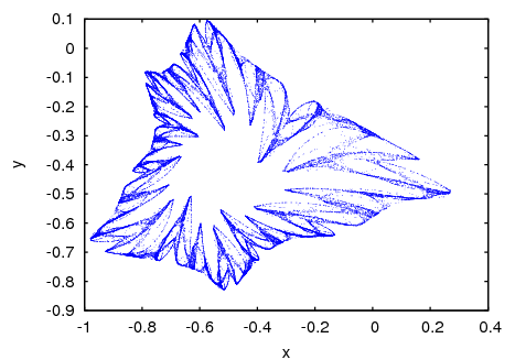
And an enlargement of a small region in that fractal:
(%i9) evolution2d([f,g], [x,y], [-0.5,0], 300000, [x,-0.8,-0.6],
[y,-0.4,-0.2], [style, dots]);
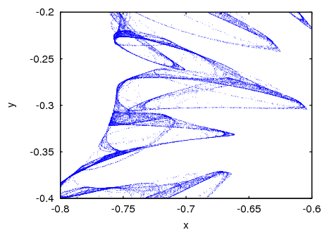
See also: plot2d.
height — Variable
Default value: 500
The height, in pixels, of the graphics window. pixels must be a positive integer number.
ifs (([r1, …, rm], [A1, …, Am], [[x1, y1], …, [xm, ym]], [x0, y0], n, options, …);) — Function
Implements the Iterated Function System method. This method is similar
to the method described in the function chaosgame. but instead of
shrinking the segment from the current point to the randomly chosen
point, the 2 components of that segment will be multiplied by the 2 by 2
matrix Ai that corresponds to the point chosen randomly.
The random choice of one of the m attractive points can be made
with a non-uniform probability distribution defined by the weights
r1,…,rm. Those weights are given in cumulative form; for
instance if there are 3 points with probabilities 0.2, 0.5 and 0.3, the
weights r1, r2 and r3 could be 2, 7 and 10. The
options are the same as for plot2d.
Example. Barnsley’s fern, obtained with 4 matrices and 4 points:
(%i1) a1: matrix([0.85,0.04],[-0.04,0.85])$
(%i2) a2: matrix([0.2,-0.26],[0.23,0.22])$
(%i3) a3: matrix([-0.15,0.28],[0.26,0.24])$
(%i4) a4: matrix([0,0],[0,0.16])$
(%i5) p1: [0,1.6]$
(%i6) p2: [0,1.6]$
(%i7) p3: [0,0.44]$
(%i8) p4: [0,0]$
(%i9) w: [85,92,99,100]$
(%i10) ifs(w, [a1,a2,a3,a4], [p1,p2,p3,p4], [5,0], 50000, [style,dots]);
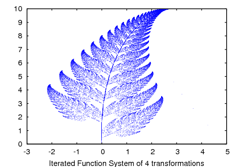
See also: chaosgame, plot2d.
linewidth — Variable
Default value: 1
The width of the lines, when option object_005fwireframe is
used. value must be a positive number.
See also: object_wireframe.
opacity — Variable
Default value: 1
value must be a number between 0 and 1. The lower the number, the more transparent the object will become. The default value of 1 means a completely opaque object.
orbits ((F, y0, n1, n2, [x, x0, xf, xstep], options, …);) — Function
Draws the orbits diagram for a family of one-dimensional discrete dynamical systems, with one parameter x; that kind of diagram is used to study the bifurcations of an one-dimensional discrete system.
The function F(y) defines a sequence with a starting value of
y0, as in the case of the function evolution, but in this
case that function will also depend on a parameter x that will
take values in the interval from x0 to xf with increments of
xstep. Each value used for the parameter x is shown on the
horizontal axis. The vertical axis will show the n2 values
of the sequence y(n1+1),…, y(n1+n2+1) obtained after letting
the sequence evolve n1 iterations. In addition to the options
accepted by plot2d, it accepts an option pixels that
sets up the maximum number of different points that will be represented
in the vertical direction.
Example. Orbits diagram of the quadratic map, with a parameter a:
(%i1) orbits(x^2+a, 0, 50, 200, [a, -2, 0.25], [style, dots]);
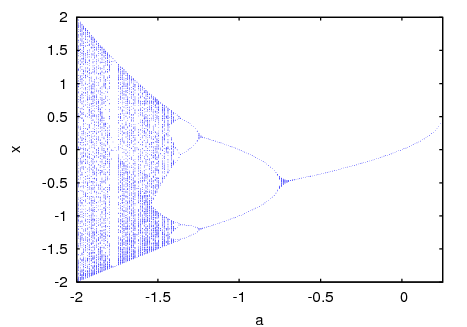
To enlarge the region around the lower bifurcation near x = -1.25 use:
(%i2) orbits(x^2+a, 0, 100, 400, [a,-1,-1.53], [x,-1.6,-0.8],
[nticks, 400], [style,dots]);
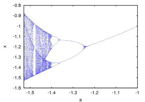
See also: plot2d.
orientation — Variable
Default value: [0, 0, 0]
Three angles by which the object will be rotated with respect to the
three axis. angles can be a list with 3 real numbers, or 3 real
numbers separated by commas. Example: [0, 0, 90] rotates
the x axis of the object to the y axis of the reference frame.
origin — Variable
Default value: [0, 0, 0]
The coordinates of the object’s origin, with respect to which its other dimensions are defined. point can be a list with 3 real numbers, or 3 real numbers separated by commas.
phiresolution — Variable
Default value: ``
The number of sub-intervals into which the phi angle interval from
object_005fstartphi to object_005fendphi
will be divided. num must be a positive integer.
See also object_005fstartphi and
object_005fendphi.
See also: object_startphi, object_endphi.
pointsize — Variable
Default value: 1
The size of the points, when option object_005fpoints is
used. value must be a positive number.
See also: object_points.
position — Variable
Default value: [0, 0, 0]
The coordinates of the object’s position. point can be a list with 3 real numbers, or 3 real numbers separated by commas.
radius — Variable
Default value: 0.5
The radius or a sphere or the distance from the axis to the base’s vertices in a cylinder or a cone. value must be a positive number.
resolution — Variable
Default value: 6
number must be an integer greater than 2 that sets the number of edges in the base of a cone or a cylinder.
restart — Variable
Default value: false
A true value means that animations will restart automatically when the end of the list is reached. Writing just “restart” is equivalent to [restart, true].
scale — Variable
Default value: [1, 1, 1]
Three numbers by which the object will be scaled with respect to the
three axis. factors can be a list with 3 real numbers, or 3 real
numbers separated by commas. Example: [2, 0.5, 1]
enlarges the object to twice its size in the x direction, reduces the
dimensions in the y direction to half and leaves the z dimensions
unchanged.
scene ((objects, …, options, …);) — Function
Accepts an empty list or a list of several scene_005fobjects
and scene_005foptions. The program launches Xmaxima, which
opens an external window representing the given objects in a
3-dimensional space and applying the options given. Each object must
belong to one of the following 4 classes: sphere, cube, cylinder or cone
(see scene_005fobjects). Objects are identified by
giving their name or by a list in which the first element is the class
name and the following elements are options for that object.
Example. A hexagonal pyramid with a blue background:
(%i1) scene(cone, [background,"#9980e5"])$

By holding down the left button of the mouse while it is moved on the
graphics window, the camera can be rotated showing different views of
the pyramid. The two plot options scene_005felevation and
scene_005fazimuth can also be used to change the initial
orientation of the viewing camera. The camera can be moved by holding
the middle mouse button while moving it and holding the right-side mouse
button while moving it up or down will zoom in or out.
Each object option should be a list starting with the option name,
followed by its value. The list of allowed options can be found in the
object_005foptions section.
Example. This will show a sphere falling to the ground and bouncing off without losing any energy. To start or pause the animation, press the play/pause button.
(%i1) p: makelist ([0,0,2.1- 9.8*t^2/2], t, 0, 0.64, 0.01)$
(%i2) p: append (p, reverse(p))$
(%i3) ball: [sphere, [radius,0.1], [thetaresolution,20],
[phiresolution,20], [position,0,0,2.1], [color,red],
[animate,position,p]]$
(%i4) ground: [cube, [xlength,2], [ylength,2], [zlength,0.2],
[position,0,0,-0.1],[color,violet]]$
(%i5) scene (ball, ground, restart)$
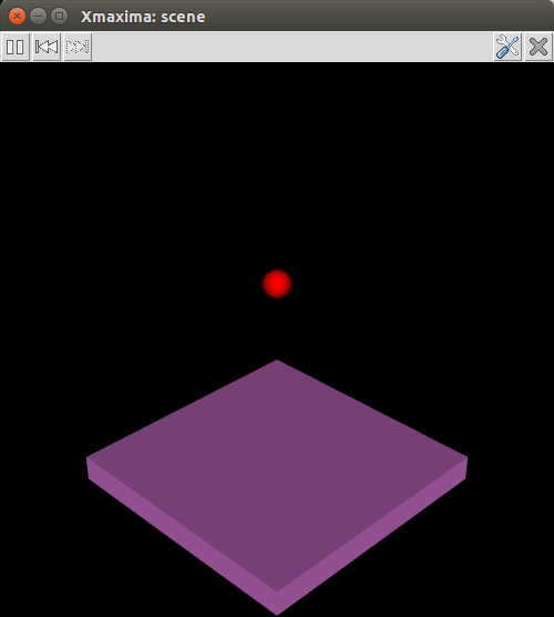
The restart option was used to make the animation restart
automatically every time the last point in the position list is reached.
The accepted values for the colors are the same as for the color
option of plot2d.
See also: scene_objects, scene_options, scene_elevation, scene_azimuth, object_options, color.
sphere — Variable
A sphere with default radius of 0.5 units and center at the origin.
staircase ((F, y0, n, options, …);) — Function
Draws a staircase diagram for the sequence defined by the recurrence relation
y(n+1) = F(y(n))
$$y_{n+1} = F(y_n)$$
The interpretation and allowed values of the input parameters is the
same as for the function evolution. A staircase diagram consists
of a plot of the function F(y), together with the line G(y)
= y. A vertical segment is drawn from the point (y0,
y0) on that line until the point where it intersects the function
F. From that point a horizontal segment is drawn until it reaches
the point (y1, y1) on the line, and the procedure is
repeated n times until the point (yn, yn) is
reached. The options are the same as for plot2d.
Example.
(%i1) staircase(cos(y), 1, 11, [y, 0, 1.2]);
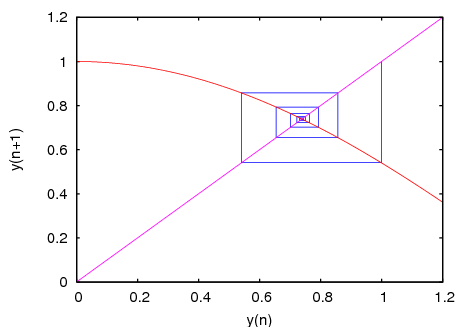
See also: evolution, plot2d.
startphi — Variable
Default value: 0
In a sphere phi is the angle on the vertical plane that passes through the z axis, measured from the positive part of the z axis. angle must be a number between 0 and 180 that sets the initial value of phi at which the surface will start. A value bigger than 0 will eliminate a part of the sphere’s surface.
See also object_005fendphi and
object_005fphiresolution.
See also: object_endphi, object_phiresolution.
starttheta — Variable
Default value: 0
In a sphere theta is the angle on the horizontal plane (longitude), measured from the positive part of the x axis. angle must be a number between 0 and 360 that sets the initial value of theta at which the surface will start. A value bigger than 0 will eliminate a part of the sphere’s surface.
See also object_005fendtheta and
object_005fthetaresolution.
See also: object_endtheta, object_thetaresolution.
surface — Variable
The surfaces of the object will be rendered and the lines and points of
the triangulation used to build the surface will not be shown. This is
the default behavior, which can be changed using either the option
object_005fpoints or object_005fwireframe.
See also: object_points, object_wireframe.
thetaresolution — Variable
Default value: ``
The number of sub-intervals into which the theta angle interval from
object_005fstarttheta to object_005fendtheta
will be divided. num must be a positive integer.
See also object_005fstarttheta and
object_005fendtheta.
See also: object_starttheta, object_endtheta.
track — Variable
positions should be a list of points. When the play button is
pressed, the object position will be changed sequentially through all
the points in the list, at intervals of time given by the option
scene_005ftstep, leaving behind a track of the object’s
trajectory. The rewind button can be used to point at the start of the
sequence making the animation restart after the play button is pressed
again.
Example. This will show the trajectory of a ball thrown with speed of 5 m/s, at an angle of 45 degrees, when the air resistance can be neglected:
(%i1) p: makelist ([0,4*t,4*t- 9.8*t^2/2], t, 0, 0.82, 0.01)$
(%i2) ball: [sphere, [radius,0.1], [color,red], [track,p]]$
(%i3) ground: [cube, [xlength,2], [ylength,4], [zlength,0.2],
[position,0,1.5,-0.2],[color,green]]$
(%i4) scene (ball, ground)$
See also object_005fanimation.
See also: scene_tstep, object_animation.
tstep — Variable
Default value: 10
The amount of time, in mili-seconds, between iterations among consecutive animation frames. time must be a real number.
width — Variable
Default value: 500
The width, in pixels, of the graphics window. pixels must be a positive integer number.
windowname — Variable
Default value: .scene
name must be a string that can be used as the name of the Tk
window created by Xmaxima for the scene graphics. The default
value .scene implies that a new top level window will be created.
windowtitle — Variable
Default value: Xmaxima: scene
name must be a string that will be written in the title of the
window created by scene.
wireframe — Variable
Only the edges of the triangulation used to render the surface will be
shown. Example: [cube, [wireframe]]
See also object_005fsurface and
object_005fpoints.
See also: object_surface, object_points.
xlength — Variable
Default value: 1
The height of a cube in the x direction. length must be a positive
number. See also object_005fylength and
object_005fzlength.
See also: object_ylength, object_zlength.
ylength — Variable
Default value: 1
The height of a cube in the y direction. length must be a positive
number. See also object_005fxlength and
object_005fzlength.
See also: object_xlength, object_zlength.
zlength — Variable
Default value: 1
The height of a cube in z the direction. length must be a positive
number. See also object_005fxlength and
object_005fylength.
See also: object_xlength, object_ylength.
graphs
add_edge (e, gr) — Function
Adds the edge e to the graph gr.
Example:
(%i1) load ("graphs")$
(%i2) p : path_graph(4)$
(%i3) neighbors(0, p);
(%o3) [1]
(%i4) add_edge([0,3], p);
(%o4) done
(%i5) neighbors(0, p);
(%o5) [3, 1]
add_edges (e_list, gr) — Function
Adds all edges in the list e_list to the graph gr.
Example:
(%i1) load ("graphs")$
(%i2) g : empty_graph(3)$
(%i3) add_edges([[0,1],[1,2]], g)$
(%i4) print_graph(g)$
Graph on 3 vertices with 2 edges.
Adjacencies:
2 : 1
1 : 2 0
0 : 1
add_vertex (v, gr) — Function
Adds the vertex v to the graph gr.
Example:
(%i1) load ("graphs")$
(%i2) g : path_graph(2)$
(%i3) add_vertex(2, g)$
(%i4) print_graph(g)$
Graph on 3 vertices with 1 edges.
Adjacencies:
2 :
1 : 0
0 : 1
add_vertices (v_list, gr) — Function
Adds all vertices in the list v_list to the graph gr. A vertex may be any integer, and v_list may contain vertices in any order.
adjacency_matrix (gr) — Function
Returns the adjacency matrix of the graph gr.
Example:
(%i1) load ("graphs")$
(%i2) c5 : cycle_graph(4)$
(%i3) adjacency_matrix(c5);
[ 0 1 0 1 ]
[ ]
[ 1 0 1 0 ]
(%o3) [ ]
[ 0 1 0 1 ]
[ ]
[ 1 0 1 0 ]
average_degree (gr) — Function
Returns the average degree of vertices in the graph gr.
Example:
(%i1) load ("graphs")$
(%i2) average_degree(grotzch_graph());
40
(%o2) --
11
biconnected_components (gr) — Function
Returns the (vertex sets of) 2-connected components of the graph gr.
Example:
(%i1) load ("graphs")$
(%i2) g : create_graph(
[1,2,3,4,5,6,7],
[
[1,2],[2,3],[2,4],[3,4],
[4,5],[5,6],[4,6],[6,7]
])$
(%i3) biconnected_components(g);
(%o3) [[6, 7], [4, 5, 6], [1, 2], [2, 3, 4]]
(Figure graphs13, Graph with 2-connected vertices)
bipartition (gr) — Function
Returns a bipartition of the vertices of the graph gr or an empty list if gr is not bipartite.
Example:
(%i1) load ("graphs")$
(%i2) h : heawood_graph()$
(%i3) [A,B]:bipartition(h);
(%o3) [[8, 12, 6, 10, 0, 2, 4], [13, 5, 11, 7, 9, 1, 3]]
(%i4) draw_graph(h, show_vertices=A, program=circular)$
(Figure graphs02, Bipartition of the vertices in a Heawood graph)
chromatic_index (gr) — Function
Returns the chromatic index of the graph gr.
Example:
(%i1) load ("graphs")$
(%i2) p : petersen_graph()$
(%i3) chromatic_index(p);
(%o3) 4
chromatic_number (gr) — Function
Returns the chromatic number of the graph gr.
Example:
(%i1) load ("graphs")$
(%i2) chromatic_number(cycle_graph(5));
(%o2) 3
(%i3) chromatic_number(cycle_graph(6));
(%o3) 2
circulant_graph (n, d) — Function
Returns the circulant graph with parameters n and d.
Example:
(%i1) load ("graphs")$
(%i2) g : circulant_graph(10, [1,3])$
(%i3) print_graph(g)$
Graph on 10 vertices with 20 edges.
Adjacencies:
9 : 2 6 0 8
8 : 1 5 9 7
7 : 0 4 8 6
6 : 9 3 7 5
5 : 8 2 6 4
4 : 7 1 5 3
3 : 6 0 4 2
2 : 9 5 3 1
1 : 8 4 2 0
0 : 7 3 9 1
clear_edge_weight (e, gr) — Function
Removes the weight of the edge e in the graph gr.
Example:
(%i1) load ("graphs")$
(%i2) g : create_graph(3, [[[0,1], 1.5], [[1,2], 1.3]])$
(%i3) get_edge_weight([0,1], g);
(%o3) 1.5
(%i4) clear_edge_weight([0,1], g)$
(%i5) get_edge_weight([0,1], g);
(%o5) 1
clear_vertex_label (v, gr) — Function
Removes the label of the vertex v in the graph gr.
Example:
(%i1) load ("graphs")$
(%i2) g : create_graph([[0,"Zero"], [1, "One"]], [[0,1]])$
(%i3) get_vertex_label(0, g);
(%o3) Zero
(%i4) clear_vertex_label(0, g);
(%o4) done
(%i5) get_vertex_label(0, g);
(%o5) false
clebsch_graph () — Function
Returns the Clebsch graph.
complement_graph (g) — Function
Returns the complement of the graph g.
complete_bipartite_graph (n, m) — Function
Returns the complete bipartite graph on n+m vertices.
complete_graph (n) — Function
Returns the complete graph on n vertices.
connect_vertices (v_list, u_list, gr) — Function
Connects all vertices from the list v_list with the vertices in the list u_list in the graph gr.
v_list and u_list can be single vertices or lists of vertices.
Example:
(%i1) load ("graphs")$
(%i2) g : empty_graph(4)$
(%i3) connect_vertices(0, [1,2,3], g)$
(%i4) print_graph(g)$
Graph on 4 vertices with 3 edges.
Adjacencies:
3 : 0
2 : 0
1 : 0
0 : 3 2 1
connected_components (gr) — Function
Returns the (vertex sets of) connected components of the graph gr.
Example:
(%i1) load ("graphs")$
(%i2) g: graph_union(cycle_graph(5), path_graph(4))$
(%i3) connected_components(g);
(%o3) [[1, 2, 3, 4, 0], [8, 7, 6, 5]]
contract_edge (e, gr) — Function
Contracts the edge e in the graph gr.
Example:
(%i1) load ("graphs")$
(%i2) g: create_graph(
8, [[0,3],[1,3],[2,3],[3,4],[4,5],[4,6],[4,7]])$
(%i3) print_graph(g)$
Graph on 8 vertices with 7 edges.
Adjacencies:
7 : 4
6 : 4
5 : 4
4 : 7 6 5 3
3 : 4 2 1 0
2 : 3
1 : 3
0 : 3
(%i4) contract_edge([3,4], g)$
(%i5) print_graph(g)$
Graph on 7 vertices with 6 edges.
Adjacencies:
7 : 3
6 : 3
5 : 3
3 : 5 6 7 2 1 0
2 : 3
1 : 3
0 : 3
copy_graph (g) — Function
Returns a copy of the graph g.
create_graph (v_list, e_list) — Function
Creates a new graph on the set of vertices v_list and with edges e_list.
v_list is a list of vertices [v1, v2, ..., vn] or a
list of vertices together with vertex labels [[v1, l1], [v2 ,l2], ..., [vn, ln]].
A vertex may be any integer,
and v_list may contain vertices in any order.
A label may be any Maxima expression,
and two or more vertices may have the same label.
n is the number of vertices. Vertices will be identified by integers from 0 to n-1.
e_list is a list of edges [e1, e2,..., em] or a list of
edges together with edge-weights [[e1, w1], ..., [em, wm]].
If directed is not false, a directed graph will be returned.
Example 1: create a cycle on 3 vertices:
(%i1) load ("graphs")$
(%i2) g : create_graph([1,2,3], [[1,2], [2,3], [1,3]])$
(%i3) print_graph(g)$
Graph on 3 vertices with 3 edges.
Adjacencies:
3 : 1 2
2 : 3 1
1 : 3 2
Example 2: create a cycle on 3 vertices with edge weights:
(%i1) load ("graphs")$
(%i2) g : create_graph([1,2,3], [[[1,2], 1.0], [[2,3], 2.0],
[[1,3], 3.0]])$
(%i3) print_graph(g)$
Graph on 3 vertices with 3 edges.
Adjacencies:
3 : 1 2
2 : 3 1
1 : 3 2
Example 3: create a directed graph:
(%i1) load ("graphs")$
(%i2) d : create_graph(
[1,2,3,4],
[
[1,3], [1,4],
[2,3], [2,4]
],
'directed = true)$
(%i3) print_graph(d)$
Digraph on 4 vertices with 4 arcs.
Adjacencies:
4 :
3 :
2 : 4 3
1 : 4 3
cube_graph (n) — Function
Returns the n-dimensional cube.
cuboctahedron_graph (n) — Function
Returns the cuboctahedron graph.
cycle_digraph (n) — Function
Returns the directed cycle on n vertices.
cycle_graph (n) — Function
Returns the cycle on n vertices.
degree_sequence (gr) — Function
Returns the list of vertex degrees of the graph gr.
Example:
(%i1) load ("graphs")$
(%i2) degree_sequence(random_graph(10, 0.4));
(%o2) [2, 2, 2, 2, 2, 2, 3, 3, 3, 3]
diameter (gr) — Function
Returns the diameter of the graph gr.
Example:
(%i1) load ("graphs")$
(%i2) diameter(dodecahedron_graph());
(%o2) 5
dimacs_export (gr, fl) — Function
Exports the graph into the file fl in the DIMACS format. Optional comments will be added to the top of the file.
dimacs_import (fl) — Function
Returns the graph from file fl in the DIMACS format.
dodecahedron_graph () — Function
Returns the dodecahedron graph.
draw_graph (graph) — Function
Draws the graph using the Package-draw package.
The algorithm used to position vertices is specified by the optional
argument program. The default value is
program=spring_embedding. draw_graph can also use the
graphviz programs for positioning vertices, but graphviz must be
installed separately.
Example 1:
(%i1) load ("graphs")$
(%i2) g:grid_graph(10,10)$
(%i3) m:max_matching(g)$
(%i4) draw_graph(g,
spring_embedding_depth=100,
show_edges=m, edge_type=dots,
vertex_size=0)$
(Figure graphs09, Example of the use of draw_graph to draw a graph)
Example 2:
(%i1) load ("graphs")$
(%i2) g:create_graph(16,
[
[0,1],[1,3],[2,3],[0,2],[3,4],[2,4],
[5,6],[6,4],[4,7],[6,7],[7,8],[7,10],[7,11],
[8,10],[11,10],[8,9],[11,12],[9,15],[12,13],
[10,14],[15,14],[13,14]
])$
(%i3) t:minimum_spanning_tree(g)$
(%i4) draw_graph(
g,
show_edges=edges(t),
show_edge_width=4,
show_edge_color=green,
vertex_type=filled_square,
vertex_size=2
)$
(Figure graphs10, Example of the use of draw_graph to draw a graph)
Example 3:
(%i1) load ("graphs")$
(%i2) g:create_graph(16,
[
[0,1],[1,3],[2,3],[0,2],[3,4],[2,4],
[5,6],[6,4],[4,7],[6,7],[7,8],[7,10],[7,11],
[8,10],[11,10],[8,9],[11,12],[9,15],[12,13],
[10,14],[15,14],[13,14]
])$
(%i3) mi : max_independent_set(g)$
(%i4) draw_graph(
g,
show_vertices=mi,
show_vertex_type=filled_up_triangle,
show_vertex_size=2,
edge_color=cyan,
edge_width=3,
show_id=true,
text_color=brown
)$
(Figure graphs11, Example of the use of draw_graph to draw a graph)
Example 4:
(%i1) load ("graphs")$
(%i2) net : create_graph(
[0,1,2,3,4,5],
[
[[0,1], 3], [[0,2], 2],
[[1,3], 1], [[1,4], 3],
[[2,3], 2], [[2,4], 2],
[[4,5], 2], [[3,5], 2]
],
directed=true
)$
(%i3) draw_graph(
net,
show_weight=true,
vertex_size=0,
show_vertices=[0,5],
show_vertex_type=filled_square,
head_length=0.2,
head_angle=10,
edge_color="dark-green",
text_color=blue
)$
(Figure graphs12, Example of the use of draw_graph to draw a graph)
Example 5:
(%i1) load("graphs")$
(%i2) g: petersen_graph(20, 2);
(%o2) GRAPH
(%i3) draw_graph(g, redraw=true, program=planar_embedding);
(%o3) done
(Figure graphs14, Example of the use of draw_graph to draw a graph)
Example 6:
(%i1) load("graphs")$
(%i2) t: tutte_graph();
(%o2) GRAPH
(%i3) draw_graph(t, redraw=true,
fixed_vertices=[1,2,3,4,5,6,7,8,9]);
(%o3) done
(Figure graphs15, Example of the use of draw_graph to draw a graph)
See also: Package-draw.
draw_graph_program — Variable
Default value: spring_embedding
The default value for the program used to position vertices in
draw_graph program.
edge_color — Variable
The color used for displaying edges.
edge_coloring (gr) — Function
Returns an optimal coloring of the edges of the graph gr.
The function returns the chromatic index and a list representing the coloring of the edges of gr.
Example:
(%i1) load ("graphs")$
(%i2) p : petersen_graph()$
(%i3) [ch_index, col] : edge_coloring(p);
(%o3) [4, [[[0, 5], 3], [[5, 7], 1], [[0, 1], 1], [[1, 6], 2],
[[6, 8], 1], [[1, 2], 3], [[2, 7], 4], [[7, 9], 2], [[2, 3], 2],
[[3, 8], 3], [[5, 8], 2], [[3, 4], 1], [[4, 9], 4], [[6, 9], 3],
[[0, 4], 2]]]
(%i4) assoc([0,1], col);
(%o4) 1
(%i5) assoc([0,5], col);
(%o5) 3
edge_connectivity (gr) — Function
Returns the edge-connectivity of the graph gr.
See also min_edge_cut.
See also: min_edge_cut.
edge_partition — Variable
A partition [[e1,e2,...],...,[ek,...,em]] of edges of the
graph. The edges of each list in the partition will be drawn using a
different color.
edge_type — Variable
Defines how edges are displayed. See the line_type option for the
draw package.
edge_width — Variable
The width of edges.
edges (gr) — Function
Returns the list of edges (arcs) in a (directed) graph gr.
Example:
(%i1) load ("graphs")$
(%i2) edges(complete_graph(4));
(%o2) [[2, 3], [1, 3], [1, 2], [0, 3], [0, 2], [0, 1]]
empty_graph (n) — Function
Returns the empty graph on n vertices.
fixed_vertices — Variable
Specifies a list of vertices which will have positions fixed along a regular polygon.
Can be used when program=spring_embedding.
flower_snark (n) — Function
Returns the flower graph on 4n vertices.
Example:
(%i1) load ("graphs")$
(%i2) f5 : flower_snark(5)$
(%i3) chromatic_index(f5);
(%o3) 4
from_adjacency_matrix (A) — Function
Returns the graph represented by its adjacency matrix A.
frucht_graph () — Function
Returns the Frucht graph.
get_all_vertices_by_label (l, gr) — Function
Returns all vertices, if any, which have the label l in graph gr.
If there are no such vertices,
get_all_vertices_by_label returns an empty list [].
Example:
(%i1) load ("graphs")$
(%i2) g: create_graph ([[0, "Zero"], [1, "One"], [2, "Other"], [3, "Other"]], []) $
(%i3) get_all_vertices_by_label ("Zero", g);
(%o3) [0]
(%i4) get_all_vertices_by_label ("Two", g);
(%o4) []
(%i5) get_all_vertices_by_label ("Other", g);
(%o5) [2, 3]
get_edge_weight (e, gr) — Function
Returns the weight of the edge e in the graph gr.
If there is no weight assigned to the edge, the function returns 1. If the edge is not present in the graph, the function signals an error or returns the optional argument ifnot.
Example:
(%i1) load ("graphs")$
(%i2) c5 : cycle_graph(5)$
(%i3) get_edge_weight([1,2], c5);
(%o3) 1
(%i4) set_edge_weight([1,2], 2.0, c5);
(%o4) done
(%i5) get_edge_weight([1,2], c5);
(%o5) 2.0
get_unique_vertex_by_label (l, gr) — Function
Returns the unique vertex which has the label l in graph gr.
If there is no such vertex,
get_unique_vertex_by_label returns false.
If there are two or more vertices with label l,
get_unique_vertex_by_label reports an error.
Example:
(%i1) load ("graphs")$
(%i2) g: create_graph ([[0, "Zero"], [1, "One"], [2, "Other"], [3, "Other"]], []) $
(%i3) get_unique_vertex_by_label ("Zero", g);
(%o3) 0
(%i4) get_unique_vertex_by_label ("Two", g);
(%o4) false
(%i5) errcatch (get_unique_vertex_by_label ("Other", g));
get_unique_vertex_by_label: two or more vertices have the same label "Other"
(%o5) []
get_vertex_label (v, gr) — Function
Returns the label of the vertex v in the graph gr.
If no label is assigned to vertex v,
get_vertex_label returns false.
Example:
(%i1) load("graphs")$
(%i2) g: create_graph([[0, "Zero"], [1, "One"], 2, 3], [])$
(%i3) get_vertex_label(0, g);
(%o3) Zero
(%i4) get_vertex_label(2, g);
(%o4) false
girth (gr) — Function
Returns the length of the shortest cycle in gr.
Example:
(%i1) load ("graphs")$
(%i2) g : heawood_graph()$
(%i3) girth(g);
(%o3) 6
graph6_decode (str) — Function
Returns the graph encoded in the graph6 format in the string str.
graph6_encode (gr) — Function
Returns a string which encodes the graph gr in the graph6 format.
graph6_export (gr_list, fl) — Function
Exports graphs in the list gr_list to the file fl in the graph6 format.
graph6_import (fl) — Function
Returns a list of graphs from the file fl in the graph6 format.
graph_center (gr) — Function
Returns the center of the graph gr.
Example:
(%i1) load ("graphs")$
(%i2) g : grid_graph(5,5)$
(%i3) graph_center(g);
(%o3) [12]
graph_charpoly (gr, x) — Function
Returns the characteristic polynomial (in variable x) of the graph gr.
Example:
(%i1) load ("graphs")$
(%i2) p : petersen_graph()$
(%i3) graph_charpoly(p, x), factor;
5 4
(%o3) (x - 3) (x - 1) (x + 2)
graph_eigenvalues (gr) — Function
Returns the eigenvalues of the graph gr. The function returns
eigenvalues in the same format as maxima eigenvalues function.
Example:
(%i1) load ("graphs")$
(%i2) p : petersen_graph()$
(%i3) graph_eigenvalues(p);
(%o3) [[3, - 2, 1], [1, 4, 5]]
See also: eigenvalues.
graph_order (gr) — Function
Returns the number of vertices in the graph gr.
Example:
(%i1) load ("graphs")$
(%i2) p : petersen_graph()$
(%i3) graph_order(p);
(%o3) 10
graph_periphery (gr) — Function
Returns the periphery of the graph gr.
Example:
(%i1) load ("graphs")$
(%i2) g : grid_graph(5,5)$
(%i3) graph_periphery(g);
(%o3) [24, 20, 4, 0]
graph_product (g1, g1) — Function
Returns the direct product of graphs g1 and g2.
Example:
(%i1) load ("graphs")$
(%i2) grid : graph_product(path_graph(3), path_graph(4))$
(%i3) draw_graph(grid)$
(Figure graphs01, Direct product of two graphs)
graph_size (gr) — Function
Returns the number of edges in the graph gr.
Example:
(%i1) load ("graphs")$
(%i2) p : petersen_graph()$
(%i3) graph_size(p);
(%o3) 15
graph_union (g1, g1) — Function
Returns the union (sum) of graphs g1 and g2.
great_rhombicosidodecahedron_graph () — Function
Returns the great rhombicosidodecahedron graph.
great_rhombicuboctahedron_graph () — Function
Returns the great rhombicuboctahedron graph.
grid_graph (n, m) — Function
Returns the n x m grid.
grotzch_graph () — Function
Returns the Grotzch graph.
hamilton_cycle (gr) — Function
Returns the Hamilton cycle of the graph gr or an empty list if gr is not hamiltonian.
Example:
(%i1) load ("graphs")$
(%i2) c : cube_graph(3)$
(%i3) hc : hamilton_cycle(c);
(%o3) [7, 3, 2, 6, 4, 0, 1, 5, 7]
(%i4) draw_graph(c, show_edges=vertices_to_cycle(hc))$
(Figure graphs03, Hamilton cycle of a cubic graph)
hamilton_path (gr) — Function
Returns the Hamilton path of the graph gr or an empty list if gr does not have a Hamilton path.
Example:
(%i1) load ("graphs")$
(%i2) p : petersen_graph()$
(%i3) hp : hamilton_path(p);
(%o3) [0, 5, 7, 2, 1, 6, 8, 3, 4, 9]
(%i4) draw_graph(p, show_edges=vertices_to_path(hp))$
(Figure graphs04, Hamilton path of a Petersen graph)
heawood_graph () — Function
Returns the Heawood graph.
icosahedron_graph () — Function
Returns the icosahedron graph.
icosidodecahedron_graph () — Function
Returns the icosidodecahedron graph.
in_neighbors (v, gr) — Function
Returns the list of in-neighbors of the vertex v in the directed graph gr.
Example:
(%i1) load ("graphs")$
(%i2) p : path_digraph(3)$
(%i3) in_neighbors(2, p);
(%o3) [1]
(%i4) out_neighbors(2, p);
(%o4) []
induced_subgraph (V, g) — Function
Returns the graph induced on the subset V of vertices of the graph g.
Example:
(%i1) load ("graphs")$
(%i2) p : petersen_graph()$
(%i3) V : [0,1,2,3,4]$
(%i4) g : induced_subgraph(V, p)$
(%i5) print_graph(g)$
Graph on 5 vertices with 5 edges.
Adjacencies:
4 : 3 0
3 : 2 4
2 : 1 3
1 : 0 2
0 : 1 4
is_biconnected (gr) — Function
Returns true if gr is 2-connected and false otherwise.
Example:
(%i1) load ("graphs")$
(%i2) is_biconnected(cycle_graph(5));
(%o2) true
(%i3) is_biconnected(path_graph(5));
(%o3) false
is_bipartite (gr) — Function
Returns true if gr is bipartite (2-colorable) and false otherwise.
Example:
(%i1) load ("graphs")$
(%i2) is_bipartite(petersen_graph());
(%o2) false
(%i3) is_bipartite(heawood_graph());
(%o3) true
is_connected (gr) — Function
Returns true if the graph gr is connected and false otherwise.
Example:
(%i1) load ("graphs")$
(%i2) is_connected(graph_union(cycle_graph(4), path_graph(3)));
(%o2) false
is_digraph (gr) — Function
Returns true if gr is a directed graph and false otherwise.
Example:
(%i1) load ("graphs")$
(%i2) is_digraph(path_graph(5));
(%o2) false
(%i3) is_digraph(path_digraph(5));
(%o3) true
is_edge_in_graph (e, gr) — Function
Returns true if e is an edge (arc) in the (directed) graph g
and false otherwise.
Example:
(%i1) load ("graphs")$
(%i2) c4 : cycle_graph(4)$
(%i3) is_edge_in_graph([2,3], c4);
(%o3) true
(%i4) is_edge_in_graph([3,2], c4);
(%o4) true
(%i5) is_edge_in_graph([2,4], c4);
(%o5) false
(%i6) is_edge_in_graph([3,2], cycle_digraph(4));
(%o6) false
is_graph (gr) — Function
Returns true if gr is a graph and false otherwise.
Example:
(%i1) load ("graphs")$
(%i2) is_graph(path_graph(5));
(%o2) true
(%i3) is_graph(path_digraph(5));
(%o3) false
is_graph_or_digraph (gr) — Function
Returns true if gr is a graph or a directed graph and false otherwise.
Example:
(%i1) load ("graphs")$
(%i2) is_graph_or_digraph(path_graph(5));
(%o2) true
(%i3) is_graph_or_digraph(path_digraph(5));
(%o3) true
is_isomorphic (gr1, gr2) — Function
Returns true if graphs/digraphs gr1 and gr2 are isomorphic
and false otherwise.
See also isomorphism.
Example:
(%i1) load ("graphs")$
(%i2) clk5:complement_graph(line_graph(complete_graph(5)))$
(%i3) is_isomorphic(clk5, petersen_graph());
(%o3) true
See also: isomorphism.
is_planar (gr) — Function
Returns true if gr is a planar graph and false otherwise.
The algorithm used is the Demoucron’s algorithm, which is a quadratic time algorithm.
Example:
(%i1) load ("graphs")$
(%i2) is_planar(dodecahedron_graph());
(%o2) true
(%i3) is_planar(petersen_graph());
(%o3) false
(%i4) is_planar(petersen_graph(10,2));
(%o4) true
is_sconnected (gr) — Function
Returns true if the directed graph gr is strongly connected and
false otherwise.
Example:
(%i1) load ("graphs")$
(%i2) is_sconnected(cycle_digraph(5));
(%o2) true
(%i3) is_sconnected(path_digraph(5));
(%o3) false
is_tree (gr) — Function
Returns true if gr is a tree and false otherwise.
Example:
(%i1) load ("graphs")$
(%i2) is_tree(random_tree(4));
(%o2) true
(%i3) is_tree(graph_union(random_tree(4), random_tree(5)));
(%o3) false
is_vertex_in_graph (v, gr) — Function
Returns true if v is a vertex in the graph g and false otherwise.
Example:
(%i1) load ("graphs")$
(%i2) c4 : cycle_graph(4)$
(%i3) is_vertex_in_graph(0, c4);
(%o3) true
(%i4) is_vertex_in_graph(6, c4);
(%o4) false
isomorphism (gr1, gr2) — Function
Returns a an isomorphism between graphs/digraphs gr1 and gr2. If gr1 and gr2 are not isomorphic, it returns an empty list.
Example:
(%i1) load ("graphs")$
(%i2) clk5:complement_graph(line_graph(complete_graph(5)))$
(%i3) isomorphism(clk5, petersen_graph());
(%o3) [9 -> 0, 2 -> 1, 6 -> 2, 5 -> 3, 0 -> 4, 1 -> 5, 3 -> 6,
4 -> 7, 7 -> 8, 8 -> 9]
laplacian_matrix (gr) — Function
Returns the laplacian matrix of the graph gr.
Example:
(%i1) load ("graphs")$
(%i2) laplacian_matrix(cycle_graph(5));
[ 2 - 1 0 0 - 1 ]
[ ]
[ - 1 2 - 1 0 0 ]
[ ]
(%o2) [ 0 - 1 2 - 1 0 ]
[ ]
[ 0 0 - 1 2 - 1 ]
[ ]
[ - 1 0 0 - 1 2 ]
line_graph (g) — Function
Returns the line graph of the graph g.
make_graph (vrt, f) — Function
Creates a graph using a predicate function f.
vrt is a list or set of vertices, or an integer.
When vrt is a list or set, its elements may be any integers, and, if a list, may be listed in any order.
When vrt is an integer, vertices of the graph will be integers from 1 to vrt.
f is a predicate function. Two vertices a and b will
be connected if f(a,b)=true.
If directed is not false, then the graph will be directed.
Example 1:
(%i1) load("graphs")$
(%i2) g : make_graph(powerset({1,2,3,4,5}, 2), disjointp)$
(%i3) is_isomorphic(g, petersen_graph());
(%o3) true
(%i4) get_vertex_label(1, g);
(%o4) {1, 2}
Example 2:
(%i1) load("graphs")$
(%i2) f(i, j) := is (mod(j, i)=0)$
(%i3) g : make_graph(20, f, directed=true)$
(%i4) out_neighbors(4, g);
(%o4) [8, 12, 16, 20]
(%i5) in_neighbors(18, g);
(%o5) [1, 2, 3, 6, 9]
max_clique (gr) — Function
Returns a maximum clique of the graph gr.
Example:
(%i1) load ("graphs")$
(%i2) g : random_graph(100, 0.5)$
(%i3) max_clique(g);
(%o3) [6, 12, 31, 36, 52, 59, 62, 63, 80]
max_degree (gr) — Function
Returns the maximal degree of vertices of the graph gr and a vertex of maximal degree.
Example:
(%i1) load ("graphs")$
(%i2) g : random_graph(100, 0.02)$
(%i3) max_degree(g);
(%o3) [6, 79]
(%i4) vertex_degree(95, g);
(%o4) 2
max_flow (net, s, t) — Function
Returns a maximum flow through the network net with the source s and the sink t.
The function returns the value of the maximal flow and a list representing the weights of the arcs in the optimal flow.
Example:
(%i1) load ("graphs")$
(%i2) net : create_graph(
[1,2,3,4,5,6],
[[[1,2], 1.0],
[[1,3], 0.3],
[[2,4], 0.2],
[[2,5], 0.3],
[[3,4], 0.1],
[[3,5], 0.1],
[[4,6], 1.0],
[[5,6], 1.0]],
directed=true)$
(%i3) [flow_value, flow] : max_flow(net, 1, 6);
(%o3) [0.7, [[[1, 2], 0.5], [[1, 3], 0.2], [[2, 4], 0.2],
[[2, 5], 0.3], [[3, 4], 0.1], [[3, 5], 0.1], [[4, 6], 0.3],
[[5, 6], 0.4]]]
(%i4) fl : 0$
(%i5) for u in out_neighbors(1, net)
do fl : fl + assoc([1, u], flow)$
(%i6) fl;
(%o6) 0.7
max_independent_set (gr) — Function
Returns a maximum independent set of the graph gr.
Example:
(%i1) load ("graphs")$
(%i2) d : dodecahedron_graph()$
(%i3) mi : max_independent_set(d);
(%o3) [0, 3, 5, 9, 10, 11, 18, 19]
(%i4) draw_graph(d, show_vertices=mi)$
(Figure graphs05, Maximum independent set of a dodecahedral graph)
max_matching (gr) — Function
Returns a maximum matching of the graph gr.
Example:
(%i1) load ("graphs")$
(%i2) d : dodecahedron_graph()$
(%i3) m : max_matching(d);
(%o3) [[5, 7], [8, 9], [6, 10], [14, 19], [13, 18], [12, 17],
[11, 16], [0, 15], [3, 4], [1, 2]]
(%i4) draw_graph(d, show_edges=m)$
(Figure graphs06, Maximum matching of a dodecahedral graph)
min_degree (gr) — Function
Returns the minimum degree of vertices of the graph gr and a vertex of minimum degree.
Example:
(%i1) load ("graphs")$
(%i2) g : random_graph(100, 0.1)$
(%i3) min_degree(g);
(%o3) [3, 49]
(%i4) vertex_degree(21, g);
(%o4) 9
min_edge_cut (gr) — Function
Returns the minimum edge cut in the graph gr.
See also edge_005fconnectivity.
See also: edge_connectivity.
min_vertex_cover (gr) — Function
Returns the minimum vertex cover of the graph gr.
min_vertex_cut (gr) — Function
Returns the minimum vertex cut in the graph gr.
See also vertex_005fconnectivity.
See also: vertex_connectivity.
minimum_spanning_tree (gr) — Function
Returns the minimum spanning tree of the graph gr.
Example:
(%i1) load ("graphs")$
(%i2) g : graph_product(path_graph(10), path_graph(10))$
(%i3) t : minimum_spanning_tree(g)$
(%i4) draw_graph(g, show_edges=edges(t))$
(Figure graphs07, Minimum spanning of rectangular graph)
mycielski_graph (g) — Function
Returns the mycielskian graph of the graph g.
neighbors (v, gr) — Function
Returns the list of neighbors of the vertex v in the graph gr.
Example:
(%i1) load ("graphs")$
(%i2) p : petersen_graph()$
(%i3) neighbors(3, p);
(%o3) [4, 8, 2]
new_graph () — Function
Returns the graph with no vertices and no edges.
odd_girth (gr) — Function
Returns the length of the shortest odd cycle in the graph gr.
Example:
(%i1) load ("graphs")$
(%i2) g : graph_product(cycle_graph(4), cycle_graph(7))$
(%i3) girth(g);
(%o3) 4
(%i4) odd_girth(g);
(%o4) 7
out_neighbors (v, gr) — Function
Returns the list of out-neighbors of the vertex v in the directed graph gr.
Example:
(%i1) load ("graphs")$
(%i2) p : path_digraph(3)$
(%i3) in_neighbors(2, p);
(%o3) [1]
(%i4) out_neighbors(2, p);
(%o4) []
path_digraph (n) — Function
Returns the directed path on n vertices.
path_graph (n) — Function
Returns the path on n vertices.
petersen_graph () — Function
Returns the petersen graph P_{n,d}. The default values for
n and d are n=5 and d=2.
planar_embedding (gr) — Function
Returns the list of facial walks in a planar embedding of gr and
false if gr is not a planar graph.
The graph gr must be biconnected.
The algorithm used is the Demoucron’s algorithm, which is a quadratic time algorithm.
Example:
(%i1) load ("graphs")$
(%i2) planar_embedding(grid_graph(3,3));
(%o2) [[3, 6, 7, 8, 5, 2, 1, 0], [4, 3, 0, 1], [3, 4, 7, 6],
[8, 7, 4, 5], [1, 2, 5, 4]]
print_graph (gr) — Function
Prints some information about the graph gr.
Example:
(%i1) load ("graphs")$
(%i2) c5 : cycle_graph(5)$
(%i3) print_graph(c5)$
Graph on 5 vertices with 5 edges.
Adjacencies:
4 : 0 3
3 : 4 2
2 : 3 1
1 : 2 0
0 : 4 1
(%i4) dc5 : cycle_digraph(5)$
(%i5) print_graph(dc5)$
Digraph on 5 vertices with 5 arcs.
Adjacencies:
4 : 0
3 : 4
2 : 3
1 : 2
0 : 1
(%i6) out_neighbors(0, dc5);
(%o6) [1]
program — Variable
Defines the program used for positioning vertices of the graph. Can be
one of the graphviz programs (dot, neato, twopi, circ, fdp),
circular, spring_embedding or
planar_embedding. planar_embedding is only available for
2-connected planar graphs. When program=spring_embedding, a set
of vertices with fixed position can be specified with the
fixed_vertices option.
random_bipartite_graph (a, b, p) — Function
Returns a random bipartite graph on a+b vertices. Each edge is
present with probability p.
random_digraph (n, p) — Function
Returns a random directed graph on n vertices. Each arc is present with probability p.
random_graph (n, p) — Function
Returns a random graph on n vertices. Each edge is present with probability p.
random_graph1 (n, m) — Function
Returns a random graph on n vertices and random m edges.
random_network (n, p, w) — Function
Returns a random network on n vertices. Each arc is present with
probability p and has a weight in the range [0,w]. The
function returns a list [network, source, sink].
Example:
(%i1) load ("graphs")$
(%i2) [net, s, t] : random_network(50, 0.2, 10.0);
(%o2) [DIGRAPH, 50, 51]
(%i3) max_flow(net, s, t)$
(%i4) first(%);
(%o4) 27.65981397932507
random_regular_graph (n) — Function
Returns a random d-regular graph on n vertices. The default
value for d is d=3.
random_tournament (n) — Function
Returns a random tournament on n vertices.
random_tree (n) — Function
Returns a random tree on n vertices.
redraw — Variable
Default value: false
If true, vertex positions are recomputed even if the positions
have been saved from a previous drawing of the graph.
remove_edge (e, gr) — Function
Removes the edge e from the graph gr.
Example:
(%i1) load ("graphs")$
(%i2) c3 : cycle_graph(3)$
(%i3) remove_edge([0,1], c3)$
(%i4) print_graph(c3)$
Graph on 3 vertices with 2 edges.
Adjacencies:
2 : 0 1
1 : 2
0 : 2
remove_vertex (v, gr) — Function
Removes the vertex v from the graph gr.
set_edge_weight (e, w, gr) — Function
Assigns the weight w to the edge e in the graph gr.
Example:
(%i1) load ("graphs")$
(%i2) g : create_graph([1, 2], [[[1,2], 1.2]])$
(%i3) get_edge_weight([1,2], g);
(%o3) 1.2
(%i4) set_edge_weight([1,2], 2.1, g);
(%o4) done
(%i5) get_edge_weight([1,2], g);
(%o5) 2.1
set_vertex_label (v, l, gr) — Function
Assigns the label l to the vertex v in the graph gr.
A label may be any Maxima expression, and two or more vertices may have the same label.
Example:
(%i1) load ("graphs")$
(%i2) g : create_graph([[1, "One"], [2, "Two"]], [[1, 2]])$
(%i3) get_vertex_label(1, g);
(%o3) One
(%i4) set_vertex_label(1, "oNE", g);
(%o4) done
(%i5) get_vertex_label(1, g);
(%o5) oNE
(%i6) h : create_graph([[11, x], [22, y], [33, x + y]], [[11, 33], [22, 33]]) $
(%i7) get_vertex_label (33, h);
(%o7) y + x
shortest_path (u, v, gr) — Function
Returns the shortest path from u to v in the graph gr.
Example:
(%i1) load ("graphs")$
(%i2) d : dodecahedron_graph()$
(%i3) path : shortest_path(0, 7, d);
(%o3) [0, 1, 19, 13, 7]
(%i4) draw_graph(d, show_edges=vertices_to_path(path))$
(Figure graphs08, Shortest path between two vertices in a dodecahedral graph)
shortest_weighted_path (u, v, gr) — Function
Returns the length of the shortest weighted path and the shortest weighted path from u to v in the graph gr.
The length of a weighted path is the sum of edge weights of edges in the path. If an edge has no weight, then it has a default weight 1.
Example:
(%i1) load ("graphs")$
(%i2) g: petersen_graph(20, 2)$
(%i3) for e in edges(g) do set_edge_weight(e, random(1.0), g)$
(%i4) shortest_weighted_path(0, 10, g);
(%o4) [2.575143920268482, [0, 20, 38, 36, 34, 32, 30, 10]]
show_edge_color — Variable
The color used for displaying edges in the show_edges list.
show_edge_type — Variable
Defines how edges in show_edges are displayed. See the
line_type option for the draw package.
show_edge_width — Variable
The width of edges in show_edges.
show_edges — Variable
Display edges specified in the list e_list using a different color.
show_id — Variable
Default value: false
If true then ids of the vertices are displayed.
show_label — Variable
Default value: false
If true then labels of the vertices are displayed.
show_vertex_color — Variable
The color used for displaying vertices in the show_vertices list.
show_vertex_size — Variable
The size of vertices in show_vertices.
show_vertex_type — Variable
Defines how vertices specified in show_vertices are displayed.
See the point_type option for the draw package for possible
values.
show_vertices — Variable
Default value: []
Display selected vertices in the using a different color.
show_weight — Variable
Default value: false
If true then weights of the edges are displayed.
small_rhombicosidodecahedron_graph () — Function
Returns the small rhombicosidodecahedron graph.
small_rhombicuboctahedron_graph () — Function
Returns the small rhombicuboctahedron graph.
snub_cube_graph () — Function
Returns the snub cube graph.
snub_dodecahedron_graph () — Function
Returns the snub dodecahedron graph.
sparse6_decode (str) — Function
Returns the graph encoded in the sparse6 format in the string str.
sparse6_encode (gr) — Function
Returns a string which encodes the graph gr in the sparse6 format.
sparse6_export (gr_list, fl) — Function
Exports graphs in the list gr_list to the file fl in the sparse6 format.
sparse6_import (fl) — Function
Returns a list of graphs from the file fl in the sparse6 format.
spring_embedding_depth — Variable
Default value: 50
The number of iterations in the spring embedding graph drawing algorithm.
strong_components (gr) — Function
Returns the strong components of a directed graph gr.
Example:
(%i1) load ("graphs")$
(%i2) t : random_tournament(4)$
(%i3) strong_components(t);
(%o3) [[1], [0], [2], [3]]
(%i4) vertex_out_degree(3, t);
(%o4) 3
topological_sort (dag) — Function
Returns a topological sorting of the vertices of a directed graph dag or an empty list if dag is not a directed acyclic graph.
Example:
(%i1) load ("graphs")$
(%i2) g:create_graph(
[1,2,3,4,5],
[
[1,2], [2,5], [5,3],
[5,4], [3,4], [1,3]
],
directed=true)$
(%i3) topological_sort(g);
(%o3) [1, 2, 5, 3, 4]
truncated_cube_graph () — Function
Returns the truncated cube graph.
truncated_dodecahedron_graph () — Function
Returns the truncated dodecahedron graph.
truncated_icosahedron_graph () — Function
Returns the truncated icosahedron graph.
truncated_tetrahedron_graph () — Function
Returns the truncated tetrahedron graph.
tutte_graph () — Function
Returns the Tutte graph.
underlying_graph (g) — Function
Returns the underlying graph of the directed graph g.
vertex_color — Variable
The color used for displaying vertices.
vertex_coloring (gr) — Function
Returns an optimal coloring of the vertices of the graph gr.
The function returns the chromatic number and a list representing the coloring of the vertices of gr.
Example:
(%i1) load ("graphs")$
(%i2) p:petersen_graph()$
(%i3) vertex_coloring(p);
(%o3) [3, [[0, 2], [1, 3], [2, 2], [3, 3], [4, 1], [5, 3],
[6, 1], [7, 1], [8, 2], [9, 2]]]
vertex_connectivity (g) — Function
Returns the vertex connectivity of the graph g.
See also min_005fvertex_005fcut.
See also: min_vertex_cut.
vertex_degree (v, gr) — Function
Returns the degree of the vertex v in the graph gr.
vertex_distance (u, v, gr) — Function
Returns the length of the shortest path between u and v in the (directed) graph gr.
Example:
(%i1) load ("graphs")$
(%i2) d : dodecahedron_graph()$
(%i3) vertex_distance(0, 7, d);
(%o3) 4
(%i4) shortest_path(0, 7, d);
(%o4) [0, 1, 19, 13, 7]
vertex_eccentricity (v, gr) — Function
Returns the eccentricity of the vertex v in the graph gr.
Example:
(%i1) load ("graphs")$
(%i2) g:cycle_graph(7)$
(%i3) vertex_eccentricity(0, g);
(%o3) 3
vertex_in_degree (v, gr) — Function
Returns the in-degree of the vertex v in the directed graph gr.
Example:
(%i1) load ("graphs")$
(%i2) p5 : path_digraph(5)$
(%i3) print_graph(p5)$
Digraph on 5 vertices with 4 arcs.
Adjacencies:
4 :
3 : 4
2 : 3
1 : 2
0 : 1
(%i4) vertex_in_degree(4, p5);
(%o4) 1
(%i5) in_neighbors(4, p5);
(%o5) [3]
vertex_out_degree (v, gr) — Function
Returns the out-degree of the vertex v in the directed graph gr.
Example:
(%i1) load ("graphs")$
(%i2) t : random_tournament(10)$
(%i3) vertex_out_degree(0, t);
(%o3) 2
(%i4) out_neighbors(0, t);
(%o4) [7, 1]
vertex_partition — Variable
Default value: []
A partition [[v1,v2,...],...,[vk,...,vn]] of the vertices of the
graph. The vertices of each list in the partition will be drawn in a
different color.
vertex_size — Variable
The size of vertices.
vertex_type — Variable
Default value: circle
Defines how vertices are displayed. See the point_type option for
the draw package for possible values.
vertices (gr) — Function
Returns the list of vertices in the graph gr.
Example:
(%i1) load ("graphs")$
(%i2) vertices(complete_graph(4));
(%o2) [3, 2, 1, 0]
vertices_to_cycle (v_list) — Function
Converts a list v_list of vertices to a list of edges of the cycle defined by v_list.
vertices_to_path (v_list) — Function
Converts a list v_list of vertices to a list of edges of the path defined by v_list.
wheel_graph (n) — Function
Returns the wheel graph on n+1 vertices.
wiener_index (gr) — Function
Returns the Wiener index of the graph gr.
Example:
(%i2) wiener_index(dodecahedron_graph());
(%o2) 500
stringproc
base64 (arg) — Function
Returns the base64-representation of arg as a string. The argument arg may be a string, a non-negative integer or a list of octets.
Examples:
(%i1) base64: base64("foo bar baz");
(%o1) Zm9vIGJhciBiYXo=
(%i2) string: base64_decode(base64);
(%o2) foo bar baz
(%i3) obase: 16.$
(%i4) integer: base64_decode(base64, 'number);
(%o4) 666f6f206261722062617a
(%i5) octets: base64_decode(base64, 'list);
(%o5) [66, 6F, 6F, 20, 62, 61, 72, 20, 62, 61, 7A]
(%i6) ibase: 16.$
(%i7) base64(octets);
(%o7) Zm9vIGJhciBiYXo=
Note that if arg contains umlauts (resp. octets larger than 127) the resulting base64-string is platform dependent. However the decoded string will be equal to the original.
base64_decode (base64-string) — Function
By default base64_decode decodes the base64-string back to the original string.
The optional argument return-type allows base64_decode to
alternatively return the corresponding number or list of octets.
return-type may be string, number or list.
Example: See base64.
See also: base64.
crc24sum (octets) — Function
By default crc24sum returns the CRC24 checksum of an octet-list
as a string.
The optional argument return-type allows crc24sum to
alternatively return the corresponding number or list of octets.
return-type may be string, number or list.
Example:
-----BEGIN PGP SIGNATURE-----
Version: GnuPG v2.0.22 (GNU/Linux)
iQEcBAEBAgAGBQJVdCTzAAoJEG/1Mgf2DWAqCSYH/AhVFwhu1D89C3/QFcgVvZTM
wnOYzBUURJAL/cT+IngkLEpp3hEbREcugWp+Tm6aw3R4CdJ7G3FLxExBH/5KnDHi
rBQu+I7+3ySK2hpryQ6Wx5J9uZSa4YmfsNteR8up0zGkaulJeWkS4pjiRM+auWVe
vajlKZCIK52P080DG7Q2dpshh4fgTeNwqCuCiBhQ73t8g1IaLdhDN6EzJVjGIzam
/spqT/sTo6sw8yDOJjvU+Qvn6/mSMjC/YxjhRMaQt9EMrR1AZ4ukBF5uG1S7mXOH
WdiwkSPZ3gnIBhM9SuC076gLWZUNs6NqTeE3UzMjDAFhH3jYk1T7mysCvdtIkms=
=WmeC
-----END PGP SIGNATURE-----
(%i1) ibase : obase : 16.$
(%i2) sig64 : sconcat(
"iQEcBAEBAgAGBQJVdCTzAAoJEG/1Mgf2DWAqCSYH/AhVFwhu1D89C3/QFcgVvZTM",
"wnOYzBUURJAL/cT+IngkLEpp3hEbREcugWp+Tm6aw3R4CdJ7G3FLxExBH/5KnDHi",
"rBQu+I7+3ySK2hpryQ6Wx5J9uZSa4YmfsNteR8up0zGkaulJeWkS4pjiRM+auWVe",
"vajlKZCIK52P080DG7Q2dpshh4fgTeNwqCuCiBhQ73t8g1IaLdhDN6EzJVjGIzam",
"/spqT/sTo6sw8yDOJjvU+Qvn6/mSMjC/YxjhRMaQt9EMrR1AZ4ukBF5uG1S7mXOH",
"WdiwkSPZ3gnIBhM9SuC076gLWZUNs6NqTeE3UzMjDAFhH3jYk1T7mysCvdtIkms=" )$
(%i3) octets: base64_decode(sig64, 'list)$
(%i4) crc24: crc24sum(octets, 'list);
(%o4) [5A, 67, 82]
(%i5) base64(crc24);
(%o5) WmeC
md5sum (arg) — Function
Returns the MD5 checksum of a string, non-negative integer,
list of octets, or binary (not character) input stream.
A file for which an input stream is opened may be an ordinary text file;
it is the stream which needs to be binary, not the file itself.
When the argument is an input stream,
md5sum reads the entire content of the stream,
but does not close the stream.
The default return value is a string containing 32 hex characters.
The optional argument return-type allows md5sum to alternatively
return the corresponding number or list of octets.
return-type may be string, number or list.
Note that in case arg contains German umlauts or other non-ASCII
characters (resp. octets larger than 127) the MD5 checksum is platform dependent.
Examples:
(%i1) ibase: obase: 16.$
(%i2) msg: "foo bar baz"$
(%i3) string: md5sum(msg);
(%o3) ab07acbb1e496801937adfa772424bf7
(%i4) integer: md5sum(msg, 'number);
(%o4) 0ab07acbb1e496801937adfa772424bf7
(%i5) octets: md5sum(msg, 'list);
(%o5) [0AB,7,0AC,0BB,1E,49,68,1,93,7A,0DF,0A7,72,42,4B,0F7]
(%i6) sdowncase( printf(false, "~{~2,'0x~^:~}", octets) );
(%o6) ab:07:ac:bb:1e:49:68:01:93:7a:df:a7:72:42:4b:f7
The argument may be a binary input stream.
(%i1) S: openr_binary (file_search ("md5.lisp"));
(%o1) #<INPUT BUFFERED FILE-STREAM (UNSIGNED-BYTE 8)
/home/robert/maxima/maxima-code/share/stringproc/md5.lisp>
(%i2) md5sum (S);
(%o2) 31a512ed53daf5b99495c9d05559355f
(%i3) close (S);
(%o3) true
mgf1_sha1 (seed, len) — Function
Returns a pseudo random number of variable length. By default the returned value is a number with a length of len octets.
The optional argument return-type allows mgf1_sha1 to alternatively
return the corresponding list of len octets.
return-type may be number or list.
The computation of the returned value is described in RFC 3447,
appendix B.2.1 MGF1.
SHA1 is used as hash function, i.e. the randomness of the computed number
relies on the randomness of SHA1 hashes.
Example:
(%i1) ibase: obase: 16.$
(%i2) number: mgf1_sha1(4711., 8);
(%o2) 0e0252e5a2a42fea1
(%i3) octets: mgf1_sha1(4711., 8, 'list);
(%o3) [0E0,25,2E,5A,2A,42,0FE,0A1]
number_to_octets (number) — Function
Returns an octet-representation of number as a list of octets. The number must be a non-negative integer.
Example:
(%i1) ibase : obase : 16.$
(%i2) octets: [0ca,0fe,0ba,0be]$
(%i3) number: octets_to_number(octets);
(%o3) 0cafebabe
(%i4) number_to_octets(number);
(%o4) [0CA, 0FE, 0BA, 0BE]
octets_to_number (octets) — Function
Returns a number by concatenating the octets in the list of octets.
Example: See number_005fto_005foctets.
See also: number_to_octets.
octets_to_oid (octets) — Function
Computes an object identifier (OID) from the list of octets.
Example: RSA encryption OID
(%i1) ibase : obase : 16.$
(%i2) oid: octets_to_oid([2A,86,48,86,0F7,0D,1,1,1]);
(%o2) 1.2.840.113549.1.1.1
(%i3) oid_to_octets(oid);
(%o3) [2A, 86, 48, 86, 0F7, 0D, 1, 1, 1]
octets_to_string (octets) — Function
Decodes the list of octets into a string according to current system defaults. When decoding octets corresponding to Non-US-ASCII characters the result depends on the platform, application and underlying Lisp.
Example: Using system defaults (Maxima compiled with GCL, which uses no format definition and simply passes through the UTF-8-octets encoded by the GNU/Linux terminal).
(%i1) octets: string_to_octets("abc");
(%o1) [61, 62, 63]
(%i2) octets_to_string(octets);
(%o2) abc
(%i3) ibase: obase: 16.$
(%i4) unicode(20AC);
(%o4) EUR
(%i5) octets: string_to_octets(%);
(%o5) [0E2, 82, 0AC]
(%i6) octets_to_string(octets);
(%o6) EUR
(%i7) utf8_to_unicode(octets);
(%o7) 20AC
In case the external format of the Lisp reader is equal to UTF-8 the optional
argument encoding allows to set the encoding for the octet to string conversion.
If necessary see adjust_005fexternal_005fformat for changing the external format.
Some names of supported encodings (see corresponding Lisp manual for more):
CCL, CLISP, SBCL: utf-8, ucs-2be, ucs-4be, iso-8859-1, cp1252, cp850
CMUCL: utf-8, utf-16-be, utf-32-be, iso8859-1, cp1252
ECL: utf-8, ucs-2be, ucs-4be, iso-8859-1, windows-cp1252, dos-cp850
Example (continued): Using the optional encoding argument (Maxima compiled with SBCL, GNU/Linux terminal).
(%i8) string_to_octets("EUR", "ucs-2be");
(%o8) [20, 0AC]
See also: adjust_external_format.
oid_to_octets (oid-string) — Function
Converts an object identifier (OID) to a list of octets.
Example: See octets_005fto_005foid.
See also: octets_to_oid.
sha1sum (arg) — Function
Returns the SHA1 fingerprint of a string, a non-negative integer or
a list of octets. The default return value is a string containing 40 hex characters.
The optional argument return-type allows sha1sum to alternatively
return the corresponding number or list of octets.
return-type may be string, number or list.
Example:
(%i1) ibase: obase: 16.$
(%i2) msg: "foo bar baz"$
(%i3) string: sha1sum(msg);
(%o3) c7567e8b39e2428e38bf9c9226ac68de4c67dc39
(%i4) integer: sha1sum(msg, 'number);
(%o4) 0c7567e8b39e2428e38bf9c9226ac68de4c67dc39
(%i5) octets: sha1sum(msg, 'list);
(%o5) [0C7,56,7E,8B,39,0E2,42,8E,38,0BF,9C,92,26,0AC,68,0DE,4C,67,0DC,39]
(%i6) sdowncase( printf(false, "~{~2,'0x~^:~}", octets) );
(%o6) c7:56:7e:8b:39:e2:42:8e:38:bf:9c:92:26:ac:68:de:4c:67:dc:39
Note that in case arg contains German umlauts or other non-ASCII
characters (resp. octets larger than 127) the SHA1 fingerprint is platform dependent.
sha256sum (arg) — Function
Returns the SHA256 fingerprint of a string, a non-negative integer or
a list of octets. The default return value is a string containing 64 hex characters.
The optional argument return-type allows sha256sum to alternatively
return the corresponding number or list of octets (see sha1sum).
Example:
(%i1) string: sha256sum("foo bar baz");
(%o1) dbd318c1c462aee872f41109a4dfd3048871a03dedd0fe0e757ced57dad6f2d7
Note that in case arg contains German umlauts or other non-ASCII
characters (resp. octets larger than 127) the SHA256 fingerprint is platform dependent.
See also: sha1sum.
string_to_octets (string) — Function
Encodes a string into a list of octets according to current system defaults. When encoding strings containing Non-US-ASCII characters the result depends on the platform, application and underlying Lisp.
In case the external format of the Lisp reader is equal to UTF-8 the optional
argument encoding allows to set the encoding for the string to octet conversion.
If necessary see adjust_005fexternal_005fformat for changing the external format.
See octets_005fto_005fstring for examples and some more information.
See also: adjust_external_format, octets_to_string.
Polynomials
Polynomials
algebraic — Variable
Default value: false
algebraic must be set to true in order for the simplification of
algebraic integers to take effect.
algfac (f, p) — Function
Returns the factorization of f in the field $K[a]$. Does the same
as factor(f, p) which in fact calls algfac. One can also
specify the variable a as in algfac(f, p, a).
Examples:
(%i1) algfac(x^4 + 1, a^2 - 2);
2 2
(%o1) (x - a x + 1) (x + a x + 1)
(%i2) algfac(x^4 - t*x^2 + 1, a^2 - t - 2, a);
2 2
(%o2) (x - a x + 1) (x + a x + 1)
In the second example note that $a = sqrt(2 + t)$.
algnorm (f, p, a) — Function
Returns the norm of the polynomial $f(a)$ in the extension obtained by a root a of polynomial p. The coefficients of f may depend on other variables.
Examples:
(%i1) algnorm(x*a^2 + y*a + z,a^2 - 2, a);
2 2 2
(%o1)/R/ z + 4 x z - 2 y + 4 x
The norm is also the resultant of polynomials f and p, and the product of the differences of the roots of f and p.
algtrace (f, p, a) — Function
Returns the trace of the polynomial $f(a)$ in the extension obtained by a root a of polynomial p. The coefficients of f may depend on other variables which remain “inert”.
Example:
(%i1) algtrace(x*a^5 + y*a^3 + z + 1, a^2 + a + 1, a);
(%o1)/R/ 2 z + 2 y - x + 2
bdiscr (args) — Function
Computes the discriminant of a basis $x_i$ in $K[a]$ as the determinant of the matrix of elements $trace(x_i*x_j)$. The args are the elements of the basis followed by the minimal polynomial.
Example:
(%i1) bdiscr(1, x, x^2, x^3 - 2);
(%o1)/R/ - 108
(%i2) poly_discriminant(x^3 - 2, x);
(%o2) - 108
A standard base in an extension of degree n is $1, x, …, x^{n - 1}$. In this case it is known that the discriminant of this base is the discriminant of the minimal polynomial. This is checked in (%o2) above.
berlefact — Variable
Default value: true
When berlefact is false then the Kronecker factoring
algorithm will be used otherwise the Berlekamp algorithm, which is the
default, will be used.
bezout (p1, p2, x) — Function
an alternative to the resultant command. It
returns a matrix. determinant of this matrix is the desired resultant.
Examples:
maxima
(%i1) bezout(a*x+b, c*x^2+d, x);
[ b c - a d ]
(%o1) [ ]
[ a b ]
(%i2) determinant(%);
2 2
(%o2) a d + b c
(%i3) resultant(a*x+b, c*x^2+d, x);
2 2
(%o3) a d + b c
See also: resultant.
bothcoef (expr, x) — Function
Returns a list whose first member is the coefficient of x in expr
(as found by ratcoef if expr is in CRE form
otherwise by coeff) and whose second member is the remaining part of
expr. That is, [A, B] where expr = A*x + B.
Example:
maxima
(%i1) islinear (expr, x) := block ([c],
c: bothcoef (rat (expr, x), x),
is (freeof (x, c) and c[1] # 0))$
(%i2) islinear ((r^2 - (x - r)^2)/x, x);
(%o2) true
coeff (expr, x, n) — Function
Returns the coefficient of x^n in expr,
where expr is a polynomial or a monomial term in x.
Other than ratcoef coeff is a strictly syntactical
operation and will only find literal instances of
x^n in the internal representation of expr.
coeff(expr, x^n) is equivalent
to coeff(expr, x, n).
coeff(expr, x, 0) returns the remainder of expr
which is free of x.
If omitted, n is assumed to be 1.
x may be a simple variable or a subscripted variable, or a subexpression of expr which comprises an operator and all of its arguments.
It may be possible to compute coefficients of expressions which are equivalent
to expr by applying expand or factor. coeff itself
does not apply expand or factor or any other function.
coeff distributes over lists, matrices, and equations.
See also ratcoef.
Examples:
coeff returns the coefficient x^n in expr.
maxima
(%i1) coeff (b^3*a^3 + b^2*a^2 + b*a + 1, a^3);
3
(%o1) b
coeff(expr, x^n) is equivalent
to coeff(expr, x, n).
maxima
(%i1) coeff (c[4]*z^4 - c[3]*z^3 - c[2]*z^2 + c[1]*z, z, 3);
(%o1) - c
3
(%i2) coeff (c[4]*z^4 - c[3]*z^3 - c[2]*z^2 + c[1]*z, z^3);
(%o2) - c
3
coeff(expr, x, 0) returns the remainder of expr
which is free of x.
maxima
(%i1) coeff (a*u + b^2*u^2 + c^3*u^3, b, 0);
3 3
(%o1) c u + a u
x may be a simple variable or a subscripted variable, or a subexpression of expr which comprises an operator and all of its arguments.
maxima
(%i1) coeff (h^4 - 2*%pi*h^2 + 1, h, 2);
(%o1) - 2 %pi
(%i2) coeff (v[1]^4 - 2*%pi*v[1]^2 + 1, v[1], 2);
(%o2) - 2 %pi
(%i3) coeff (sin(1+x)*sin(x) + sin(1+x)^3*sin(x)^3, sin(1+x)^3);
3
(%o3) sin (x)
(%i4) coeff ((d - a)^2*(b + c)^3 + (a + b)^4*(c - d), a + b, 4);
(%o4) c - d
coeff itself does not apply expand or factor or any other
function.
maxima
(%i1) coeff (c*(a + b)^3, a);
(%o1) 0
(%i2) expand (c*(a + b)^3);
3 2 2 3
(%o2) b c + 3 a b c + 3 a b c + a c
(%i3) coeff (%, a);
2
(%o3) 3 b c
(%i4) coeff (b^3*c + 3*a*b^2*c + 3*a^2*b*c + a^3*c, (a + b)^3);
(%o4) 0
(%i5) factor (b^3*c + 3*a*b^2*c + 3*a^2*b*c + a^3*c);
3
(%o5) (b + a) c
(%i6) coeff (%, (a + b)^3);
(%o6) c
coeff distributes over lists, matrices, and equations.
maxima
(%i1) coeff ([4*a, -3*a, 2*a], a);
(%o1) [4, - 3, 2]
(%i2) coeff (matrix ([a*x, b*x], [-c*x, -d*x]), x);
[ a b ]
(%o2) [ ]
[ - c - d ]
(%i3) coeff (a*u - b*v = 7*u + 3*v, u);
(%o3) a = 7
See also: ratcoef.
content (p_1, x_1, …, x_n) — Function
Returns a list whose first element is the greatest common divisor of the coefficients of the terms of the polynomial p_1 in the variable x_n (this is the content) and whose second element is the polynomial p_1 divided by the content.
Examples:
maxima
(%i1) content (2*x*y + 4*x^2*y^2, y);
2
(%o1) [2 x, 2 x y + y]
denom (expr) — Function
Returns the denominator of the rational expression expr.
See also num
maxima
(%i1) g1:(x+2)*(x+1)/((x+3)^2);
(x + 1) (x + 2)
(%o1) ---------------
2
(x + 3)
(%i2) denom(g1);
2
(%o2) (x + 3)
(%i3) g2:sin(x)/10*cos(x)/y;
cos(x) sin(x)
(%o3) -------------
10 y
(%i4) denom(g2);
(%o4) 10 y
See also: num.
divide (p_1, p_2, x_1, …, x_n) — Function
computes the quotient and remainder of the polynomial p_1 divided by the polynomial p_2, in a main polynomial variable, x_n.
The other variables are as in the ratvars function.
The result is a list whose first element is the quotient
and whose second element is the remainder.
Examples:
maxima
(%i1) divide (x + y, x - y, x);
(%o1) [1, 2 y]
(%i2) divide (x + y, x - y);
(%o2) [- 1, 2 x]
Note that y is the main variable in the second example.
eliminate ([eqn_1, …, eqn_n], [x_1, …, x_k]) — Function
Eliminates variables from equations (or expressions assumed equal to zero) by
taking successive resultants. This returns a list of n - k
expressions with the k variables x_1, …, x_k eliminated.
First x_1 is eliminated yielding n - 1 expressions, then
x_2 is eliminated, etc. If k = n then a single
expression in a list is returned free of the variables x_1, …,
x_k. In this case solve is called to solve the last resultant for
the last variable.
Example:
maxima
(%i1) expr1: 2*x^2 + y*x + z;
2
(%o1) z + x y + 2 x
(%i2) expr2: 3*x + 5*y - z - 1;
(%o2) - z + 5 y + 3 x - 1
(%i3) expr3: z^2 + x - y^2 + 5;
2 2
(%o3) z - y + x + 5
(%i4) eliminate ([expr3, expr2, expr1], [y, z]);
8 7 6 5 4
(%o4) [7425 x - 1170 x + 1299 x + 12076 x + 22887 x
3 2
- 5154 x - 1291 x + 7688 x + 15376]
ezgcd (p_1, p_2, p_3, …) — Function
Returns a list whose first element is the greatest common divisor of the
polynomials p_1, p_2, p_3, … and whose remaining
elements are the polynomials divided by the greatest common divisor. This
always uses the ezgcd algorithm.
See also gcd, gcdex, gcdivide, and
poly_005fgcd.
Examples:
The three polynomials have the greatest common divisor 2*x-3. The
gcd is first calculated with the function gcd and then with the function
ezgcd.
maxima
(%i1) p1 : 6*x^3-17*x^2+14*x-3;
3 2
(%o1) 6 x - 17 x + 14 x - 3
(%i2) p2 : 4*x^4-14*x^3+12*x^2+2*x-3;
4 3 2
(%o2) 4 x - 14 x + 12 x + 2 x - 3
(%i3) p3 : -8*x^3+14*x^2-x-3;
3 2
(%o3) - 8 x + 14 x - x - 3
(%i4) gcd(p1, gcd(p2, p3));
(%o4) 2 x - 3
(%i5) ezgcd(p1, p2, p3);
2 3 2 2
(%o5) [2 x - 3, 3 x - 4 x + 1, 2 x - 4 x + 1, - 4 x + x + 1]
See also: gcd, gcdex, gcdivide, poly_gcd.
facexpand — Variable
Default value: true
facexpand controls whether the irreducible factors returned by
factor are in expanded (the default) or recursive (normal CRE) form.
factor (expr) — Function
Factors the expression expr, containing any number of variables or
functions, into factors irreducible over the integers.
factor (expr, p) factors expr over the field of
rationals with an element adjoined whose minimum polynomial is p.
factor uses ifactors function for factoring integers.
factorflag if false suppresses the factoring of integer factors
of rational expressions.
dontfactor may be set to a list of variables with respect to which
factoring is not to occur. (It is initially empty). Factoring also
will not take place with respect to any variables which are less
important (using the variable ordering assumed for CRE form) than
those on the dontfactor list.
savefactors if true causes the factors of an expression which
is a product of factors to be saved by certain functions in order to
speed up later factorizations of expressions containing some of the
same factors.
berlefact if false then the Kronecker factoring algorithm will
be used otherwise the Berlekamp algorithm, which is the default, will
be used.
intfaclim if true maxima will give up factorization of
integers if no factor is found after trial divisions and Pollard’s rho
method. If set to false (this is the case when the user calls
factor explicitly), complete factorization of the integer will be
attempted. The user’s setting of intfaclim is used for internal
calls to factor. Thus, intfaclim may be reset to prevent
Maxima from taking an inordinately long time factoring large integers.
factor_max_degree if set to a positive integer n will
prevent certain polynomials from being factored if their degree in any
variable exceeds n.
See also collectterms and sqfr
Examples:
maxima
(%i1) factor (2^63 - 1);
2
(%o1) 7 73 127 337 92737 649657
(%i2) factor (-8*y - 4*x + z^2*(2*y + x));
(%o2) (2 y + x) (z - 2) (z + 2)
(%i3) -1 - 2*x - x^2 + y^2 + 2*x*y^2 + x^2*y^2;
2 2 2 2 2
(%o3) x y + 2 x y + y - x - 2 x - 1
(%i4) block ([dontfactor: [x]], factor (%/36/(1 + 2*y + y^2)));
2
(x + 2 x + 1) (y - 1)
(%o4) ----------------------
36 (y + 1)
(%i5) factor (1 + %e^(3*x));
x 2 x x
(%o5) (%e + 1) (%e - %e + 1)
(%i6) factor (1 + x^4, a^2 - 2);
2 2
(%o6) (x - a x + 1) (x + a x + 1)
(%i7) factor (-y^2*z^2 - x*z^2 + x^2*y^2 + x^3);
2
(%o7) - (y + x) (z - x) (z + x)
(%i8) (2 + x)/(3 + x)/(b + x)/(c + x)^2;
x + 2
(%o8) ------------------------
2
(x + 3) (x + b) (x + c)
(%i9) ratsimp (%);
4 3
(%o9) (x + 2)/(x + (2 c + b + 3) x
2 2 2 2
+ (c + (2 b + 6) c + 3 b) x + ((b + 3) c + 6 b c) x + 3 b c )
(%i10) partfrac (%, x);
2 4 3
(%o10) - (c - 4 c - b + 6)/((c + (- 2 b - 6) c
2 2 2 2
+ (b + 12 b + 9) c + (- 6 b - 18 b) c + 9 b ) (x + c))
c - 2
- ---------------------------------
2 2
(c + (- b - 3) c + 3 b) (x + c)
b - 2
+ -------------------------------------------------
2 2 3 2
((b - 3) c + (6 b - 2 b ) c + b - 3 b ) (x + b)
1
- ----------------------------------------------
2
((b - 3) c + (18 - 6 b) c + 9 b - 27) (x + 3)
(%i11) map ('factor, %);
2
c - 4 c - b + 6 c - 2
(%o11) - ------------------------- - ------------------------
2 2 2
(c - 3) (c - b) (x + c) (c - 3) (c - b) (x + c)
b - 2 1
+ ------------------------ - ------------------------
2 2
(b - 3) (c - b) (x + b) (b - 3) (c - 3) (x + 3)
(%i12) ratsimp ((x^5 - 1)/(x - 1));
4 3 2
(%o12) x + x + x + x + 1
(%i13) subst (a, x, %);
4 3 2
(%o13) a + a + a + a + 1
(%i14) factor (%th(2), %);
2 3 3 2
(%o14) (x - a) (x - a ) (x - a ) (x + a + a + a + 1)
(%i15) factor (1 + x^12);
4 8 4
(%o15) (x + 1) (x - x + 1)
(%i16) factor (1 + x^99);
2 6 3
(%o16) (x + 1) (x - x + 1) (x - x + 1)
10 9 8 7 6 5 4 3 2
(x - x + x - x + x - x + x - x + x - x + 1)
20 19 17 16 14 13 11 10 9 7 6
(x + x - x - x + x + x - x - x - x + x + x
4 3 60 57 51 48 42 39 33
- x - x + x + 1) (x + x - x - x + x + x - x
30 27 21 18 12 9 3
- x - x + x + x - x - x + x + 1)
See also: ifactors, factorflag, dontfactor, savefactors, berlefact, intfaclim, factor_max_degree, collectterms, sqfr.
factor_max_degree — Variable
Default value: 1000
When factor_max_degree is set to a positive integer n, it will prevent
Maxima from attempting to factor certain polynomials whose degree in any
variable exceeds n. If factor_max_degree_print_warning is true,
a warning message will be printed. factor_max_degree can be used to
prevent excessive memory usage and/or computation time and stack overflows.
Note that “obvious” factoring of polynomials such as x^2000+x^2001 to
x^2000*(x+1) will still take place. To disable this behavior, set
factor_max_degree to 0.
Example:
maxima
(%i1) factor_max_degree : 100$
(%i2) factor(x^100-1);
2 4 3 2
(%o2) (x - 1) (x + 1) (x + 1) (x - x + x - x + 1)
4 3 2 8 6 4 2
(x + x + x + x + 1) (x - x + x - x + 1)
20 15 10 5 20 15 10 5
(x - x + x - x + 1) (x + x + x + x + 1)
40 30 20 10
(x - x + x - x + 1)
(%i3) factor(x^101-1);
101
Refusing to factor polynomial x - 1
because its degree exceeds factor_max_degree (100)
101
(%o3) x - 1
See also: factor_max_degree_print_warning
See also: factor_max_degree_print_warning.
factor_max_degree_print_warning — Variable
Default value: true
When factor_max_degree_print_warning is true, then Maxima will print a warning message when the factoring of a polynomial is prevented because its degree exceeds the value of factor_max_degree.
See also: factor_max_degree
See also: factor_max_degree.
factorflag — Variable
Default value: false
When factorflag is false, suppresses the factoring of
integer factors of rational expressions.
factorout (expr, x_1, x_2, …) — Function
Rearranges the sum expr into a sum of terms of the form
f (x_1, x_2, ...)*g where g is a product of
expressions not containing any x_i and f is factored.
Note that the option variable keepfloat is ignored by factorout.
Example:
maxima
(%i1) expand (a*(x+1)*(x-1)*(u+1)^2);
2 2 2 2 2
(%o1) a u x + 2 a u x + a x - a u - 2 a u - a
(%i2) factorout(%,x);
2
(%o2) a u (x - 1) (x + 1) + 2 a u (x - 1) (x + 1)
+ a (x - 1) (x + 1)
factorsum (expr) — Function
Tries to group terms in factors of expr which are sums into groups of
terms such that their sum is factorable. factorsum can recover the
result of expand ((x + y)^2 + (z + w)^2) but it can’t recover
expand ((x + 1)^2 + (x + y)^2) because the terms have variables in
common.
Example:
maxima
(%i1) expand ((x + 1)*((u + v)^2 + a*(w + z)^2));
2 2 2 2
(%o1) a x z + a z + 2 a w x z + 2 a w z + a w x + v x
2 2 2 2
+ 2 u v x + u x + a w + v + 2 u v + u
(%i2) factorsum (%);
2 2
(%o2) (x + 1) (a (z + w) + (v + u) )
fasttimes (p_1, p_2) — Function
Returns the product of the polynomials p_1 and p_2 by using a
special algorithm for multiplication of polynomials. p_1 and p_2
should be multivariate, dense, and nearly the same size. Classical
multiplication is of order n_1 n_2 where
n_1 is the degree of p_1
and n_2 is the degree of p_2.
fasttimes is of order max (n_1, n_2)^1.585.
fullratsimp (expr) — Function
fullratsimp repeatedly
applies ratsimp followed by non-rational simplification to an
expression until no further change occurs,
and returns the result.
When non-rational expressions are involved, one call
to ratsimp followed as is usual by non-rational (“general”)
simplification may not be sufficient to return a simplified result.
Sometimes, more than one such call may be necessary.
fullratsimp makes this process convenient.
fullratsimp (expr, x_1, ..., x_n) takes one or more
arguments similar to ratsimp and rat.
Example:
maxima
(%i1) expr: (x^(a/2) + 1)^2*(x^(a/2) - 1)^2/(x^a - 1);
a/2 2 a/2 2
(x - 1) (x + 1)
(%o1) -----------------------
a
x - 1
(%i2) ratsimp (expr);
2 a a
x - 2 x + 1
(%o2) ---------------
a
x - 1
(%i3) fullratsimp (expr);
a
(%o3) x - 1
(%i4) rat (expr);
a/2 4 a/2 2
(x ) - 2 (x ) + 1
(%o4)/R/ -----------------------
a
x - 1
fullratsubst (new, old, expr) — Function
fullratsubst applies lratsubst repeatedly until expr
stops changing (or lrats_max_iter is reached). This function is
useful when the replacement expression and the replaced expression have
one or more variables in common.
fullratsubst accepts its arguments in the format of
ratsubst or lratsubst.
Examples:
subst can carry out multiple substitutions.
lratsubst is analogous to subst.
maxima
(%i1) subst ([a = b, c = d], a + c);
(%o1) d + b
(%i2) lratsubst ([a^2 = b, c^2 = d], (a + e)*c*(a + c));
(%o2) (d + a c) e + a d + b c
If only one substitution is desired, then a single equation may be given as first argument.
maxima
(%i1) lratsubst (a^2 = b, a^3);
(%o1) a b
fullratsubst is equivalent to ratsubst
except that it recurses until its result stops changing.
maxima
(%i1) ratsubst (b*a, a^2, a^3);
2
(%o1) a b
(%i2) fullratsubst (b*a, a^2, a^3);
2
(%o2) a b
fullratsubst also accepts a list of equations or a single
equation as first argument.
maxima
(%i1) fullratsubst ([a^2 = b, b^2 = c, c^2 = a], a^3*b*c);
(%o1) b
(%i2) fullratsubst (a^2 = b*a, a^3);
2
(%o2) a b
fullratsubst catches potential infinite recursions. lrats_005fmax_005fiter.
Warning: fullratsubst2(listofeqns,expr): reached maximum iterations of 15 . Increase ‘lrats_max_iter’ to increase this limit.
maxima
(%i1) fullratsubst (b*a^2, a^2, a^3), lrats_max_iter=15;
3 15
(%o1) a b
See also lrats_max_iter and fullratsubstflag.
See also: lratsubst, lrats_max_iter, ratsubst, fullratsubstflag.
fullratsubstflag — Variable
Default value: false
An option variable that is set to true in fullratsubst.
See also: fullratsubst.
gcd (p_1, p_2, x_1, …) — Function
Returns the greatest common divisor of p_1 and p_2. The flag
gcd determines which algorithm is employed. Setting gcd to
ez, subres, red, or spmod selects the ezgcd,
subresultant prs, reduced, or modular algorithm, respectively. If
gcd false then gcd (p_1, p_2, x) always
returns 1 for all x. Many functions (e.g. ratsimp,
factor, etc.) cause gcd’s to be taken implicitly. For homogeneous
polynomials it is recommended that gcd equal to subres be used.
To take the gcd when an algebraic is present, e.g.,
gcd (x^2 - 2*sqrt(2)* x + 2, x - sqrt(2)), the option
variable algebraic must be true and gcd must not be
ez.
The gcd flag, default: spmod, if false will also prevent
the greatest common divisor from being taken when expressions are converted to
canonical rational expression (CRE) form. This will sometimes speed the
calculation if gcds are not required.
See also ezgcd, gcdex, gcdivide, and
poly_005fgcd.
Example:
maxima
(%i1) p1:6*x^3+19*x^2+19*x+6;
3 2
(%o1) 6 x + 19 x + 19 x + 6
(%i2) p2:6*x^5+13*x^4+12*x^3+13*x^2+6*x;
5 4 3 2
(%o2) 6 x + 13 x + 12 x + 13 x + 6 x
(%i3) gcd(p1, p2);
2
(%o3) 6 x + 13 x + 6
(%i4) p1/gcd(p1, p2), ratsimp;
(%o4) x + 1
(%i5) p2/gcd(p1, p2), ratsimp;
3
(%o5) x + x
ezgcd returns a list whose first element is the greatest common divisor
of the polynomials p_1 and p_2, and whose remaining elements are
the polynomials divided by the greatest common divisor.
maxima
(%i1) p1:6*x^3+19*x^2+19*x+6 $
(%i2) p2:6*x^5+13*x^4+12*x^3+13*x^2+6*x $
(%i3) ezgcd(p1, p2);
2 3
(%o3) [6 x + 13 x + 6, x + 1, x + x]
See also: ratsimp, factor, algebraic, ezgcd, gcdex, gcdivide, poly_gcd.
gcdex (f, g) — Function
Returns a list [a, b, u] where u is the greatest
common divisor (gcd) of f and g, and u is equal to
a f + b g. The arguments f and g
should be univariate polynomials, or else polynomials in x a supplied
main variable since we need to be in a principal ideal domain for this to
work. The gcd means the gcd regarding f and g as univariate
polynomials with coefficients being rational functions in the other variables.
gcdex implements the Euclidean algorithm, where we have a sequence of
L[i]: [a[i], b[i], r[i]] which are all perpendicular to [f, g, -1]
and the next one is built as if q = quotient(r[i]/r[i+1]) then
L[i+2]: L[i] - q L[i+1], and it terminates at L[i+1] when the
remainder r[i+2] is zero.
The arguments f and g can be integers. For this case the function
igcdex is called by gcdex.
See also ezgcd, gcd, gcdivide, and
poly_005fgcd.
Examples:
maxima
(%i1) gcdex (x^2 + 1, x^3 + 4);
2
x + 4 x - 1 x + 4
(%o1)/R/ [- ------------, -----, 1]
17 17
(%i2) % . [x^2 + 1, x^3 + 4, -1];
(%o2)/R/ 0
Note that the gcd in the following is 1 since we work in k(y)[x],
not the y+1 we would expect in k[y, x].
maxima
(%i1) gcdex (x*(y + 1), y^2 - 1, x);
1
(%o1)/R/ [0, ------, 1]
2
y - 1
See also: igcdex, ezgcd, gcd, gcdivide, poly_gcd.
gcfactor (n) — Function
Factors the Gaussian integer n over the Gaussian integers, i.e., numbers
of the form a + b %i where a and b are
rational integers (i.e., ordinary integers). Factors are normalized by making
a and b non-negative.
gfactor (expr) — Function
Factors the polynomial expr over the Gaussian integers
(that is, the integers with the imaginary unit %i adjoined).
This is like factor (expr, a^2+1) where a is %i.
Example:
maxima
(%i1) gfactor (x^4 - 1);
(%o1) (x - 1) (x + 1) (x - %i) (x + %i)
gfactorsum (expr) — Function
is similar to factorsum but applies gfactor instead
of factor.
hipow (expr, x) — Function
Returns the highest explicit exponent of x in expr.
x may be a variable or a general expression.
If x does not appear in expr,
hipow returns 0.
hipow does not consider expressions equivalent to expr. In
particular, hipow does not expand expr, so
hipow (expr, x) and
hipow (expand (expr, x)) may yield different results.
Examples:
maxima
(%i1) hipow (y^3 * x^2 + x * y^4, x);
(%o1) 2
(%i2) hipow ((x + y)^5, x);
(%o2) 1
(%i3) hipow (expand ((x + y)^5), x);
(%o3) 5
(%i4) hipow ((x + y)^5, x + y);
(%o4) 5
(%i5) hipow (expand ((x + y)^5), x + y);
(%o5) 0
intfaclim — Variable
Default value: true
If true, maxima will give up factorization of
integers if no factor is found after trial divisions and Pollard’s rho
method and factorization will not be complete.
When intfaclim is false (this is the case when the user
calls factor explicitly), complete factorization will be
attempted. intfaclim is set to false when factors are
computed in divisors, divsum and totient.
Internal calls to factor respect the user-specified value of
intfaclim. Setting intfaclim to true may reduce
the time spent factoring large integers.
keepfloat — Variable
Default value: false
When keepfloat is true, prevents floating
point numbers from being rationalized when expressions which contain
them are converted to canonical rational expression (CRE) form.
Note that the function solve and those functions calling it
(eigenvalues, for example) currently ignore this flag, converting
floating point numbers anyway.
Examples:
maxima
(%i1) rat(x/2.0);
rat: replaced 0.5 by 1/2 = 0.5
x
(%o1)/R/ -
2
(%i2) rat(x/2.0), keepfloat;
(%o2)/R/ 0.5 x
solve ignores keepfloat:
maxima
(%i1) solve(1.0-x,x), keepfloat;
rat: replaced 1.0 by 1/1 = 1.0
(%o1) [x = 1]
lopow (expr, x) — Function
Returns the lowest exponent of x which explicitly appears in expr. Thus
maxima
(%i1) lopow ((x+y)^2 + (x+y)^a, x+y);
(%o1) min(2, a)
lrats_max_iter — Variable
Default value: 100000
The upper limit on the number of iterations that fullratsubst and
lratsubst may perform. It must be set to a positive integer. See
the example for fullratsubst.
See also: fullratsubst, lratsubst.
lratsubst (new, old, expr) — Function
lratsubst is analogous to subst except that it uses
ratsubst to perform substitutions.
When lratsubst is given two arguments,
the first argument may be an equation,
a list of equations,
or a list of exactly one element, which is a list of equations.
Substitutions are made in the order given by the list of equations, that is, from left to right.
Multiple substitutions are serial, not parallel. That is, later substitutions are performed on the results of earlier ones.
When lratsubst is given three arguments new, old, and expr,
it is equivalent to lratsubst(old = new, expr).
Examples:
lratsubst can carry out multiple substitutions.
lratsubst is analogous to subst.
maxima
(%i1) lratsubst ([a = b, c = d], a + c);
(%o1) d + b
(%i2) lratsubst ([a^2 = b, c^2 = d], (a + e)*c*(a + c));
(%o2) (d + a c) e + a d + b c
If only one substitution is desired, then a single equation may be given as first argument.
maxima
(%i1) lratsubst (a^2 = b, a^3);
(%o1) a b
The first argument may be a list of exactly one element, which is a list of equations.
maxima
(%i1) lratsubst ([[a^2=b*a, b=c]], a^3);
2
(%o1) a c
See also fullratsubst.
See also: subst, fullratsubst.
modulus — Variable
Default value: false
When modulus is a positive number p, operations on canonical rational
expressions (CREs, as returned by rat and related functions) are carried out
modulo p, using the so-called “balanced” modulus system in which n modulo p is defined as an integer k in
[-(p-1)/2, ..., 0, ..., (p-1)/2] when p is odd, or
[-(p/2 - 1), ..., 0, ...., p/2] when p is even, such
that a p + k equals n for some integer a.
If expr is already in canonical rational expression (CRE) form when
modulus is reset, then you may need to re-rat expr, e.g.,
expr: rat (ratdisrep (expr)), in order to get correct results.
Typically modulus is set to a prime number. If modulus is set to
a positive non-prime integer, this setting is accepted, but a warning message is
displayed. Maxima signals an error, when zero or a negative integer is
assigned to modulus.
Examples:
maxima
(%i1) modulus:7;
(%o1) 7
(%i2) polymod([0,1,2,3,4,5,6,7]);
(%o2) [0, 1, 2, 3, - 3, - 2, - 1, 0]
(%i3) modulus:false;
(%o3) false
(%i4) poly:x^6+x^2+1;
6 2
(%o4) x + x + 1
(%i5) factor(poly);
6 2
(%o5) x + x + 1
(%i6) modulus:13;
(%o6) 13
(%i7) factor(poly);
2 4 2
(%o7) (x + 6) (x - 6 x - 2)
(%i8) polymod(%);
6 2
(%o8) x + x + 1
num (expr) — Function
Returns the numerator of expr if it is a ratio. If expr is not a ratio, expr is returned.
num evaluates its argument.
See also denom
maxima
(%i1) g1:(x+2)*(x+1)/((x+3)^2);
(x + 1) (x + 2)
(%o1) ---------------
2
(x + 3)
(%i2) num(g1);
(%o2) (x + 1) (x + 2)
(%i3) g2:sin(x)/10*cos(x)/y;
cos(x) sin(x)
(%o3) -------------
10 y
(%i4) num(g2);
(%o4) cos(x) sin(x)
See also: denom.
polydecomp (p, x) — Function
Decomposes the polynomial p in the variable x
into the functional composition of polynomials in x.
polydecomp returns a list [p_1, ..., p_n] such that
lambda ([x], p_1) (lambda ([x], p_2) (... (lambda ([x], p_n) (x))
...))
is equal to p. The degree of p_i is greater than 1 for i less than n.
Such a decomposition is not unique.
Examples:
maxima
(%i1) polydecomp (x^210, x);
7 5 3 2
(%o1) [x , x , x , x ]
(%i2) p : expand (subst (x^3 - x - 1, x, x^2 - a));
6 4 3 2
(%o2) x - 2 x - 2 x + x + 2 x - a + 1
(%i3) polydecomp (p, x);
2 3
(%o3) [x - a, x - x - 1]
The following function composes L = [e_1, ..., e_n] as functions in
x; it is the inverse of polydecomp:
maxima
(%i1) compose (L, x) :=
block ([r : x], for e in L do r : subst (e, x, r), r) $
Re-express above example using compose:
maxima
(%i1) compose (L, x) :=
block ([r : x], for e in L do r : subst (e, x, r), r) $
(%i2) polydecomp (compose ([x^2 - a, x^3 - x - 1], x), x);
2 3
(%o2) [x - a, x - x - 1]
Note that though compose (polydecomp (p, x), x) always
returns p (unexpanded), polydecomp (compose ([p_1, ..., p_n], x), x) does not necessarily return
[p_1, ..., p_n]:
maxima
(%i1) compose (L, x) :=
block ([r : x], for e in L do r : subst (e, x, r), r) $
(%i2) polydecomp (compose ([x^2 + 2*x + 3, x^2], x), x);
2 2
(%o2) [x + 2, x + 1]
(%i3) polydecomp (compose ([x^2 + x + 1, x^2 + x + 1], x), x);
2 2
x + 3 x + 5
(%o3) [------, ------, 2 x + 1]
4 2
polymod (p) — Function
Converts the polynomial p to a modular representation with respect to the
current modulus which is the value of the variable modulus.
polymod (p, m) specifies a modulus m to be used
instead of the current value of modulus.
See modulus.
See also: modulus.
polynomialp (p, L, coeffp, exponp) — Function
Return true if p is a polynomial in the variables in the list
L. The predicate coeffp must evaluate to true for each
coefficient, and the predicate exponp must evaluate to true for all
exponents of the variables in L. If you want to use a non-default value
for exponp, you must supply coeffp with a value even if you want
to use the default for coeffp.
The command polynomialp (p, L, coeffp) is equivalent to
polynomialp (p, L, coeffp, 'nonnegintegerp) and the
command polynomialp (p, L) is equivalent to
polynomialp (p, L, 'constantp, 'nonnegintegerp).
The polynomial needn’t be expanded:
maxima
(%i1) polynomialp ((x + 1)*(x + 2), [x]);
(%o1) true
(%i2) polynomialp ((x + 1)*(x + 2)^a, [x]);
(%o2) false
An example using non-default values for coeffp and exponp:
maxima
(%i1) polynomialp ((x + 1)*(x + 2)^(3/2), [x], numberp, numberp);
(%o1) true
(%i2) polynomialp ((x^(1/2) + 1)*(x + 2)^(3/2), [x], numberp,
numberp);
(%o2) true
Polynomials with two variables:
maxima
(%i1) polynomialp (x^2 + 5*x*y + y^2, [x]);
(%o1) false
(%i2) polynomialp (x^2 + 5*x*y + y^2, [x, y]);
(%o2) true
Polynomial in one variable and accepting any expression free of x as a coefficient.
maxima
(%i1) polynomialp (a*x^2 + b*x + c, [x]);
(%o1) false
(%i2) polynomialp (a*x^2 + b*x + c, [x], lambda([ex], freeof(x, ex)));
(%o2) true
primelmt (f_b, p_a, c) — Function
Computes a prime element for the extension of $K[a]$ by a root b of a polynomial $f_b(b)$ whose coefficients may depend on a. One assumes that f_b is square free. The function returns an irreducible polynomial, a root of which generates $K[a, b]$, and the expression of this primitive element in terms of a and b.
Examples:
(%i1) primelmt(b^2 - a*b - 1, a^2 - 2, c);
4 2
(%o1) [c - 12 c + 9, b + a]
(%i2) solve(b^2 - sqrt(2)*b - 1)[1];
sqrt(6) - sqrt(2)
(%o2) b = - -----------------
2
(%i3) primelmt(b^2 - 3, a^2 - 2, c);
4 2
(%o3) [c - 10 c + 1, b + a]
(%i4) factor(c^4 - 12*c^2 + 9, a^4 - 10*a^2 + 1);
3 2 3 2
(%o4) ((4 c - 3 a - a + 27 a + 5) (4 c - 3 a + a + 27 a - 5)
3 2 3 2
(4 c + 3 a - a - 27 a + 5) (4 c + 3 a + a - 27 a - 5))/256
(%i5) primelmt(b^3 - 3, a^2 - 2, c);
6 4 3 2
(%o5) [c - 6 c - 6 c + 12 c - 36 c + 1, b + a]
(%i6) factor(b^3 - 3, %[1]);
5 4 3 2
(%o6) ((48 c + 27 c - 320 c - 468 c + 124 c + 755 b - 1092)
5 5 4 4 3 3 2 2
((- 48 b c ) - 54 c - 27 b c + 64 c + 320 b c + 360 c + 468 b c + 149 c
2
- 124 b c - 1272 c + 755 b + 1092 b + 1606))/570025
In (%o1), f_b depends on a. Using solve, the solution depends on sqrt(2) and sqrt(3).
In (%o3), $K[sqrt(2), sqrt(3)]$ is computed, and we see that the the primitive polynomial
in (%o1) factorizes completely here. In (%i5), we compute $K[sqrt(2), 3^{1/3}]$, and we see
that b^3 - 3 gets one factor in this extension. If we assume this extension is real,
the two other factors are complex.
quotient (p_1, p_2) — Function
Returns the polynomial p_1 divided by the polynomial p_2. The
arguments x_1, …, x_n are interpreted as in ratvars.
quotient returns the first element of the two-element list returned by
divide.
See also: divide.
radsubstflag — Variable
Default value: false
radsubstflag, if true, permits ratsubst to make
substitutions such as u for sqrt (x) in x.
rat (expr) — Function
Converts expr to canonical rational expression (CRE) form by expanding and
combining all terms over a common denominator and cancelling out the
greatest common divisor of the numerator and denominator, as well as
converting floating point numbers to rational numbers within a
tolerance of ratepsilon.
The variables are ordered according
to the x_1, …, x_n, if specified, as in ratvars.
rat does not generally simplify functions other than addition +,
subtraction -, multiplication *, division /, and
exponentiation to an integer power,
whereas ratsimp does handle those cases.
Note that atoms (numbers and variables) in CRE form are not the
same as they are in the general form.
For example, rat(x)- x yields
rat(0) which has a different internal representation than 0.
When ratfac is true, rat yields a partially factored
form for CRE. During rational operations the expression is
maintained as fully factored as possible without an actual call to the
factor package. This should always save space and may save some time
in some computations. The numerator and denominator are still made
relatively prime
(e.g., rat((x^2 - 1)^4/(x + 1)^2) yields (x - 1)^4 (x + 1)^2
when ratfac is true),
but the factors within each part may not be relatively prime.
ratprint if false suppresses the printout of the message
informing the user of the conversion of floating point numbers to
rational numbers.
keepfloat if true prevents floating point numbers from being
converted to rational numbers.
See also ratexpand and ratsimp.
Examples:
maxima
(%i1) ((x - 2*y)^4/(x^2 - 4*y^2)^2 + 1)*(y + a)*(2*y + x) /
(4*y^2 + x^2);
4
(x - 2 y)
(y + a) (2 y + x) (------------ + 1)
2 2 2
(x - 4 y )
(%o1) ------------------------------------
2 2
4 y + x
(%i2) rat (%, y, a, x);
2 a + 2 y
(%o2)/R/ ---------
x + 2 y
ratalgdenom — Variable
Default value: true
When ratalgdenom is true, allows rationalization of denominators
with respect to radicals to take effect. ratalgdenom has an effect only
when canonical rational expressions (CRE) are used in algebraic mode.
ratcoef (expr, x, n) — Function
Returns the coefficient of the expression x^n
in the expression expr.
If omitted, n is assumed to be 1.
The return value is free (except possibly in a non-rational sense) of the variables in x. If no coefficient of this type exists, 0 is returned.
ratcoef
expands and rationally simplifies its first argument and thus it may
produce answers different from those of coeff which is purely
syntactic.
Thus ratcoef ((x + 1)/y + x, x) returns (y + 1)/y whereas
coeff returns 1.
ratcoef (expr, x, 0), viewing expr as a sum,
returns a sum of those terms which do not contain x.
Therefore if x occurs to any negative powers, ratcoef should not
be used.
Since expr is rationally simplified before it is examined, coefficients may not appear quite the way they were envisioned.
Example:
maxima
(%i1) s: a*x + b*x + 5$
(%i2) ratcoef (s, a + b);
(%o2) x
ratdenom (expr) — Function
Returns the denominator of expr, after coercing expr to a canonical rational expression (CRE). The return value is a CRE.
expr is coerced to a CRE by rat
if it is not already a CRE.
This conversion may change the form of expr by putting all terms
over a common denominator.
denom is similar, but returns an ordinary expression instead of a CRE.
Also, denom does not attempt to place all terms over a common
denominator, and thus some expressions which are considered ratios by
ratdenom are not considered ratios by denom.
ratdenomdivide — Variable
Default value: true
When ratdenomdivide is true,
ratexpand expands a ratio in which the numerator is a sum
into a sum of ratios,
all having a common denominator.
Otherwise, ratexpand collapses a sum of ratios into a single ratio,
the numerator of which is the sum of the numerators of each ratio.
Examples:
maxima
(%i1) expr: (x^2 + x + 1)/(y^2 + 7);
2
x + x + 1
(%o1) ----------
2
y + 7
(%i2) ratdenomdivide: true$
(%i3) ratexpand (expr);
2
x x 1
(%o3) ------ + ------ + ------
2 2 2
y + 7 y + 7 y + 7
(%i4) ratdenomdivide: false$
(%i5) ratexpand (expr);
2
x + x + 1
(%o5) ----------
2
y + 7
(%i6) expr2: a^2/(b^2 + 3) + b/(b^2 + 3);
2
b a
(%o6) ------ + ------
2 2
b + 3 b + 3
(%i7) ratexpand (expr2);
2
b + a
(%o7) ------
2
b + 3
ratdiff (expr, x) — Function
Differentiates the rational expression expr with respect to x. expr must be a ratio of polynomials or a polynomial in x. The argument x may be a variable or a subexpression of expr.
The result is equivalent to diff, although perhaps in a different form.
ratdiff may be faster than diff, for rational expressions.
ratdiff returns a canonical rational expression (CRE) if expr is
a CRE. Otherwise, ratdiff returns a general expression.
ratdiff considers only the dependence of expr on x,
and ignores any dependencies established by depends.
Example:
maxima
(%i1) expr: (4*x^3 + 10*x - 11)/(x^5 + 5);
3
4 x + 10 x - 11
(%o1) ----------------
5
x + 5
(%i2) ratdiff (expr, x);
7 5 4 2
8 x + 40 x - 55 x - 60 x - 50
(%o2) - ---------------------------------
10 5
x + 10 x + 25
(%i3) expr: f(x)^3 - f(x)^2 + 7;
3 2
(%o3) f (x) - f (x) + 7
(%i4) ratdiff (expr, f(x));
2
(%o4) 3 f (x) - 2 f(x)
(%i5) expr: (a + b)^3 + (a + b)^2;
3 2
(%o5) (b + a) + (b + a)
(%i6) ratdiff (expr, a + b);
2 2
(%o6) 3 b + (6 a + 2) b + 3 a + 2 a
ratdisrep (expr) — Function
Returns its argument as a general expression. If expr is a general expression, it is returned unchanged.
Typically ratdisrep is called to convert a canonical rational expression
(CRE) into a general expression.
This is sometimes convenient if one wishes to stop the “contagion”, or use rational functions in non-rational contexts.
See also totaldisrep.
See also: totaldisrep.
ratexpand (expr) — Function
Expands expr by multiplying out products of sums and exponentiated sums, combining fractions over a common denominator, cancelling the greatest common divisor of the numerator and denominator, then splitting the numerator (if a sum) into its respective terms divided by the denominator.
The return value of ratexpand is a general expression,
even if expr is a canonical rational expression (CRE).
The switch ratexpand if true will cause CRE
expressions to be fully expanded when they are converted back to
general form or displayed, while if it is false then they will be put
into a recursive form.
See also ratsimp.
When ratdenomdivide is true,
ratexpand expands a ratio in which the numerator is a sum
into a sum of ratios,
all having a common denominator.
Otherwise, ratexpand collapses a sum of ratios into a single ratio,
the numerator of which is the sum of the numerators of each ratio.
When keepfloat is true, prevents floating
point numbers from being rationalized when expressions which contain
them are converted to canonical rational expression (CRE) form.
Examples:
maxima
(%i1) ratexpand ((2*x - 3*y)^3);
3 2 2 3
(%o1) - 27 y + 54 x y - 36 x y + 8 x
(%i2) expr: (x - 1)/(x + 1)^2 + 1/(x - 1);
x - 1 1
(%o2) -------- + -----
2 x - 1
(x + 1)
(%i3) expand (expr);
x 1 1
(%o3) ------------ - ------------ + -----
2 2 x - 1
x + 2 x + 1 x + 2 x + 1
(%i4) ratexpand (expr);
2
2 x 2
(%o4) --------------- + ---------------
3 2 3 2
x + x - x - 1 x + x - x - 1
See also: ratsimp.
ratfac — Variable
Default value: false
When ratfac is true, canonical rational expressions (CRE) are
manipulated in a partially factored form.
During rational operations the expression is maintained as fully factored as
possible without calling factor.
This should always save space and may save time in some computations.
The numerator and denominator are made relatively prime, for example
factor ((x^2 - 1)^4/(x + 1)^2) yields (x - 1)^4 (x + 1)^2,
but the factors within each part may not be relatively prime.
In the ctensor (Component Tensor Manipulation) package,
Ricci, Einstein, Riemann, and Weyl tensors and the scalar curvature
are factored automatically when ratfac is true.
ratfac should only be
set for cases where the tensorial components are known to consist of
few terms.
The ratfac and ratweight schemes are incompatible and may not
both be used at the same time.
ratnumer (expr) — Function
Returns the numerator of expr, after coercing expr to a canonical rational expression (CRE). The return value is a CRE.
expr is coerced to a CRE by rat
if it is not already a CRE.
This conversion may change the form of expr by putting all terms
over a common denominator.
num is similar, but returns an ordinary expression instead of a CRE.
Also, num does not attempt to place all terms over a common denominator,
and thus some expressions which are considered ratios by ratnumer
are not considered ratios by num.
ratp (expr) — Function
Returns true if expr is a canonical rational expression (CRE) or
extended CRE, otherwise false.
CRE are created by rat and related functions.
Extended CRE are created by taylor and related functions.
ratprint — Variable
Default value: true
When ratprint is true,
a message informing the user of the conversion of floating point numbers
to rational numbers is displayed.
ratsimp (expr) — Function
Simplifies the expression expr and all of its subexpressions, including
the arguments to non-rational functions. The result is returned as the quotient
of two polynomials in a recursive form, that is, the coefficients of the main
variable are polynomials in the other variables. Variables may include
non-rational functions (e.g., sin (x^2 + 1)) and the arguments to any
such functions are also rationally simplified.
ratsimp (expr, x_1, ..., x_n)
enables rational simplification with the
specification of variable ordering as in ratvars.
When ratsimpexpons is true,
ratsimp is applied to the exponents of expressions during simplification.
See also ratexpand.
Note that ratsimp is affected by some of the
flags which affect ratexpand.
Examples:
maxima
(%i1) sin (x/(x^2 + x)) = exp ((log(x) + 1)^2 - log(x)^2);
2 2
x (log(x) + 1) - log (x)
(%o1) sin(------) = %e
2
x + x
(%i2) ratsimp (%);
1 2
(%o2) sin(-----) = %e x
x + 1
(%i3) ((x - 1)^(3/2) - (x + 1)*sqrt(x - 1))/sqrt((x - 1)*(x + 1));
3/2
(x - 1) - sqrt(x - 1) (x + 1)
(%o3) --------------------------------
sqrt((x - 1) (x + 1))
(%i4) ratsimp (%);
2 sqrt(x - 1)
(%o4) - -------------
2
sqrt(x - 1)
(%i5) x^(a + 1/a), ratsimpexpons: true;
2
a + 1
------
a
(%o5) x
See also: ratexpand.
ratsimpexpons — Variable
Default value: false
When ratsimpexpons is true,
ratsimp is applied to the exponents of expressions during simplification.
ratsubst (a, b, c) — Function
Substitutes a for b in c and returns the resulting expression.
b may be a sum, product, power, etc.
ratsubst knows something of the meaning of expressions
whereas subst does a purely syntactic substitution.
Thus subst (a, x + y, x + y + z) returns x + y + z
whereas ratsubst returns z + a.
When radsubstflag is true,
ratsubst makes substitutions for radicals in expressions
which don’t explicitly contain them.
ratsubst ignores the value true of the option variables
keepfloat, float, and numer.
Examples:
maxima
(%i1) ratsubst (a, x*y^2, x^4*y^3 + x^4*y^8);
3 4
(%o1) a x y + a
(%i2) cos(x)^4 + cos(x)^3 + cos(x)^2 + cos(x) + 1;
4 3 2
(%o2) cos (x) + cos (x) + cos (x) + cos(x) + 1
(%i3) ratsubst (1 - sin(x)^2, cos(x)^2, %);
4 2 2
(%o3) sin (x) - 3 sin (x) + cos(x) (2 - sin (x)) + 3
(%i4) ratsubst (1 - cos(x)^2, sin(x)^2, sin(x)^4);
4 2
(%o4) cos (x) - 2 cos (x) + 1
(%i5) radsubstflag: false$
(%i6) ratsubst (u, sqrt(x), x);
(%o6) x
(%i7) radsubstflag: true$
(%i8) ratsubst (u, sqrt(x), x);
2
(%o8) u
ratvars (x_1, …, x_n) — Function
Declares main variables x_1, …, x_n for rational expressions. x_n, if present in a rational expression, is considered the main variable. Otherwise, x_[n-1] is considered the main variable if present, and so on through the preceding variables to x_1, which is considered the main variable only if none of the succeeding variables are present.
If a variable in a rational expression is not present in the ratvars
list, it is given a lower priority than x_1.
The arguments to ratvars can be either variables or non-rational
functions such as sin(x).
The variable ratvars is a list of the arguments of
the function ratvars when it was called most recently.
Each call to the function ratvars resets the list.
ratvars () clears the list.
ratvarswitch — Variable
Default value: true
Maxima keeps an internal list in the Lisp variable VARLIST of the main
variables for rational expressions. If ratvarswitch is true,
every evaluation starts with a fresh list VARLIST. This is the default
behavior. Otherwise, the main variables from previous evaluations are not
removed from the internal list VARLIST.
The main variables, which are declared with the function ratvars are
not affected by the option variable ratvarswitch.
Examples:
If ratvarswitch is true, every evaluation starts with a fresh
list VARLIST.
maxima
(%i1) ratvarswitch:true$
(%i2) rat(2*x+y^2);
2
(%o2)/R/ y + 2 x
(%i3) :lisp varlist
($X $Y)
(%i3) rat(2*a+b^2);
2
(%o3)/R/ b + 2 a
(%i4) :lisp varlist
($A $B)
If ratvarswitch is false, the main variables from the last
evaluation are still present.
maxima
(%i1) ratvarswitch:false$
(%i2) rat(2*x+y^2);
2
(%o2)/R/ y + 2 x
(%i3) :lisp varlist
($X $Y)
(%i3) rat(2*a+b^2);
2
(%o3)/R/ b + 2 a
(%i4) :lisp varlist
($A $B $X $Y)
ratweight (x_1, w_1, …, x_n, w_n) — Function
Assigns a weight w_i to the variable x_i.
This causes a term to be replaced by 0 if its weight exceeds the
value of the variable ratwtlvl (default yields no truncation).
The weight of a term is the sum of the products of the
weight of a variable in the term times its power.
For example, the weight of 3 x_1^2 x_2 is 2 w_1 + w_2.
Truncation according to ratwtlvl is carried out only when multiplying
or exponentiating canonical rational expressions (CRE).
ratweight () returns the cumulative list of weight assignments.
Note: The ratfac and ratweight schemes are incompatible and may
not both be used at the same time.
Examples:
maxima
(%i1) ratweight (a, 1, b, 1);
(%o1) [a, 1, b, 1]
(%i2) expr1: rat(a + b + 1)$
(%i3) expr1^2;
2 2
(%o3)/R/ b + (2 a + 2) b + a + 2 a + 1
(%i4) ratwtlvl: 1$
(%i5) expr1^2;
(%o5)/R/ 2 b + 2 a + 1
ratweights — Variable
Default value: []
ratweights is the list of weights assigned by ratweight.
The list is cumulative:
each call to ratweight places additional items in the list.
kill (ratweights) and save (ratweights) both work as expected.
ratwtlvl — Variable
Default value: false
ratwtlvl is used in combination with the ratweight
function to control the truncation of canonical rational expressions (CRE).
For the default value of false, no truncation occurs.
remainder (p_1, p_2) — Function
Returns the remainder of the polynomial p_1 divided by the polynomial
p_2. The arguments x_1, …, x_n are interpreted as in
ratvars.
remainder returns the second element
of the two-element list returned by divide.
resultant (p_1, p_2, x) — Function
The function resultant computes the resultant of the two polynomials
p_1 and p_2, eliminating the variable x. The resultant is a
determinant of the coefficients of x in p_1 and p_2, which
equals zero if and only if p_1 and p_2 have a non-constant factor
in common.
If p_1 or p_2 can be factored, it may be desirable to call
factor before calling resultant.
The option variable resultant controls which algorithm will be used to
compute the resultant. See the option variable
option_005fresultant.
The function bezout takes the same arguments as resultant and
returns a matrix. The determinant of the return value is the desired resultant.
Examples:
maxima
(%i1) resultant(2*x^2+3*x+1, 2*x^2+x+1, x);
(%o1) 8
(%i2) resultant(x+1, x+1, x);
(%o2) 0
(%i3) resultant((x+1)*x, (x+1), x);
(%o3) 0
(%i4) resultant(a*x^2+b*x+1, c*x + 2, x);
2
(%o4) c - 2 b c + 4 a
(%i5) bezout(a*x^2+b*x+1, c*x+2, x);
[ 2 a 2 b - c ]
(%o5) [ ]
[ c 2 ]
(%i6) determinant(%);
(%o6) 4 a - (2 b - c) c
See also: factor, option_resultant, bezout.
savefactors — Variable
Default value: false
When savefactors is true, causes the factors of an
expression which is a product of factors to be saved by certain
functions in order to speed up later factorizations of expressions
containing some of the same factors.
showratvars (expr) — Function
Returns a list of the canonical rational expression (CRE) variables in
expression expr.
See also ratvars.
See also: ratvars.
splitfield (p, x) — Function
Computes the splitting field of the polynomial $p(x)$. In the generic case it is of degree $n!$ in terms of the degree $n$ of p, but may be of lower order if the Galois group of p is a strict subgroup of the group of permutations of $n$ elements. The function returns a primitive polynomial for this extension and the expressions of the roots of p as polynomials of a root of this primitive polynomial. The polynomial f may be irreducible or factorizable.
Examples:
(%i1) splitfield(x^3 + x + 1, x);
4 2
6 4 2 alg1 + 5 alg1 - 9 alg1 + 4
(%o1)/R/ [alg1 + 6 alg1 + 9 alg1 + 31, ----------------------------,
18
4 2 4 2
alg1 + 5 alg1 + 4 alg1 + 5 alg1 + 9 alg1 + 4
- -------------------, ----------------------------]
9 18
(%i2) splitfield(x^4 + 10*x^2 - 96*x - 71, x)[1];
8 6 5 4 3
(%o2)/R/ alg2 + 148 alg2 - 576 alg2 + 9814 alg2 - 42624 alg2
2
+ 502260 alg2 + 1109952 alg2 + 18860337
In the first case we have the primitive polynomial of degree 6 and the 3 roots
of the third degree equations in terms of a variable alg1 produced by
the system. In the second case the primitive polynomial is of degree 8
instead of 24, because the Galois group of the equation is reduced to D8
since there are relations between the roots.
sqfr (expr) — Function
is similar to factor except that the polynomial factors are
“square-free.” That is, they have factors only of degree one.
This algorithm, which is also used by the first stage of factor, utilizes
the fact that a polynomial has in common with its n’th derivative all
its factors of degree greater than n. Thus by taking greatest common divisors
with the polynomial of
the derivatives with respect to each variable in the polynomial, all
factors of degree greater than 1 can be found.
Example:
maxima
(%i1) sqfr (4*x^4 + 4*x^3 - 3*x^2 - 4*x - 1);
2 2
(%o1) (2 x + 1) (x - 1)
See also: factor.
tellrat (p_1, …, p_n) — Function
Adds to the ring of algebraic integers known to Maxima the elements which are the solutions of the polynomials p_1, …, p_n. Each argument p_i is a polynomial with integer coefficients.
tellrat (x) effectively means substitute 0 for x in rational
functions.
tellrat () returns a list of the current substitutions.
algebraic must be set to true in order for the simplification of
algebraic integers to take effect.
Maxima initially knows about the imaginary unit %i
and all roots of integers.
There is a command untellrat which takes kernels and
removes tellrat properties.
When tellrat’ing a multivariate
polynomial, e.g., tellrat (x^2 - y^2), there would be an ambiguity as to
whether to substitute y^2 for x^2
or vice versa.
Maxima picks a particular ordering, but if the user wants to specify which, e.g.
tellrat (y^2 = x^2) provides a syntax which says replace
y^2 by x^2.
Examples:
maxima
(%i1) 10*(%i + 1)/(%i + 3^(1/3));
10 (%i + 1)
(%o1) -----------
1/3
%i + 3
(%i2) ev (ratdisrep (rat(%)), algebraic);
2/3 1/3 2/3 1/3
(%o2) (4 3 - 2 3 - 4) %i + 2 3 + 4 3 - 2
(%i3) tellrat (1 + a + a^2);
2
(%o3) [a + a + 1]
(%i4) 1/(a*sqrt(2) - 1) + a/(sqrt(3) + sqrt(2));
1 a
(%o4) ------------- + -----------------
sqrt(2) a - 1 sqrt(3) + sqrt(2)
(%i5) ev (ratdisrep (rat(%)), algebraic);
3/2 3/2
(7 sqrt(3) - 5 2 + 2) a - 2 - 1
(%o5) -------------------------------------
7
(%i6) tellrat (y^2 = x^2);
2 2 2
(%o6) [y - x , a + a + 1]
totaldisrep (expr) — Function
Converts every subexpression of expr from canonical rational expressions
(CRE) to general form and returns the result.
If expr is itself in CRE form then totaldisrep is identical to
ratdisrep.
totaldisrep may be useful for
ratdisrepping expressions such as equations, lists, matrices, etc., which
have some subexpressions in CRE form.
untellrat (x_1, …, x_n) — Function
Removes tellrat properties from x_1, …, x_n.
grobner
poly_add (poly1, poly2, varlist) — Function
Adds two polynomials poly1 and poly2.
(%i1) poly_add(z+x^2*y,x-z,[x,y,z]);
2
(%o1) x y + x
poly_buchberger (polylist_flvarlist) — Function
poly_buchberger performs the Buchberger algorithm on a list of
polynomials and returns the resulting Groebner basis.
poly_buchberger_criterion (polylist, varlist) — Function
Returns true if polylist is a Groebner basis with respect to the current term
order, by using the Buchberger
criterion: for every two polynomials $h1$ and $h2$ in polylist the
S-polynomial $S(h1,h2)$ reduces to 0 $modulo$ polylist.
poly_coefficient_ring — Variable
Default value: expression_ring
This switch indicates the coefficient ring of the polynomials that
will be used in grobner calculations. If not set, maxima’s general
expression ring will be used. This variable may be set to
ring_of_integers if desired.
poly_colon_ideal (polylist1, polylist2, varlist) — Function
Returns the reduced Groebner basis of the colon ideal
$I(polylist1):I(polylist2)$
where $polylist1$ and $polylist2$ are two lists of polynomials.
poly_content (poly.varlist) — Function
poly_content extracts the GCD of its coefficients
(%i1) poly_content(35*y+21*x,[x,y]);
(%o1) 7
poly_depends_p (poly, var, varlist) — Function
poly_depends tests whether a polynomial depends on a variable var.
poly_elimination_ideal (polylist, number, varlist) — Function
poly_elimination_ideal returns the grobner basis of the $number$-th elimination ideal of an
ideal specified as a list of generating polynomials (not necessarily Groebner basis).
poly_elimination_order — Variable
Default value: false
Name of the default elimination order used in elimination
calculations. If set, it overrides the settings in variables
poly_primary_elimination_order and poly_secondary_elimination_order.
The user must ensure that this is a true elimination order valid
for the number of eliminated variables.
poly_exact_divide (poly1, poly2, varlist) — Function
Divide a polynomial poly1 by another polynomial poly2. Assumes that exact division with no remainder is possible. Returns the quotient.
poly_expand (poly, varlist) — Function
This function parses polynomials to internal form and back. It
is equivalent to expand(poly) if poly parses correctly to
a polynomial. If the representation is not compatible with a
polynomial in variables varlist, the result is an error.
It can be used to test whether an expression correctly parses to the
internal representation. The following examples illustrate that
indexed and transcendental function variables are allowed.
(%i1) poly_expand((x-y)*(y+x),[x,y]);
2 2
(%o1) x - y
(%i2) poly_expand((y+x)^2,[x,y]);
2 2
(%o2) y + 2 x y + x
(%i3) poly_expand((y+x)^5,[x,y]);
5 4 2 3 3 2 4 5
(%o3) y + 5 x y + 10 x y + 10 x y + 5 x y + x
(%i4) poly_expand(-1-x*exp(y)+x^2/sqrt(y),[x]);
2
y x
(%o4) - x %e + ------- - 1
sqrt(y)
(%i5) poly_expand(-1-sin(x)^2+sin(x),[sin(x)]);
2
(%o5) - sin (x) + sin(x) - 1
poly_expt (poly, number, varlist) — Function
exponentitates poly by a positive integer number. If number is not a positive integer number an error will be raised.
(%i1) poly_expt(x-y,3,[x,y])-(x-y)^3,expand;
(%o1) 0
poly_gcd (poly1, poly2, varlist) — Function
Returns the greatest common divisor of poly1 and poly2.
See also ezgcd, gcd, gcdex, and
gcdivide.
Example:
(%i1) p1:6*x^3+19*x^2+19*x+6;
3 2
(%o1) 6 x + 19 x + 19 x + 6
(%i2) p2:6*x^5+13*x^4+12*x^3+13*x^2+6*x;
5 4 3 2
(%o2) 6 x + 13 x + 12 x + 13 x + 6 x
(%i3) poly_gcd(p1, p2, [x]);
2
(%o3) 6 x + 13 x + 6
See also: ezgcd, gcd, gcdex, gcdivide.
poly_grobner (polylist, varlist) — Function
Returns a Groebner basis of the ideal span by the polynomials polylist. Affected by the global flags.
poly_grobner_algorithm — Variable
Default value: buchberger
Possible values:
buchberger
parallel_buchberger
gebauer_moeller
The name of the algorithm used to find the Groebner Bases.
poly_grobner_debug — Variable
Default value: false
If set to true, produce debugging and tracing output.
poly_grobner_equal (polylist1, polylist2, varlist) — Function
poly_grobner_equal tests whether two Groebner Bases generate the same ideal.
Returns true if two lists of polynomials polylist1 and polylist2, assumed to be Groebner Bases,
generate the same ideal, and false otherwise.
This is equivalent to checking that every polynomial of the first basis reduces to 0
modulo the second basis and vice versa. Note that in the example below the
first list is not a Groebner basis, and thus the result is false.
(%i1) poly_grobner_equal([y+x,x-y],[x,y],[x,y]);
(%o1) false
poly_grobner_member (poly, polylist, varlist) — Function
Returns true if a polynomial poly belongs to the ideal generated by the
polynomial list polylist, which is assumed to be a Groebner basis. Returns false otherwise.
poly_grobner_member tests whether a polynomial belongs to an ideal generated by a list of polynomials,
which is assumed to be a Groebner basis. Equivalent to normal_form being 0.
poly_grobner_subsetp (polylist1, polylist2, varlist) — Function
poly_grobner_subsetp tests whether an ideal generated by polylist1
is contained in the ideal generated by polylist2. For this test to always succeed,
polylist2 must be a Groebner basis.
poly_ideal_intersection (polylist1, polylist2, varlist) — Function
poly_ideal_intersection returns the intersection of two ideals.
poly_ideal_polysaturation (polylist, polylistlist, varlist) — Function
polylistlist is a list of n list of polynomials [polylist1,...,polylistn].
Returns the reduced Groebner basis of the saturation of the ideal
I(polylist):I(polylist_1)^inf:…:I(polylist_n)^inf
poly_ideal_polysaturation1 (polylist1, polylist2, varlist) — Function
polylist2 is a list of n polynomials [poly1,...,polyn].
Returns the reduced Groebner basis of the ideal
I(polylist):poly1^inf:…:polyn^inf
obtained by a sequence of successive saturations in the polynomials of the polynomial list polylist2 of the ideal generated by the polynomial list polylist1.
poly_ideal_saturation (polylist1, polylist2, varlist) — Function
Returns the reduced Groebner basis of the saturation of the ideal
I(polylist1):I(polylist2)^inf
Geometrically, over an algebraically closed field, this is the set of polynomials in the ideal generated by polylist1 which do not identically vanish on the variety of polylist2.
poly_ideal_saturation1 (polylist, poly, varlist) — Function
Returns the reduced Groebner basis of the saturation of the ideal
I(polylist):poly^inf
Geometrically, over an algebraically closed field, this is the set of polynomials in the ideal generated by polylist which do not identically vanish on the variety of poly.
poly_lcm (poly1, poly2, varlist) — Function
Returns the lowest common multiple of poly1 and poly2.
poly_minimization (polylist, varlist) — Function
Returns a sublist of the polynomial list polylist spanning the same monomial ideal as polylist but minimal, i.e. no leading monomial of a polynomial in the sublist divides the leading monomial of another polynomial.
poly_monomial_order — Variable
Default value: lex
This global switch controls which monomial order is used in polynomial and Groebner Bases calculations. If not set, lex will be used.
poly_multiply (poly1, poly2, varlist) — Function
Returns the product of polynomials poly1 and poly2.
(%i2) poly_multiply(z+x^2*y,x-z,[x,y,z])-(z+x^2*y)*(x-z),expand;
(%o1) 0
poly_normal_form (poly, polylist, varlist) — Function
poly_normal_form finds the normal form of a polynomial poly with respect
to a set of polynomials polylist.
poly_normalize (poly, varlist) — Function
Returns the polynomial poly divided by the leading coefficient. It assumes that the division is possible, which may not always be the case in rings which are not fields.
poly_normalize_list (polylist, varlist) — Function
poly_normalize_list applies poly_normalize to each polynomial in the list.
That means it divides every polynomial in a list polylist by its leading coefficient.
poly_polysaturation_extension (poly, polylist, varlist1, varlist2) — Function
poly_primary_elimination_order — Variable
Default value: false
Name of the default order for eliminated variables in
elimination-based functions. If not set, lex will be used.
poly_primitive_part (poly1, varlist) — Function
Returns the polynomial poly divided by the GCD of its coefficients.
(%i1) poly_primitive_part(35*y+21*x,[x,y]);
(%o1) 5 y + 3 x
poly_pseudo_divide (poly, polylist, varlist) — Function
Pseudo-divide a polynomial poly by the list of $n$ polynomials polylist. Return multiple values. The first value is a list of quotients $a$. The second value is the remainder $r$. The third argument is a scalar coefficient $c$, such that $c*poly$ can be divided by polylist within the ring of coefficients, which is not necessarily a field. Finally, the fourth value is an integer count of the number of reductions performed. The resulting objects satisfy the equation:
$c*poly=sum(a[i]*polylist[i],i=1…n)+r$.
poly_reduced_grobner (polylist, varlist) — Function
Returns a reduced Groebner basis of the ideal span by the polynomials polylist. Affected by the global flags.
poly_reduction (polylist, varlist) — Function
poly_reduction reduces a list of polynomials polylist, so that
each polynomial is fully reduced with respect to the other polynomials.
poly_return_term_list — Variable
Default value: false
If set to true, all functions in this package will return each
polynomial as a list of terms in the current monomial order rather
than a maxima general expression.
poly_s_polynomial (poly1, poly2, varlist) — Function
Returns the syzygy polynomial (S-polynomial) of two polynomials poly1 and poly2.
poly_saturation_extension (poly, polylist, varlist1, varlist2) — Function
poly_saturation_extension implements the famous Rabinowitz trick.
poly_secondary_elimination_order — Variable
Default value: false
Name of the default order for kept variables in elimination-based functions. If not set, lex will be used.
poly_subtract (poly1, poly2, varlist) — Function
Subtracts a polynomial poly2 from poly1.
(%i1) poly_subtract(z+x^2*y,x-z,[x,y,z]);
2
(%o1) 2 z + x y - x
poly_top_reduction_only — Variable
Default value: false
If not false, use top reduction only whenever possible. Top
reduction means that division algorithm stops after the first
reduction.
orthopoly
assoc_legendre_p (n, m, x) — Function
The associated Legendre function of the first kind of degree $n$ and order $m$, $P_{n}^{m}(z),$ is a solution of the differential equation:
$$(1-z^2){d^2 w\over dz^2} - 2z{dw\over dz} + \left[n(n+1)-{m^2\over 1-z^2}\right] w = 0$$
$$(1-z^2){d^2 w\over dz^2} - 2z{dw\over dz} + \left[n(n+1)-{m^2\over 1-z^2}\right] w = 0$$
This is related to the Legendre polynomial, $P_n(x)$ via
$$P_n^m(x) = (-1)^m\left(1-x^2\right)^{m/2} {d^m\over dx^m} P_n(x)$$
$$P_n^m(x) = (-1)^m\left(1-x^2\right)^{m/2} {d^m\over dx^m} P_n(x)$$
Reference: https://personal.math.ubc.ca/~cbm/aands/page_779.htmA&S eqn 22.5.37, https://personal.math.ubc.ca/~cbm/aands/page_334.htmA&S eqn 8.6.6, and https://personal.math.ubc.ca/~cbm/aands/page_333.htmA&S eqn 8.2.5.
Some examples:
(%i1) assoc_legendre_p(2,0,x);
2
3 (1 - x)
(%o1) (- 3 (1 - x)) + ---------- + 1
2
(%i2) factor(%);
2
3 x - 1
(%o2) --------
2
(%i3) factor(assoc_legendre_p(2,1,x));
2
(%o3) - 3 x sqrt(1 - x )
(%i4) (-1)^1*(1-x^2)^(1/2)*diff(legendre_p(2,x),x);
2
(%o4) - (3 - 3 (1 - x)) sqrt(1 - x )
(%i5) factor(%);
2
(%o5) - 3 x sqrt(1 - x )
See also orthopoly_returns_intervals for how numerical results
are returned.
See also: orthopoly_returns_intervals.
assoc_legendre_q (n, m, x) — Function
The associated Legendre function of the second kind of degree $n$ and order $m$, $Q_{n}^{m}(z),$ is a solution of the differential equation:
$$(1-z^2){d^2 w\over dz^2} - 2z{dw\over dz} + \left[n(n+1)-{m^2\over 1-z^2}\right] w = 0$$
$$(1-z^2){d^2 w\over dz^2} - 2z{dw\over dz} + \left[n(n+1)-{m^2\over 1-z^2}\right] w = 0$$
Reference: Abramowitz and Stegun, equation 8.5.3 and 8.1.8.
Some examples:
(%i1) assoc_legendre_q(0,0,x);
x + 1
log(- -----)
x - 1
(%o1) ------------
2
(%i2) assoc_legendre_q(1,0,x);
x + 1
log(- -----) x - 2
x - 1
(%o2)/R/ ------------------
2
(%i3) assoc_legendre_q(1,1,x);
(%o3)/R/
x + 1 2 2 2 x + 1 2
log(- -----) sqrt(1 - x ) x - 2 sqrt(1 - x ) x - log(- -----) sqrt(1 - x )
x - 1 x - 1
- ---------------------------------------------------------------------------
2
2 x - 2
chebyshev_t (n, x) — Function
The Chebyshev polynomial of the first kind of degree $n$, $T_n(x).$
Reference: https://personal.math.ubc.ca/~cbm/aands/page_779.htmA&S eqn 22.5.47.
The polynomials $T_n(x)$ can be written in terms of a hypergeometric function:
$$T_n(x) = {{2}}F{1}\left(-n, n; {1\over 2}; {1-x\over 2}\right)$$
$$T_n(x) = {{2}}F{1}\left(-n, n; {1\over 2}; {1-x\over 2}\right)$$
The polynomials can also be defined in terms of the sum
$$T_n(x) = {n\over 2} \sum_{r=0}^{\lfloor {n/2}\rfloor} {(-1)^r\over n-r} {n-r\choose k}(2x)^{n-2r}$$
$$T_n(x) = {n\over 2} \sum_{r=0}^{\lfloor {n/2}\rfloor} {(-1)^r\over n-r} {n-r\choose k}(2x)^{n-2r}$$
or the Rodrigues formula
$$T_n(x) = {1\over \kappa_n w(x)} {d^n\over dx^n}\left(w(x)(1-x^2)^n\right)$$
$$T_n(x) = {1\over \kappa_n w(x)} {d^n\over dx^n}\left(w(x)(1-x^2)^n\right)$$
where
$$\eqalign{ w(x) &= 1/\sqrt{1-x^2} \cr \kappa_n &= (-2)^n\left(1\over 2\right)_n }$$
$$\eqalign{ w(x) &= 1/\sqrt{1-x^2} \cr \kappa_n &= (-2)^n\left(1\over 2\right)_n }$$
Some examples:
(%i1) chebyshev_t(2,x);
2
(%o1) (- 4 (1 - x)) + 2 (1 - x) + 1
(%i2) factor(%);
2
(%o2) 2 x - 1
(%i3) factor(chebyshev_t(3,x));
2
(%o3) x (4 x - 3)
(%i4) factor(hgfred([-3,3],[1/2],(1-x)/2));
2
(%o4) x (4 x - 3)
See also orthopoly_returns_intervals for how numerical results
are returned.
See also: orthopoly_returns_intervals.
chebyshev_u (n, x) — Function
The Chebyshev polynomial of the second kind of degree $n$, $U_n(x).$
Reference: https://personal.math.ubc.ca/~cbm/aands/page_779.htmA&S eqn 22.5.48.
The polynomials $U_n(x)$ can be written in terms of a hypergeometric function:
$$U_n(x) = (n+1); {{2}F{1}}\left(-n, n+2; {3\over 2}; {1-x\over 2}\right)$$
$$U_n(x) = (n+1); {{2}F{1}}\left(-n, n+2; {3\over 2}; {1-x\over 2}\right)$$
The polynomials can also be defined in terms of the sum
$$U_n(x) = \sum_{r=0}^{\lfloor n/2 \rfloor} (-1)^r {n-r \choose r} (2x)^{n-2r}$$
$$U_n(x) = \sum_{r=0}^{\lfloor n/2 \rfloor} (-1)^r {n-r \choose r} (2x)^{n-2r}$$
or the Rodrigues formula
$$U_n(x) = {1\over \kappa_n w(x)} {d^n\over dx^n}\left(w(x)(1-x^2)^n\right)$$
$$U_n(x) = {1\over \kappa_n w(x)} {d^n\over dx^n}\left(w(x)(1-x^2)^n\right)$$
where
$$\eqalign{ w(x) &= \sqrt{1-x^2} \cr \kappa_n &= {(-2)^n\left({3\over 2}\right)_n \over n+1} }$$
$$\eqalign{ w(x) &= \sqrt{1-x^2} \cr \kappa_n &= {(-2)^n\left({3\over 2}\right)_n \over n+1} }$$
.
(%i1) chebyshev_u(2,x);
2
8 (1 - x) 4 (1 - x)
(%o1) 3 ((- ---------) + ---------- + 1)
3 3
(%i2) expand(%);
2
(%o2) 4 x - 1
(%i3) expand(chebyshev_u(3,x));
3
(%o3) 8 x - 4 x
(%i4) expand(4*hgfred([-3,5],[3/2],(1-x)/2));
3
(%o4) 8 x - 4 x
See also orthopoly_returns_intervals for how numerical results
are returned.
See also: orthopoly_returns_intervals.
gen_laguerre (n, a, x) — Function
The generalized Laguerre polynomial of degree $n$, $L_n^{(\alpha)}(x).$
These can be defined by
$$L_n^{(\alpha)}(x) = {n+\alpha \choose n}; {_1F_1}(-n; \alpha+1; x)$$
$$L_n^{(\alpha)}(x) = {n+\alpha \choose n}; {_1F_1}(-n; \alpha+1; x)$$
The polynomials can also be defined by the sum
$$L_n^{(\alpha)}(x) = \sum_{k=0}^n {(\alpha + k + 1)_{n-k} \over (n-k)! k!} (-x)^k$$
$$L_n^{(\alpha)}(x) = \sum_{k=0}^n {(\alpha + k + 1)_{n-k} \over (n-k)! k!} (-x)^k$$
or the Rodrigues formula
$$L_n^{(\alpha)}(x) = {1\over \kappa_n w(x)} {d^n\over dx^n}\left(w(x)x^n\right)$$
$$L_n^{(\alpha)}(x) = {1\over \kappa_n w(x)} {d^n\over dx^n}\left(w(x)x^n\right)$$
where
$$\eqalign{ w(x) &= e^{-x}x^{\alpha} \cr \kappa_n &= n! }$$
$$\eqalign{ w(x) &= e^{-x}x^{\alpha} \cr \kappa_n &= n! }$$
Reference: https://personal.math.ubc.ca/~cbm/aands/page_780.htmA&S eqn 22.5.54.
Some examples:
(%i1) gen_laguerre(1,k,x);
x
(%o1) (k + 1) (1 - -----)
k + 1
(%i2) gen_laguerre(2,k,x);
2
x 2 x
(k + 1) (k + 2) (--------------- - ----- + 1)
(k + 1) (k + 2) k + 1
(%o2) ---------------------------------------------
2
(%i3) binomial(2+k,2)*hgfred([-2],[1+k],x);
2
x 2 x
(k + 1) (k + 2) (--------------- - ----- + 1)
(k + 1) (k + 2) k + 1
(%o3) ---------------------------------------------
2
See also orthopoly_returns_intervals for how numerical results
are returned.
See also: orthopoly_returns_intervals.
hermite (n, x) — Function
The Hermite polynomial of degree $n$, $H_n(x).$
These polynomials may be defined by a hypergeometric function
$$H_n(x) = (2x)^n; {_2F_0}\left(-{1\over 2} n, -{1\over 2}n+{1\over 2};;-{1\over x^2}\right)$$
$$H_n(x) = (2x)^n; {_2F_0}\left(-{1\over 2} n, -{1\over 2}n+{1\over 2};;-{1\over x^2}\right)$$
or by the series
$$H_n(x) = n! \sum_{k=0}^{\lfloor n/2 \rfloor} {(-1)^k(2x)^{n-2k} \over k! (n-2k)!}$$
$$H_n(x) = n! \sum_{k=0}^{\lfloor n/2 \rfloor} {(-1)^k(2x)^{n-2k} \over k! (n-2k)!}$$
or the Rodrigues formula
$$H_n(x) = {1\over \kappa_n w(x)} {d^n\over dx^n}\left(w(x)\right)$$
$$H_n(x) = {1\over \kappa_n w(x)} {d^n\over dx^n}\left(w(x)\right)$$
where
$$\eqalign{ w(x) &= e^{-{x^2/2}} \cr \kappa_n &= (-1)^n }$$
$$\eqalign{ w(x) &= e^{-{x^2/2}} \cr \kappa_n &= (-1)^n }$$
Reference: https://personal.math.ubc.ca/~cbm/aands/page_780.htmA&S eqn 22.5.55.
Some examples:
(%i1) hermite(3,x);
2
2 x
(%o1) - 12 x (1 - ----)
3
(%i2) expand(%);
3
(%o2) 8 x - 12 x
(%i3) expand(hermite(4,x));
4 2
(%o3) 16 x - 48 x + 12
(%i4) expand((2*x)^4*hgfred([-2,-2+1/2],[],-1/x^2));
4 2
(%o4) 16 x - 48 x + 12
(%i5) expand(4!*sum((-1)^k*(2*x)^(4-2*k)/(k!*(4-2*k)!),k,0,floor(4/2)));
4 2
(%o5) 16 x - 48 x + 12
See also orthopoly_returns_intervals for how numerical results
are returned.
See also: orthopoly_returns_intervals.
intervalp (e) — Function
Return true if the input is an interval and return false if it isn’t.
jacobi_p (n, a, b, x) — Function
The Jacobi polynomial, $P_n^{(a,b)}(x).$
The Jacobi polynomials are actually defined for all $a$ and $b$; however, the Jacobi polynomial weight $(1 - x)^a (1 + x)^b$ isn’t integrable for $a \le -1$ or $b \le -1.$
Reference: https://personal.math.ubc.ca/~cbm/aands/page_779.htmA&S eqn 22.5.42.
The polynomial may be defined in terms of hypergeometric functions:
$$P_n^{(a,b)}(x) = {n+a\choose n} {_1F_2}\left(-n, n + a + b + 1; a+1; {1-x\over 2}\right)$$
$$P_n^{(a,b)}(x) = {n+a\choose n} {_1F_2}\left(-n, n + a + b + 1; a+1; {1-x\over 2}\right)$$
or the Rodrigues formula
$$P_n^{(a, b)}(x) = {1\over \kappa_n w(x)} {d^n\over dx^n}\left(w(x)\left(1-x^2\right)^n\right)$$
$$P_n^{(a, b)}(x) = {1\over \kappa_n w(x)} {d^n\over dx^n}\left(w(x)\left(1-x^2\right)^n\right)$$
where
$$\eqalign{ w(x) &= (1-x)^a(1-x)^b \cr \kappa_n &= (-2)^n n! }$$
$$\eqalign{ w(x) &= (1-x)^a(1-x)^b \cr \kappa_n &= (-2)^n n! }$$
Some examples:
(%i1) jacobi_p(0,a,b,x);
(%o1) 1
(%i2) jacobi_p(1,a,b,x);
(b + a + 2) (1 - x)
(%o2) (a + 1) (1 - -------------------)
2 (a + 1)
See also orthopoly_returns_intervals for how numerical results
are returned.
See also: orthopoly_returns_intervals.
laguerre (n, x) — Function
The Laguerre polynomial, $L_n(x)$ of degree $n$.
Reference: https://personal.math.ubc.ca/~cbm/aands/page_778.htmA&S eqn 22.5.16 and https://personal.math.ubc.ca/~cbm/aands/page_780.htmA&S eqn 22.5.54.
These are related to the generalized Laguerre polynomial by
$$L_n(x) = L_n^{(0)}(x)$$
$$L_n(x) = L_n^{(0)}(x)$$
The polynomials are given by the sum
$$L_n(x) = \sum_{k=0}^{n} {(-1)^k\over k!}{n \choose k} x^k$$
$$L_n(x) = \sum_{k=0}^{n} {(-1)^k\over k!}{n \choose k} x^k$$
Some examples:
(%i1) laguerre(1,x);
(%o1) 1 - x
(%i2) laguerre(2,x);
2
x
(%o2) -- - 2 x + 1
2
(%i3) gen_laguerre(2,0,x);
2
x
(%o3) -- - 2 x + 1
2
(%i4) sum((-1)^k/k!*binomial(2,k)*x^k,k,0,2);
2
x
(%o4) -- - 2 x + 1
2
See also orthopoly_returns_intervals for how numerical results
are returned.
See also: orthopoly_returns_intervals.
legendre_p (n, x) — Function
The Legendre polynomial of the first kind, $P_n(x),$ of degree $n$.
Reference: https://personal.math.ubc.ca/~cbm/aands/page_779.htmA&S eqn 22.5.50 and https://personal.math.ubc.ca/~cbm/aands/page_779.htmA&S eqn 22.5.51.
The Legendre polynomial is related to the Jacobi polynomials by
$$P_n(x) = P_n^{(0,0)}(x)$$
$$P_n(x) = P_n^{(0,0)}(x)$$
or the Rodrigues formula
$$P_n(x) = {1\over \kappa_n w(x)} {d^n\over dx^n}\left(w(x)\left(1-x^2\right)^n\right)$$
$$P_n(x) = {1\over \kappa_n w(x)} {d^n\over dx^n}\left(w(x)\left(1-x^2\right)^n\right)$$
where
$$\eqalign{ w(x) &= 1 \cr \kappa_n &= (-2)^n n! }$$
$$\eqalign{ w(x) &= 1 \cr \kappa_n &= (-2)^n n! }$$
Some examples:
(%i1) legendre_p(1,x);
(%o1) x
(%i2) legendre_p(2,x);
2
3 (1 - x)
(%o2) (- 3 (1 - x)) + ---------- + 1
2
(%i3) expand(%);
2
3 x 1
(%o3) ---- - -
2 2
(%i4) expand(legendre_p(3,x));
3
5 x 3 x
(%o4) ---- - ---
2 2
(%i5) expand(jacobi_p(3,0,0,x));
3
5 x 3 x
(%o5) ---- - ---
2 2
See also orthopoly_returns_intervals for how numerical results
are returned.
See also: orthopoly_returns_intervals.
legendre_q (n, x) — Function
The Legendre function of the second kind, $Q_n(x)$ of degree $n$.
Reference: Abramowitz and Stegun, equations 8.5.3 and 8.1.8.
These are related to $Q_n^m(x)$ by
$$Q_n(x) = Q_n^0(x)$$
$$Q_n(x) = Q_n^0(x)$$
Some examples:
(%i1) legendre_q(0,x);
x + 1
log(- -----)
x - 1
(%o1) ------------
2
(%i2) legendre_q(1,x);
x + 1
log(- -----) x - 2
x - 1
(%o2)/R/ ------------------
2
(%i3) assoc_legendre_q(1,0,x);
x + 1
log(- -----) x - 2
x - 1
(%o3)/R/ ------------------
2
orthopoly_recur (f, args) — Function
Returns a recursion relation for the orthogonal function family f with arguments args. The recursion is with respect to the polynomial degree.
(%i1) orthopoly_recur (legendre_p, [n, x]);
(2 n + 1) P (x) x - n P (x)
n n - 1
(%o1) P (x) = -------------------------------
n + 1 n + 1
The second argument to orthopoly_recur must be a list with the
correct number of arguments for the function f; if it isn’t,
Maxima signals an error.
(%i1) orthopoly_recur (jacobi_p, [n, x]);
Function jacobi_p needs 4 arguments, instead it received 2
-- an error. Quitting. To debug this try debugmode(true);
Additionally, when f isn’t the name of one of the families of orthogonal polynomials, an error is signalled.
(%i1) orthopoly_recur (foo, [n, x]);
A recursion relation for foo isn't known to Maxima
-- an error. Quitting. To debug this try debugmode(true);
orthopoly_returns_intervals — Variable
Default value: true
When orthopoly_returns_intervals is true, floating point results are returned in
the form interval (c, r), where c is the center of an interval
and r is its radius. The center can be a complex number; in that
case, the interval is a disk in the complex plane.
See also: true.
orthopoly_weight (f, args) — Function
Returns a three element list; the first element is the formula of the weight for the orthogonal polynomial family f with arguments given by the list args; the second and third elements give the lower and upper endpoints of the interval of orthogonality. For example,
(%i1) w : orthopoly_weight (hermite, [n, x]);
2
- x
(%o1) [%e , - inf, inf]
(%i2) integrate(w[1]*hermite(3, x)*hermite(2, x), x, w[2], w[3]);
(%o2) 0
The main variable of f must be a symbol; if it isn’t, Maxima signals an error.
pochhammer (x, n) — Function
The Pochhammer symbol, $(x)_n.$ (See https://personal.math.ubc.ca/~cbm/aands/page_256.htmA&S eqn 6.1.22 and https://dlmf.nist.gov/5.2.iiiDLMF 5.2.iii).
For nonnegative
integers n with n <= pochhammer_max_index, the
expression
$(x)_n$
evaluates to the
product
$x(x+1)(x+2)\cdots(x+n-1)$
when
$n > 0$
and
to 1 when $n = 0$.
For negative $n$,
$(x)n$
is
defined as
$(-1)^n/(1-x){-n}.$
Thus
(%i1) pochhammer (x, 3);
(%o1) x (x + 1) (x + 2)
(%i2) pochhammer (x, -3);
1
(%o2) - -----------------------
(1 - x) (2 - x) (3 - x)
To convert a Pochhammer symbol into a quotient of gamma functions,
(see https://personal.math.ubc.ca/~cbm/aands/page_256.htmA&S eqn 6.1.22) use makegamma; for example
(%i1) makegamma (pochhammer (x, n));
gamma(x + n)
(%o1) ------------
gamma(x)
When n exceeds pochhammer_max_index or when n
is symbolic, pochhammer returns a noun form.
(%i1) pochhammer (x, n);
(%o1) (x)
n
See also: pochhammer_max_index, pochhammer.
pochhammer_max_index — Variable
Default value: 100
pochhammer (n, x) expands to a product if and only if
n <= pochhammer_max_index.
Examples:
(%i1) pochhammer (x, 3), pochhammer_max_index : 3;
(%o1) x (x + 1) (x + 2)
(%i2) pochhammer (x, 4), pochhammer_max_index : 3;
(%o2) (x)
4
Reference: https://personal.math.ubc.ca/~cbm/aands/page_256.htmA&S eqn 6.1.16.
spherical_bessel_j (n, x) — Function
The spherical Bessel function of the first kind, $j_n(x).$
Reference: https://personal.math.ubc.ca/~cbm/aands/page_437.htmA&S eqn 10.1.8 and https://personal.math.ubc.ca/~cbm/aands/page_439.htmA&S eqn 10.1.15.
It is related to the Bessel function by
$$j_n(x) = \sqrt{\pi\over 2x} J_{n+1/2}(x)$$
$$j_n(x) = \sqrt{\pi\over 2x} J_{n+1/2}(x)$$
Some examples:
(%i1) spherical_bessel_j(1,x);
sin(x)
------ - cos(x)
x
(%o1) ---------------
x
(%i2) spherical_bessel_j(2,x);
3 3 cos(x)
(- (1 - --) sin(x)) - --------
2 x
x
(%o2) ------------------------------
x
(%i3) expand(%);
sin(x) 3 sin(x) 3 cos(x)
(%o3) (- ------) + -------- - --------
x 3 2
x x
(%i4) expand(sqrt(%pi/(2*x))*bessel_j(2+1/2,x)),besselexpand:true;
sin(x) 3 sin(x) 3 cos(x)
(%o4) (- ------) + -------- - --------
x 3 2
x x
spherical_bessel_y (n, x) — Function
The spherical Bessel function of the second kind, $y_n(x).$
Reference: https://personal.math.ubc.ca/~cbm/aands/page_437.htmA&S eqn 10.1.9 and https://personal.math.ubc.ca/~cbm/aands/page_439.htmA&S eqn 10.1.15.
It is related to the Bessel function by
$$y_n(x) = \sqrt{\pi\over 2x} Y_{n+1/2}(x)$$
$$y_n(x) = \sqrt{\pi\over 2x} Y_{n+1/2}(x)$$
(%i1) spherical_bessel_y(1,x);
cos(x)
(- sin(x)) - ------
x
(%o1) -------------------
x
(%i2) spherical_bessel_y(2,x);
3 sin(x) 3
-------- - (1 - --) cos(x)
x 2
x
(%o2) - --------------------------
x
(%i3) expand(%);
3 sin(x) cos(x) 3 cos(x)
(%o3) (- --------) + ------ - --------
2 x 3
x x
(%i4) expand(sqrt(%pi/(2*x))*bessel_y(2+1/2,x)),besselexpand:true;
3 sin(x) cos(x) 3 cos(x)
(%o4) (- --------) + ------ - --------
2 x 3
x x
spherical_hankel1 (n, x) — Function
The spherical Hankel function of the first kind, $h_n^{(1)}(x).$
Reference: https://personal.math.ubc.ca/~cbm/aands/page_439.htmA&S eqn 10.1.36.
This is defined by
$$h_n^{(1)}(x) = j_n(x) + iy_n(x)$$
$$h_n^{(1)}(x) = j_n(x) + iy_n(x)$$
See also orthopoly_returns_intervals for how numerical results
are returned.
See also: orthopoly_returns_intervals.
spherical_hankel2 (n, x) — Function
The spherical Hankel function of the second kind, $h_n^{(2)}(x).$
Reference: https://personal.math.ubc.ca/~cbm/aands/page_439.htmA&S eqn 10.1.17.
This is defined by
$$h_n^{(2)}(x) = j_n(x) + iy_n(x)$$
$$h_n^{(2)}(x) = j_n(x) + iy_n(x)$$
See also orthopoly_returns_intervals for how numerical results
are returned.
See also: orthopoly_returns_intervals.
spherical_harmonic (n, m, theta, phi) — Function
The spherical harmonic function, $Y_n^m(\theta, \phi).$
Spherical harmonics satisfy the angular part of Laplace’s equation in spherical coordinates.
For integers $n$ and $m$ such that $n \geq |m|$ and for $\theta \in [0, \pi].$ Maxima’s spherical harmonic function can be defined by
$$Y_n^m(\theta, \phi) = (-1)^m \sqrt{{2n+1\over 4\pi} {(n-m)!\over (n+m)!}} P_n^m(\cos\theta) e^{im\phi}$$
$$Y_n^m(\theta, \phi) = (-1)^m \sqrt{{2n+1\over 4\pi} {(n-m)!\over (n+m)!}} P_n^m(\cos\theta) e^{im\phi}$$
Further, when $n < |m|,$ the spherical harmonic function vanishes.
The factor $(-1)^m$, frequently used in Quantum mechanics, is called the https://en.wikipedia.org/wiki/Spherical_harmonics#Condon%E2%80%93Shortley_phaseCondon-Shortely phase. Some references, including NIST Digital Library of Mathematical Functions omit this factor; see http://dlmf.nist.gov/14.30.E1.
Reference: Merzbacher 9.64.
Some examples:
(%i1) spherical_harmonic(1,0,theta,phi);
sqrt(3) cos(theta)
(%o1) ------------------
2 sqrt(%pi)
(%i2) spherical_harmonic(1,1,theta,phi);
%i phi
sqrt(3) %e sin(theta)
(%o2) ---------------------------
3/2
2 sqrt(%pi)
(%i3) spherical_harmonic(1,-1,theta,phi);
- %i phi
sqrt(3) %e sin(theta)
(%o3) - -----------------------------
3/2
2 sqrt(%pi)
(%i4) spherical_harmonic(2,0,theta,phi);
2
3 (1 - cos(theta))
sqrt(5) ((- 3 (1 - cos(theta))) + ------------------- + 1)
2
(%o4) ----------------------------------------------------------
2 sqrt(%pi)
(%i5) factor(%);
2
sqrt(5) (3 cos (theta) - 1)
(%o5) ---------------------------
4 sqrt(%pi)
See also orthopoly_returns_intervals for how numerical results
are returned.
See also: orthopoly_returns_intervals.
ultraspherical (n, a, x) — Function
The ultraspherical polynomial, $C_n^{(a)}(x)$ (also known as the Gegenbauer polynomial).
Reference: https://personal.math.ubc.ca/~cbm/aands/page_779.htmA&S eqn 22.5.46.
These polynomials can be given in terms of Jacobi polynomials:
$$C_n^{(\alpha)}(x) = {\Gamma\left(\alpha + {1\over 2}\right) \over \Gamma(2\alpha)} {\Gamma(n+2\alpha) \over \Gamma\left(n+\alpha + {1\over 2}\right)} P_n^{(\alpha-1/2, \alpha-1/2)}(x)$$
$$C_n^{(\alpha)}(x) = {\Gamma\left(\alpha + {1\over 2}\right) \over \Gamma(2\alpha)} {\Gamma(n+2\alpha) \over \Gamma\left(n+\alpha + {1\over 2}\right)} P_n^{(\alpha-1/2, \alpha-1/2)}(x)$$
or the series
$$C_n^{(\alpha)}(x) = \sum_{k=0}^{\lfloor n/2 \rfloor} {(-1)^k (\alpha)_{n-k} \over k! (n-2k)!}(2x)^{n-2k}$$
$$C_n^{(\alpha)}(x) = \sum_{k=0}^{\lfloor n/2 \rfloor} {(-1)^k (\alpha)_{n-k} \over k! (n-2k)!}(2x)^{n-2k}$$
or the Rodrigues formula
$$C_n^{(\alpha)}(x) = {1\over \kappa_n w(x)} {d^n\over dx^n}\left(w(x)\left(1-x^2\right)^n\right)$$
$$C_n^{(\alpha)}(x) = {1\over \kappa_n w(x)} {d^n\over dx^n}\left(w(x)\left(1-x^2\right)^n\right)$$
where
$$\eqalign{ w(x) &= \left(1-x^2\right)^{\alpha-{1\over 2}} \cr \kappa_n &= {(-2)^n\left(\alpha + {1\over 2}\right)_n n!\over (2\alpha)_n} \cr }$$
$$\eqalign{ w(x) &= \left(1-x^2\right)^{\alpha-{1\over 2}} \cr \kappa_n &= {(-2)^n\left(\alpha + {1\over 2}\right)_n n!\over (2\alpha)_n} \cr }$$
Some examples:
(%i1) ultraspherical(1,a,x);
(2 a + 1) (1 - x)
(%o1) 2 a (1 - -----------------)
1
2 (a + -)
2
(%i2) factor(%);
(%o2) 2 a x
(%i3) factor(ultraspherical(2,a,x));
2 2
(%o3) a (2 a x + 2 x - 1)
See also orthopoly_returns_intervals for how numerical results
are returned.
See also: orthopoly_returns_intervals.
unit_step (x) — Function
The left-continuous unit step function; thus
unit_step (x) vanishes for x <= 0 and equals
1 for x > 0.
If you want a unit step function that takes on the value 1/2 at zero,
use hstep.
See also: hstep.
ratpow
ratp_coeffs (expr, x) — Function
Returns the powers and coefficients of x in ratnumer(expr) as a list of length-2 lists;
returned coefficients are in CRE form except for numbers.
ratnumer(expr).
(%i1) load("ratpow")$
(%i2) ratp_coeffs( 4*x^3 + x + sqrt(x), x);
(%o2)/R/ [[3, 4], [1, 1], [0, sqrt(x)]]
ratp_dense_coeffs (expr, x) — Function
Returns the coefficients of powers of x in ratnumer(expr) from highest to lowest;
returned coefficients are in CRE form except for numbers.
(%i1) load("ratpow")$
(%i2) ratp_dense_coeffs( 4*x^3 + x + sqrt(x), x);
(%o2)/R/ [4, 0, 1, sqrt(x)]
ratp_hipow (expr, x) — Function
Returns the highest power of x in ratnumer(expr)
(%i1) load("ratpow")$
(%i2) ratp_hipow( x^(5/2) + x^2 , x);
(%o2) 2
(%i3) ratp_hipow( x^(5/2) + x^2 , sqrt(x));
(%o3) 5
ratp_lopow (expr, x) — Function
Returns the lowest power of x in ratnumer(expr)
(%i1) load("ratpow")$
(%i2) ratp_lopow( x^5 + x^2 , x);
(%o2) 2
The following example returns 0 since 1 equals x^0:
(%i1) load("ratpow")$
(%i2) ratp_lopow( x^5 + x^2 + 1, x);
(%o2) 0
The CRE form of the following equation contains sqrt(x) and
x. Since they are interpreted as independent variables,
ratp_lopow returns 0:
(%i1) load("ratpow")$
(%i2) g:sqrt(x)^5 + sqrt(x)^2;
5/2
(%o2) x + x
(%i3) showratvars(g);
1/2
(%o3) [x , x]
(%i4) ratp_lopow( g, x);
(%o4) 0
(%i5) ratp_lopow( g, sqrt(x));
(%o5) 0
Programming
Command Line
Function: $
The dollar sign $ terminates an input expression,
and the most recent output % and an output label, e.g. %o1,
are assigned the result, but the result is not displayed.
See also _003b.
Example:
maxima
(%i1) 1 + 2 + 3 $
(%i2) %;
(%o2) 6
(%i3) %o1;
(%o3) 6
See also: ;.
% — Variable
% is the output expression (e.g., %o1, %o2, %o3,
…) most recently computed by Maxima, whether or not it was displayed.
% is recognized by batch and load. In a file processed
by batch, % has the same meaning as at the interactive prompt.
In a file processed by load, % is bound to the output expression
most recently computed at the interactive prompt or in a batch file; %
is not bound to output expressions in the file being processed.
See also _, %%, and _0025th.
See also: batch, load, _, %%, %th.
%% — Variable
In compound statements, namely block, lambda, or
(s_1, ..., s_n), %% is the value of the previous
statement.
At the first statement in a compound statement, or outside of a compound
statement, %% is undefined.
%% is recognized by batch and load, and it has the
same meaning as at the interactive prompt.
See also _0025.
Examples:
The following two examples yield the same result.
maxima
(%i1) block (integrate (x^5, x), ev (%%, x=2) - ev (%%, x=1));
21
(%o1) --
2
(%i2) block ([prev], prev: integrate (x^5, x),
ev (prev, x=2) - ev (prev, x=1));
21
(%o2) --
2
A compound statement may comprise other compound statements. Whether a
statement be simple or compound, %% is the value of the previous
statement.
maxima
(%i1) block (block (a^n, %%*42), %%/6);
n
(%o1) 7 a
Within a compound statement, the value of %% may be inspected at a break
prompt, which is opened by executing the break function. For example,
entering %%; in the following example yields 42.
maxima
(%i4) block (a: 42, break ())$
Entering a Maxima break point. Type 'exit;' to resume.
_%%;
42
_
See also: block, lambda, batch, load, %, break.
%th (i) — Function
The value of the i’th previous output expression. That is, if the next
expression to be computed is the n’th output, %th (m) is the
(n - m)’th output.
%th is recognized by batch and load. In a file processed
by batch, %th has the same meaning as at the interactive prompt.
In a file processed by load, %th refers to output expressions most
recently computed at the interactive prompt or in a batch file; %th does
not refer to output expressions in the file being processed.
See also % and _0025_0025.
Example:
%th is useful in batch files or for referring to a group of
output expressions. This example sets s to the sum of the last five
output expressions.
maxima
(%i1) 1;2;3;4;5;
(%o1) 1
(%o2) 2
(%o3) 3
(%o4) 4
(%o5) 5
(%i6) block (s: 0, for i:1 thru 5 do s: s + %th(i), s);
(%o6) 15
See also: batch, load, %, %%.
Function: ;
The semicolon ; terminates an input expression,
and the resulting output is displayed.
See also _0024.
Example:
maxima
(%i1) 1 + 2 + 3;
(%o1) 6
See also: $.
Function: ?
As prefix to a function or variable name, ? signifies that the name is a
Lisp name, not a Maxima name. For example, ?round signifies the Lisp
function ROUND. See Lisp-and-Maxima for more on this point.
The notation ? word (a question mark followed a word, separated by
whitespace) is equivalent to describe("word"). The question mark must
occur at the beginning of an input line; otherwise it is not recognized as a
request for documentation. See also describe.
See also: Lisp-and-Maxima, describe.
Function: ??
The notation ?? word (?? followed a word, separated by whitespace)
is equivalent to describe("word", inexact). The question mark must occur
at the beginning of an input line; otherwise it is not recognized as a request
for documentation. See also describe.
See also: describe.
_ — Variable
_ is the most recent input expression (e.g., %i1, %i2,
%i3, …).
_ is assigned the input expression before the input is simplified or
evaluated. However, the value of _ is simplified (but not evaluated)
when it is displayed.
_ is recognized by batch and load. In a file processed
by batch, _ has the same meaning as at the interactive prompt.
In a file processed by load, _ is bound to the input expression
most recently evaluated at the interactive prompt or in a batch file; _
is not bound to the input expressions in the file being processed.
See also __ and _0025.
Examples:
maxima
(%i1) 13 + 29;
(%o1) 42
(%i2) :lisp $_
((MPLUS) 13 29)
(%i2) _;
(%o2) 42
(%i3) sin (%pi/2);
(%o3) 1
(%i4) :lisp $_
((%SIN) ((MQUOTIENT) $%PI 2))
(%i4) _;
(%o4) 1
(%i5) a: 13$
(%i6) b: 29$
(%i7) a + b;
(%o7) 42
(%i8) :lisp $_
((MPLUS) $A $B)
(%i8) _;
(%o8) b + a
(%i9) a + b;
(%o9) 42
(%i10) ev (_);
(%o10) 42
See also: batch, load, __, %.
__ — Variable
__ is the input expression currently being evaluated. That is, while an
input expression expr is being evaluated, __ is expr.
__ is assigned the input expression before the input is simplified or
evaluated. However, the value of __ is simplified (but not evaluated)
when it is displayed.
__ is recognized by batch and load. In a file processed
by batch, __ has the same meaning as at the interactive prompt.
In a file processed by load, __ is bound to the input expression
most recently entered at the interactive prompt or in a batch file; __
is not bound to the input expressions in the file being processed. In
particular, when load (filename) is called from the interactive
prompt, __ is bound to load (filename) while the file is
being processed.
See also _ and _0025.
Examples:
maxima
(%i1) print ("I was called as", __);
I was called as print(I was called as, __)
(%o1) print(I was called as, __)
(%i2) foo (__);
(%o2) foo(foo(__))
(%i3) g (x) := (print ("Current input expression =", __), 0);
(%o3) g(x) := (print("Current input expression =", __), 0)
(%i4) [aa : 1, bb : 2, cc : 3];
(%o4) [1, 2, 3]
(%i5) (aa + bb + cc)/(dd + ee + g(x));
cc + bb + aa
Current input expression = --------------
g(x) + ee + dd
6
(%o5) -------
ee + dd
See also: batch, load, _, %.
eval_string_lisp (str) — Function
Sequentially read lisp forms from the string str and evaluate them. Any values produced from the last form are returned as a Maxima list.
Examples:
maxima
(%i1) eval_string_lisp ("");
(%o1) []
(%i2) eval_string_lisp ("(values)");
(%o2) []
(%i3) eval_string_lisp ("69");
(%o3) [69]
(%i4) eval_string_lisp ("1 2 3");
(%o4) [3]
(%i5) eval_string_lisp ("(values 1 2 3)");
(%o5) [1, 2, 3]
(%i6) eval_string_lisp ("(defun $foo (x) (* 2 x))");
(%o6) [foo]
(%i7) foo (5);
(%o7) 10
See also eval_005fstring.
See also: eval_string.
inchar — Variable
Default value: %i
inchar is the prefix of the labels of expressions entered by the user.
Maxima automatically constructs a label for each input expression by
concatenating inchar and linenum.
inchar may be assigned any string or symbol, not necessarily a single
character. A string is coerced to a symbol with the same printed
representation. Because Maxima internally takes into account only the first char of
the prefix, the prefixes inchar, outchar, and
linechar should have a different first char. Otherwise some commands
like kill(inlabels) do not work as expected.
See also labels.
Example:
maxima
(%i1) inchar: "input";
(%o1) input
(input2) expand((a+b)^3);
3 2 2 3
(%o2) b + 3 a b + 3 a b + a
See also: linenum, outchar, linechar, labels.
infolists — Variable
Default value: []
infolists is a list of the names of all of the information
lists in Maxima. These are:
labels — All bound %i, %o, and %t labels.
values — All bound atoms which are user variables, not Maxima options or switches,
created by : or :: or functional binding.
functions — All user-defined functions, created by := or define.
arrays — All arrays, hashed arrays and memoizing functions.
macros — All user-defined macro functions, created by _003a_003a_003d.
myoptions — All options ever reset by the user (whether or not they
are later reset to their default values).
rules — All user-defined pattern matching and simplification rules, created
by tellsimp, tellsimpafter, defmatch, or
defrule.
aliases — All atoms which have a user-defined alias, created by the alias,
ordergreat, orderless functions or by declaring the atom as a
noun with declare.
dependencies — All atoms which have functional dependencies, created by the
depends, dependencies, or gradef functions.
gradefs — All functions which have user-defined derivatives, created by the
gradef function.
props — All atoms which have any property other than those mentioned above, such as
properties established by atvalue or matchdeclare, etc.,
as well as properties established in the declare function.
structures — All structs defined using defstruct.
let_rule_packages — All user-defined let rule packages
plus the special package default_005flet_005frule_005fpackage.
(default_let_rule_package is the name of the rule package used when
one is not explicitly set by the user.)
See also: :, ::, :=, define, hashed-arrays, memoizing-functions, ::=, tellsimp, tellsimpafter, defmatch, defrule, alias, ordergreat, orderless, noun, declare, depends, dependencies, gradef, atvalue, matchdeclare, defstruct, let, default_let_rule_package.
kill (a_1, …, a_n) — Function
Removes all bindings (value, function, array, or rule) from the arguments
a_1, …, a_n. An argument a_k may be a symbol or a
single array element. When a_k is a single array element, kill
unbinds that element without affecting any other elements of the array.
Several special arguments are recognized. Different kinds of arguments
may be combined, e.g., kill (inlabels, functions, allbut (foo, bar)).
kill (labels) unbinds all input, output, and intermediate expression
labels created so far. kill (inlabels) unbinds only input labels which
begin with the current value of inchar. Likewise,
kill (outlabels) unbinds only output labels which begin with the current
value of outchar, and kill (linelabels) unbinds only
intermediate expression labels which begin with the current value of
linechar.
kill (n), where n is an integer,
unbinds the n most recent input and output labels.
kill ([m, n]) unbinds input and output labels m through
n.
kill (infolist), where infolist is any item in
infolists (such as values, functions, or
arrays) unbinds all items in infolist.
See also infolists.
kill (all) unbinds all items on all infolists. kill (all) does
not reset global variables to their default values; see reset on this
point.
kill (allbut (a_1, ..., a_n)) unbinds all items on all
infolists except for a_1, …, a_n.
kill (allbut (infolist)) unbinds all items except for the ones on
infolist, where infolist is values,
functions, arrays, etc.
The memory taken up by a bound property is not released until all symbols are unbound from it. In particular, to release the memory taken up by the value of a symbol, one unbinds the output label which shows the bound value, as well as unbinding the symbol itself.
kill quotes its arguments. The quote-quote operator ''
defeats quotation.
kill (symbol) unbinds all properties of symbol. In contrast,
the functions remvalue, remfunction,
remarray, and remrule unbind a specific property.
Note that facts declared by assume don’t require a symbol they apply to,
therefore aren’t stored as properties of symbols and therefore aren’t affected
by kill.
kill always returns done, even if an argument has no binding.
See also: inchar, outchar, linechar, values, functions, arrays, infolists, reset, remvalue, remfunction, remarray, remrule, assume.
labels (symbol) — Function
Returns the list of input, output, or intermediate expression labels which begin
with symbol. Typically symbol is the value of
inchar, outchar, or linechar.
If no labels begin with symbol, labels returns an empty list.
By default, Maxima displays the result of each user input expression, giving the
result an output label. The output display is suppressed by terminating the
input with $ (dollar sign) instead of ; (semicolon). An output
label is constructed and bound to the result, but not displayed, and the label
may be referenced in the same way as displayed output labels. See also
%, %%, and _0025th.
Intermediate expression labels can be generated by some functions. The option
variable programmode controls whether solve and some other
functions generate intermediate expression labels instead of returning a list of
expressions. Some other functions, such as ldisplay, always generate
intermediate expression labels.
See also inchar, outchar, linechar, and
infolists.
See also: inchar, outchar, linechar, %, %%, %th, programmode, solve, ldisplay, infolists.
linechar — Variable
Default value: %t
linechar is the prefix of the labels of intermediate expressions
generated by Maxima. Maxima constructs a label for each intermediate expression
(if displayed) by concatenating linechar and linenum.
linechar may be assigned any string or symbol, not necessarily a single
character. A string is coerced to a symbol with the same printed
representation. Because Maxima internally takes into account only the first char of
the prefix, the prefixes inchar, outchar, and
linechar should have a different first char. Otherwise some commands
like kill(inlabels) do not work as expected.
Intermediate expressions might or might not be displayed.
See programmode and labels.
See also: linenum, inchar, outchar, programmode, labels.
linenum — Variable
The line number of the current pair of input and output expressions.
myoptions — Variable
Default value: []
myoptions is the list of all options ever reset by the user,
whether or not they get reset to their default value.
nolabels — Variable
Default value: false
When nolabels is true, input and output result labels (%i
and %o, respectively) are displayed, but the labels are not bound to
results, and the labels are not appended to the labels list. Since
labels are not bound to results, garbage collection can recover the memory taken
up by the results.
Otherwise input and output result labels are bound to results, and the labels
are appended to the labels list.
Intermediate expression labels (%t) are not affected by nolabels;
whether nolabels is true or false, intermediate expression
labels are bound and appended to the labels list.
See also batch, load, and labels.
See also: labels, batch, load.
optionset — Variable
Default value: false
When optionset is true, Maxima prints out a message whenever a
Maxima option is reset. This is useful if the user is doubtful of the spelling
of some option and wants to make sure that the variable he assigned a value to
was truly an option variable.
Example:
maxima
(%i1) optionset:true;
(%o1) true
(%i2) gamma_expand:true;
assignment: assigning to option gamma_expand
(%o2) true
outchar — Variable
Default value: %o
outchar is the prefix of the labels of expressions computed by Maxima.
Maxima automatically constructs a label for each computed expression by
concatenating outchar and linenum.
outchar may be assigned any string or symbol, not necessarily a single
character. A string is coerced to a symbol with the same printed
representation. Because Maxima internally takes into account only the first char of
the prefix, the prefixes inchar, outchar and
linechar should have a different first char. Otherwise some commands
like kill(inlabels) do not work as expected.
See also labels.
Example:
maxima
(%i1) outchar: "output";
(output1) output
(%i2) expand((a+b)^3);
3 2 2 3
(output2) b + 3 a b + 3 a b + a
See also: linenum, inchar, linechar, labels.
playback () — Function
Displays input, output, and intermediate expressions, without recomputing them.
playback only displays the expressions bound to labels; any other output
(such as text printed by print or describe, or error messages)
is not displayed. See also labels.
playback quotes its arguments. The quote-quote operator ''
defeats quotation. playback always returns done.
playback () (with no arguments) displays all input, output, and
intermediate expressions generated so far. An output expression is displayed
even if it was suppressed by the $ terminator when it was originally
computed.
playback (n) displays the most recent n expressions.
Each input, output, and intermediate expression counts as one.
playback ([m, n]) displays input, output, and intermediate
expressions with numbers from m through n, inclusive.
playback ([m]) is equivalent to
playback ([m, m]); this usually prints one pair of input and
output expressions.
playback (input) displays all input expressions generated so far.
playback (slow) pauses between expressions and waits for the user to
press enter. This behavior is similar to demo.
playback (slow) is useful in conjunction with save or
stringout when creating a secondary-storage file in order to pick out
useful expressions.
playback (time) displays the computation time for each expression.
playback (grind) displays input expressions in the same format as the
grind function. Output expressions are not affected by the grind
option. See grind.
Arguments may be combined, e.g., playback ([5, 10], grind, time, slow).
See also: print, describe, labels, demo, stringout, grind.
prompt — Variable
Default value: _
prompt is the prompt symbol of the demo function,
playback (slow) mode, and the Maxima break loop (as invoked by
break).
See also: demo, break.
quit ([exit-code]) — Function
Terminates the Maxima session. Note that the function must be invoked as
quit(); or quit()$, not quit by itself.
quit supports returning an exit code to the shell for Lisps and
OSes that support exit codes. The default exit code is 0 (usually
indicating no errors encountered). Thus quit(1) indicates to the
shell that maxima exited with some kind of failure. This is useful in
scripts where maxima can indicate to the shell that maxima failed to
compute something or some other bad thing happened.
To stop a lengthy computation, type control-C. The default action is to
return to the Maxima prompt. If *debugger-hook* is nil,
control-C opens the Lisp debugger. See also Debugging.
See also: Debugging.
read (expr_1, …, expr_n) — Function
Prints expr_1, …, expr_n, then reads one expression from the
console and returns the evaluated expression. The expression is terminated with
a semicolon ; or dollar sign $.
See also readonly
Example:
maxima
(%i1) foo: 42$
(%i2) foo: read ("foo is", foo, " -- enter new value.")$
foo is 42 -- enter new value.
(a+b)^3;
(%i3) foo;
3
(%o3) (b + a)
See also: readonly.
readonly (expr_1, …, expr_n) — Function
Prints expr_1, …, expr_n, then reads one expression from the
console and returns the expression (without evaluation). The expression is
terminated with a ; (semicolon) or $ (dollar sign).
See also read.
Examples:
maxima
(%i1) aa: 7$
(%i2) foo: readonly ("Enter an expression:");
Enter an expression:
2^aa;
aa
(%o2) 2
(%i3) foo: read ("Enter an expression:");
Enter an expression:
2^aa;
(%o3) 128
See also: read.
reset () — Function
Resets many global variables and options, and some other variables, to their default values.
reset processes the variables on the Lisp list
*variable-initial-values*. The Lisp macro defmvar puts variables
on this list (among other actions). Many, but not all, global variables and
options are defined by defmvar, and some variables defined by
defmvar are not global variables or options.
showtime — Variable
Default value: false
When showtime is true, the computation time and elapsed time is
printed with each output expression.
The computation time is always recorded, so time and playback can
display the computation time even when showtime is false.
See also timer.
See also: time, playback, timer.
to_lisp () — Function
Enters the Lisp system under Maxima. (to-maxima) returns to Maxima.
Example:
Define a function and enter the Lisp system under Maxima. The definition is
inspected on the property list, then the function definition is extracted,
factored and stored in the variable $result. The variable can be used in Maxima
after returning to Maxima.
maxima
(%i1) f(x):=x^2+x;
2
(%o1) f(x) := x + x
(%i2) to_lisp();
Type (to-maxima) to restart, ($quit) to quit Maxima.
MAXIMA> (symbol-plist '$f)
(MPROPS (NIL MEXPR ((LAMBDA) ((MLIST) $X)
((MPLUS) ((MEXPT) $X 2) $X))))
MAXIMA> (setq $result ($factor (caddr (mget '$f 'mexpr))))
((MTIMES SIMP FACTORED) $X ((MPLUS SIMP IRREDUCIBLE) 1 $X))
MAXIMA> (to-maxima)
Returning to Maxima
(%o2) true
(%i3) result;
(%o3) x (x + 1)
values — Variable
Initial value: []
values is a list of all bound user variables (not Maxima options or
switches). The list comprises symbols bound by :, or _003a_003a.
If the value of a variable is removed with the commands kill,
remove, or remvalue the variable is deleted from
values.
See functions for a list of user defined functions.
Examples:
First, values shows the symbols a, b, and c, but
not d, it is not bound to a value, and not the user function f.
The values are removed from the variables. values is the empty list.
maxima
(%i1) [a:99, b:: a-90, c:a-b, d, f(x):=x^2];
2
(%o1) [99, 9, 90, d, f(x) := x ]
(%i2) values;
(%o2) [a, b, c]
(%i3) [kill(a), remove(b,value), remvalue(c)];
(%o3) [done, done, [c]]
(%i4) values;
(%o4) []
See also: :, ::, remove, remvalue, functions.
Data Types and Structures
%catalan — Variable
%catalan represents Catalan’s constant, $G$, defined by
$$G = \sum_{n=0}^\infty {(-1)^n\over (2n+1)^2}$$
$$G = \sum_{n=0}^\infty {(-1)^n\over (2n+1)^2}$$
(It is also sometimes denoted by $C$).
The numeric value of %catalan is approximately
0.915965594177219. (See https://dlmf.nist.gov/25.11.E40DLMF 25.11.E40).
%e — Variable
%e represents the base of the natural logarithm, also known as Euler’s
number. The numeric value of %e is the double-precision floating-point
value 2.718281828459045d0. (See https://personal.math.ubc.ca/~cbm/aands/page_67.htmA&S eqn 4.1.16, https://personal.math.ubc.ca/~cbm/aands/page_67.htmA&S 4.1.17.)
%gamma — Variable
The Euler-Mascheroni constant, 0.5772156649015329…. It is defined by (https://personal.math.ubc.ca/~cbm/aands/page_255.htmA&S eqn 6.1.3 and https://dlmf.nist.gov/5.2.iiDLMF 5.2.ii)
$$\gamma = \lim_{n \rightarrow \infty} \left(\sum_{k=1}^n {1\over k} - \log n\right)$$
$$\gamma = \lim_{n \rightarrow \infty} \left(\sum_{k=1}^n {1\over k} - \log n\right)$$
%i — Variable
%i represents the imaginary unit,
$\sqrt{-1}.$
%phi — Variable
%phi represents the so-called golden mean,
$(1+\sqrt{5})/2.$
The numeric value of %phi is the double-precision floating-point value
1.618033988749895d0.
fibtophi expresses Fibonacci numbers fib(n) in terms of
%phi.
By default, Maxima does not know the algebraic properties of %phi.
After evaluating tellrat(%phi^2 - %phi - 1) and algebraic: true,
ratsimp can simplify some expressions containing %phi.
Examples:
fibtophi expresses Fibonacci numbers fib(n) in terms of %phi.
(%i1) fibtophi (fib (n));
n n
%phi - (1 - %phi)
(%o1) -------------------
2 %phi - 1
(%i2) fib (n-1) + fib (n) - fib (n+1);
(%o2) - fib(n + 1) + fib(n) + fib(n - 1)
(%i3) fibtophi (%);
n + 1 n + 1 n n
%phi - (1 - %phi) %phi - (1 - %phi)
(%o3) - --------------------------- + -------------------
2 %phi - 1 2 %phi - 1
n - 1 n - 1
%phi - (1 - %phi)
+ ---------------------------
2 %phi - 1
(%i4) ratsimp (%);
(%o4) 0
By default, Maxima does not know the algebraic properties of %phi.
After evaluating tellrat (%phi^2 - %phi - 1) and algebraic: true,
ratsimp can simplify some expressions containing %phi.
(%i1) e : expand ((%phi^2 - %phi - 1) * (A + 1));
2 2
(%o1) %phi A - %phi A - A + %phi - %phi - 1
(%i2) ratsimp (e);
2 2
(%o2) (%phi - %phi - 1) A + %phi - %phi - 1
(%i3) tellrat (%phi^2 - %phi - 1);
2
(%o3) [%phi - %phi - 1]
(%i4) algebraic : true;
(%o4) true
(%i5) ratsimp (e);
(%o5) 0
See also: fibtophi, ratsimp.
%pi — Variable
%pi represents the ratio of the perimeter of a circle to its diameter.
The numeric value of %pi is the double-precision floating-point value
3.141592653589793d0.
Function: @
@ is the structure field access operator.
The expression x@ a refers to the value of field a of the structure instance x.
The field name is not evaluated.
If the field a in x has not been assigned a value,
x@ a evaluates to itself.
kill(x@ a) removes the value of field a in x.
Examples:
(%i1) defstruct (foo (x, y, z));
(%o1) [foo(x, y, z)]
(%i2) u : new (foo (123, a - b, %pi));
(%o2) foo(x = 123, y = a - b, z = %pi)
(%i3) u@z;
(%o3) %pi
(%i4) u@z : %e;
(%o4) %e
(%i5) u;
(%o5) foo(x = 123, y = a - b, z = %e)
(%i6) kill (u@z);
(%o6) done
(%i7) u;
(%o7) foo(x = 123, y = a - b, z)
(%i8) u@z;
(%o8) u@z
The field name is not evaluated.
(%i1) defstruct (bar (g, h));
(%o1) [bar(g, h)]
(%i2) x : new (bar);
(%o2) bar(g, h)
(%i3) x@h : 42;
(%o3) 42
(%i4) h : 123;
(%o4) 123
(%i5) x@h;
(%o5) 42
(%i6) x@h : 19;
(%o6) 19
(%i7) x;
(%o7) bar(g, h = 19)
(%i8) h;
(%o8) 123
[ — Variable
[ and ] mark the beginning and end, respectively, of a list.
[ and ] also enclose the subscripts of
a list, array, hashed array, or memoizing-function. Note that
other than for arrays accessing the nth element of a list
may need an amount of time that is roughly proportional to n,
Performance-considerations-for-Lists.
Note that if an element of a subscripted variable is written to before
a list or an array of this name is declared a hashed array
(Arrays) is created, not a list.
Examples:
(%i1) x: [a, b, c];
(%o1) [a, b, c]
(%i2) x[3];
(%o2) c
(%i3) array (y, fixnum, 3);
(%o3) y
(%i4) y[2]: %pi;
(%o4) %pi
(%i5) y[2];
(%o5) %pi
(%i6) z['foo]: 'bar;
(%o6) bar
(%i7) z['foo];
(%o7) bar
(%i8) g[k] := 1/(k^2+1);
1
(%o8) g := ------
k 2
k + 1
(%i9) g[10];
1
(%o9) ---
101
See also: hashed-array, memoizing-function, Performance-considerations-for-Lists, Arrays.
accumulate (op, X, X0) — Function
Returns a list comprising the partial results of op applied to successive elements of the list X.
op must be a function of two arguments, or an n-ary function.
When the optional argument X0 is present,
accumulate returns
[X0, op(X0, X[1]), op(op(X0, X[1]), X[2]), ...].
When the optional argument X0 is absent,
accumulate returns
[X[1], op(X[1], X[2]), op(op(X[1], X[2]), X[3]), ...].
The final element returned by accumulate is the same as the result returned by lreduce.
The difference is that accumulate also returns the partial results leading up to the final element.
Examples:
maxima
(%i1) accumulate ("+", [a, b, c]);
(%o1) [a, b + a, c + b + a]
(%i2) accumulate ("+", [a, b, c], 10);
(%o2) [10, a + 10, b + a + 10, c + b + a + 10]
(%i3) accumulate ("*", [a, b, c]);
(%o3) [a, a b, a b c]
(%i4) accumulate ("/", [a, b, c], 100);
100 100 100
(%o4) [100, ---, ---, -----]
a a b a b c
(%i5) accumulate (f, [a, b, c], 0);
(%o5) [0, f(0, a), f(f(0, a), b), f(f(f(0, a), b), c)]
(%i6) lreduce (f, [a, b, c], 0);
(%o6) f(f(f(0, a), b), c)
(%i7) accumulate ("+", [2, 3, 5, 7, 11, 13, 17, 19]);
(%o7) [2, 5, 10, 17, 28, 41, 58, 77]
See also: lreduce.
append (list_1, …, list_n) — Function
Returns a single list of the elements of list_1 followed
by the elements of list_2, … append also works on
general expressions, e.g. append (f(a,b), f(c,d,e)); yields
f(a,b,c,d,e).
See also addrow, addcol and join.
Do example(append); for an example.
See also: addrow, addcol, join.
array (name, dim_1, …, dim_n) — Function
Creates an $n$-dimensional array. $n$ may be less than or equal to 5. The subscripts for the $i$’th dimension are the integers running from 0 to dim_i.
array (name, dim_1, ..., dim_n) creates a general
array.
array (name, type, dim_1, ..., dim_n) creates
an array, with elements of a specified type. type can be fixnum
for integers of limited size or flonum for floating-point numbers.
array ([name_1, ..., name_m], dim_1, ..., dim_n)
creates $m$ arrays, all of the same dimensions.
See also arraymake, arrayinfo and make_005farray.
See also: arraymake, arrayinfo, make_array.
arrayapply (A, [i_1, …, i_n]) — Function
Evaluates A [i_1, ..., i_n],
where A is an array and i_1, …, i_n are integers.
This is reminiscent of apply, except the first argument is an array
instead of a function.
See also: apply.
arrayinfo (A) — Function
Returns information about the array A.
The argument A may be a declared array, a hashed array,
a memoizing function, or a subscripted function.
For declared arrays, arrayinfo returns a list comprising the atom
declared, the number of dimensions, and the size of each dimension.
The elements of the array, both bound and unbound, are returned by
listarray.
For undeclared arrays (hashed arrays), arrayinfo returns a list
comprising the atom hashed, the number of subscripts,
and the subscripts of every element which has a value.
The values are returned by listarray.
For memoizing functions, arrayinfo returns a list comprising the atom
hashed, the number of subscripts,
and any subscript values for which there are stored function values.
The stored function values are returned by listarray.
For subscripted functions, arrayinfo returns a list comprising the atom
hashed, the number of subscripts,
and any subscript values for which there are lambda expressions.
The lambda expressions are returned by listarray.
See also listarray.
Examples:
arrayinfo and listarray applied to a declared array.
(%i1) array (aa, 2, 3);
(%o1) aa
(%i2) aa [2, 3] : %pi;
(%o2) %pi
(%i3) aa [1, 2] : %e;
(%o3) %e
(%i4) arrayinfo (aa);
(%o4) [declared, 2, [2, 3]]
(%i5) listarray (aa);
(%o5) [#####, #####, #####, #####, #####, #####, %e, #####,
#####, #####, #####, %pi]
arrayinfo and listarray applied to an undeclared array (hashed-array.).
(%i1) bb [FOO] : (a + b)^2;
2
(%o1) (b + a)
(%i2) bb [BAR] : (c - d)^3;
3
(%o2) (c - d)
(%i3) arrayinfo (bb);
(%o3) [hashed, 1, [BAR], [FOO]]
(%i4) listarray (bb);
3 2
(%o4) [(c - d) , (b + a) ]
arrayinfo and listarray applied to a memoizing-function.
(%i1) cc [x, y] := y / x;
y
(%o1) cc := -
x, y x
(%i2) cc [u, v];
v
(%o2) -
u
(%i3) cc [4, z];
z
(%o3) -
4
(%i4) arrayinfo (cc);
(%o4) [hashed, 2, [4, z], [u, v]]
(%i5) listarray (cc);
z v
(%o5) [-, -]
4 u
Using arrayinfo in order to convert an undeclared array to a declared array:
(%i1) for i:0 thru 10 do a[i]:i^2$
(%i2) indices:map(first,rest(rest(arrayinfo(a))));
(%o2) [0, 1, 2, 3, 4, 5, 6, 7, 8, 9, 10]
(%i3) array(A,fixnum,length(indices)-1)$
(%i4) fillarray(A,map(lambda([x],a[x]),indices))$
(%i5) listarray(A);
(%o5) [0, 1, 4, 9, 16, 25, 36, 49, 64, 81, 100]
arrayinfo and listarray applied to a subscripted function.
(%i1) dd [x] (y) := y ^ x;
x
(%o1) dd (y) := y
x
(%i2) dd [a + b];
b + a
(%o2) lambda([y], y )
(%i3) dd [v - u];
v - u
(%o3) lambda([y], y )
(%i4) arrayinfo (dd);
(%o4) [hashed, 1, [b + a], [v - u]]
(%i5) listarray (dd);
b + a v - u
(%o5) [lambda([y], y ), lambda([y], y )]
See also: hashed-array, memoizing-function, listarray, memoizing-functions.
arraymake (A, [i_1, …, i_n]) — Function
Returns the expression A[i_1, ..., i_n].
The result is an unevaluated array reference.
arraymake is reminiscent of funmake, except the return value
is an unevaluated array reference instead of an unevaluated function call.
Examples:
(%i1) arraymake (A, [1]);
(%o1) A
1
(%i2) arraymake (A, [k]);
(%o2) A
k
(%i3) arraymake (A, [i, j, 3]);
(%o3) A
i, j, 3
(%i4) array (A, fixnum, 10);
(%o4) A
(%i5) fillarray (A, makelist (i^2, i, 1, 11));
(%o5) A
(%i6) arraymake (A, [5]);
(%o6) A
5
(%i7) ''%;
(%o7) 36
(%i8) L : [a, b, c, d, e];
(%o8) [a, b, c, d, e]
(%i9) arraymake ('L, [n]);
(%o9) L
n
(%i10) ''%, n = 3;
(%o10) c
(%i11) A2 : make_array (fixnum, 10);
(%o11) {Lisp Array: #(0 0 0 0 0 0 0 0 0 0)}
(%i12) fillarray (A2, [1, 2, 3, 4, 5, 6, 7, 8, 9, 10]);
(%o12) {Lisp Array: #(1 2 3 4 5 6 7 8 9 10)}
(%i13) arraymake ('A2, [8]);
(%o13) A2
8
(%i14) ''%;
(%o14) 9
See also: funmake.
arrays — Variable
Default value: []
arrays is a list of arrays that have been allocated.
These comprise arrays declared by array, hashed arrays that can be
constructed by implicit definition (assigning something to an element that isn’t yet
declared as a list or an array),
and memoizing functions defined by := and define.
Arrays defined by make_array are not included.
See also
array, arrayapply, arrayinfo,
arraymake, fillarray, listarray, and
rearray.
Examples:
(%i1) array (aa, 5, 7);
(%o1) aa
(%i2) bb [FOO] : (a + b)^2;
2
(%o2) (b + a)
(%i3) cc [x] := x/100;
x
(%o3) cc := ---
x 100
(%i4) dd : make_array ('any, 7);
(%o4) {Lisp Array: #(NIL NIL NIL NIL NIL NIL NIL)}
(%i5) arrays;
(%o5) [aa, bb, cc]
See also: array, hashed-arrays, memoizing-functions, define, make_array, arrayapply, arrayinfo, arraymake, fillarray, listarray, rearray.
arraysetapply (A, [i_1, …, i_n], x) — Function
Assigns x to A[i_1, ..., i_n],
where A is an array and i_1, …, i_n are integers.
arraysetapply evaluates its arguments.
assoc (key, e, default) — Function
assoc searches for key as the first part of an argument of e
and returns the second part of the first match, if any.
key may be any expression.
e must be a nonatomic expression,
and every argument of e must have exactly two parts.
assoc returns the second part of the first matching argument of e.
Matches are determined by is(key = first(a))
where a is an argument of e.
If there are two or more matches, only the first is returned.
If there are no matches, default is returned, if specified.
Otherwise, false is returned.
See also sublist and member.
Examples:
key may be any expression.
e must be a nonatomic expression,
and every argument of e must have exactly two parts.
assoc returns the second part of the first matching argument of e.
(%i1) assoc (f(x), foo(g(x) = y, f(x) = z + 1, h(x) = 2*u));
(%o1) z + 1
If there are two or more matches, only the first is returned.
(%i1) assoc (yy, [xx = 111, yy = 222, yy = 333, yy = 444]);
(%o1) 222
If there are no matches, default is returned, if specified.
Otherwise, false is returned.
(%i1) assoc (abc, [[x, 111], [y, 222], [z, 333]], none);
(%o1) none
(%i2) assoc (abc, [[x, 111], [y, 222], [z, 333]]);
(%o2) false
See also: sublist, member.
cons (expr, list) — Function
cons (expr, list) returns a new list constructed of the element
expr as its first element, followed by the elements of list. This is
analogous to the Lisp language construction operation “cons”.
The Maxima function cons can also be used where the second argument is other
than a list and this might be useful. In this case, cons (expr_1, expr_2)
returns an expression with same operator as expr_2 but with argument cons(expr_1, args(expr_2)).
Examples:
(%i1) cons(a,[b,c,d]);
(%o1) [a, b, c, d]
(%i2) cons(a,f(b,c,d));
(%o2) f(a, b, c, d)
In general, cons applied to a nonlist doesn’t make sense. For instance, cons(a,b^c)
results in an illegal expression, since ’^’ cannot take three arguments.
When inflag is true, cons operates on the internal structure of an expression, otherwise
cons operates on the displayed form. Especially when inflag is true, cons applied
to a nonlist sometimes gives a surprising result; for example
(%i1) cons(a,-a), inflag : true;
2
(%o1) - a
(%i2) cons(a,-a), inflag : false;
(%o2) 0
copylist (list) — Function
Returns a copy of the list list.
create_list (form, x_1, list_1, …, x_n, list_n) — Function
Create a list by evaluating form with x_1 bound to each element of list_1, and for each such binding bind x_2 to each element of list_2, … The number of elements in the result will be the product of the number of elements in each list. Each variable x_i must actually be a symbol – it will not be evaluated. The list arguments will be evaluated once at the beginning of the iteration.
(%i1) create_list (x^i, i, [1, 3, 7]);
3 7
(%o1) [x, x , x ]
With a double iteration:
(%i1) create_list ([i, j], i, [a, b], j, [e, f, h]);
(%o1) [[a, e], [a, f], [a, h], [b, e], [b, f], [b, h]]
Instead of list_i two args may be supplied each of which should evaluate to a number. These will be the inclusive lower and upper bounds for the iteration.
(%i1) create_list ([i, j], i, [1, 2, 3], j, 1, i);
(%o1) [[1, 1], [2, 1], [2, 2], [3, 1], [3, 2], [3, 3]]
Note that the limits or list for the j variable can
depend on the current value of i.
defstruct (S(a_1, …, a_n)) — Function
Define a structure, which is a list of named fields a_1, …,
a_n associated with a symbol S.
An instance of a structure is just an expression which has operator S
and exactly n arguments.
new(S) creates a new instance of structure S.
An argument which is just a symbol a specifies the name of a field.
An argument which is an equation a = v specifies the field name a
and its default value v.
The default value can be any expression.
defstruct puts S on the list of user-defined structures, structures.
kill(S) removes S from the list of user-defined structures,
and removes the structure definition.
Examples:
(%i1) defstruct (foo (a, b, c));
(%o1) [foo(a, b, c)]
(%i2) structures;
(%o2) [foo(a, b, c)]
(%i3) new (foo);
(%o3) foo(a, b, c)
(%i4) defstruct (bar (v, w, x = 123, y = %pi));
(%o4) [bar(v, w, x = 123, y = %pi)]
(%i5) structures;
(%o5) [foo(a, b, c), bar(v, w, x = 123, y = %pi)]
(%i6) new (bar);
(%o6) bar(v, w, x = 123, y = %pi)
(%i7) kill (foo);
(%o7) done
(%i8) structures;
(%o8) [bar(v, w, x = 123, y = %pi)]
delete (expr_1, expr_2) — Function
delete(expr_1, expr_2)
removes from expr_2 any arguments of its top-level operator
which are the same (as determined by “=”) as expr_1.
Note that “=” tests for formal equality, not equivalence.
Note also that arguments of subexpressions are not affected.
expr_1 may be an atom or a non-atomic expression.
expr_2 may be any non-atomic expression.
delete returns a new expression;
it does not modify expr_2.
delete(expr_1, expr_2, n)
removes from expr_2 the first n arguments of the top-level operator
which are the same as expr_1.
If there are fewer than n such arguments,
then all such arguments are removed.
Examples:
Removing elements from a list.
(%i1) delete (y, [w, x, y, z, z, y, x, w]);
(%o1) [w, x, z, z, x, w]
Removing terms from a sum.
(%i1) delete (sin(x), x + sin(x) + y);
(%o1) y + x
Removing factors from a product.
(%i1) delete (u - x, (u - w)*(u - x)*(u - y)*(u - z));
(%o1) (u - w) (u - y) (u - z)
Removing arguments from an arbitrary expression.
(%i1) delete (a, foo (a, b, c, d, a));
(%o1) foo(b, c, d)
Limit the number of removed arguments.
(%i1) delete (a, foo (a, b, a, c, d, a), 2);
(%o1) foo(b, c, d, a)
Whether arguments are the same as expr_1 is determined by “=”.
Arguments which are equal but not “=” are not removed.
(%i1) [is (equal (0, 0)), is (equal (0, 0.0)), is (equal (0, 0b0))];
(%o1) [true, true, true]
(%i2) [is (0 = 0), is (0 = 0.0), is (0 = 0b0)];
(%o2) [true, false, false]
(%i3) delete (0, [0, 0.0, 0b0]);
(%o3) [0.0, 0.0b0]
(%i4) is (equal ((x + y)*(x - y), x^2 - y^2));
(%o4) true
(%i5) is ((x + y)*(x - y) = x^2 - y^2);
(%o5) false
(%i6) delete ((x + y)*(x - y), [(x + y)*(x - y), x^2 - y^2]);
2 2
(%o6) [x - y ]
eighth (expr) — Function
Returns the 8th item of expression or list expr.
See first for more details.
See also: first.
endcons (expr, list) — Function
endcons (expr, list) returns a new list constructed of the elements of
list followed by expr. The Maxima function endcons can also be used where
the second argument is other than a list and this might be useful. In this case,
endcons (expr_1, expr_2) returns an expression with same operator as
expr_2 but with argument endcons(expr_1, args(expr_2)). Examples:
(%i1) endcons(a,[b,c,d]);
(%o1) [b, c, d, a]
(%i2) endcons(a,f(b,c,d));
(%o2) f(b, c, d, a)
In general, endcons applied to a nonlist doesn’t make sense. For instance, endcons(a,b^c)
results in an illegal expression, since ’^’ cannot take three arguments.
When inflag is true, endcons operates on the internal structure of an expression, otherwise
endcons operates on the displayed form. Especially when inflag is true, endcons applied
to a nonlist sometimes gives a surprising result; for example
(%i1) endcons(a,-a), inflag : true;
2
(%o1) - a
(%i2) endcons(a,-a), inflag : false;
(%o2) 0
false — Variable
false represents the Boolean constant of the same name.
Maxima implements false by the value NIL in Lisp.
fifth (expr) — Function
Returns the 5th item of expression or list expr.
See first for more details.
See also: first.
fillarray (A, B) — Function
Fills array A from B, which is a list or an array.
If a specific type was declared for A when it was created, it can only be filled with elements of that same type; it is an error if an attempt is made to copy an element of a different type.
If the dimensions of the arrays A and B are different, A is filled in row-major order. If there are not enough elements in B the last element is used to fill out the rest of A. If there are too many, the remaining ones are ignored.
fillarray returns its first argument.
Examples:
Create an array of 9 elements and fill it from a list.
(%i1) array (a1, fixnum, 8);
(%o1) a1
(%i2) listarray (a1);
(%o2) [0, 0, 0, 0, 0, 0, 0, 0, 0]
(%i3) fillarray (a1, [1, 2, 3, 4, 5, 6, 7, 8, 9]);
(%o3) a1
(%i4) listarray (a1);
(%o4) [1, 2, 3, 4, 5, 6, 7, 8, 9]
When there are too few elements to fill the array, the last element is repeated. When there are too many elements, the extra elements are ignored.
(%i1) a2 : make_array (fixnum, 8);
(%o1) {Lisp Array: #(0 0 0 0 0 0 0 0)}
(%i2) fillarray (a2, [1, 2, 3, 4, 5]);
(%o2) {Lisp Array: #(1 2 3 4 5 5 5 5)}
(%i3) fillarray (a2, [4]);
(%o3) {Lisp Array: #(4 4 4 4 4 4 4 4)}
(%i4) fillarray (a2, makelist (i, i, 1, 100));
(%o4) {Lisp Array: #(1 2 3 4 5 6 7 8)}
Multiple-dimension arrays are filled in row-major order.
(%i1) a3 : make_array (fixnum, 2, 5);
(%o1) {Lisp Array: #2A((0 0 0 0 0) (0 0 0 0 0))}
(%i2) fillarray (a3, [1, 2, 3, 4, 5, 6, 7, 8, 9, 10]);
(%o2) {Lisp Array: #2A((1 2 3 4 5) (6 7 8 9 10))}
(%i3) a4 : make_array (fixnum, 5, 2);
(%o3) {Lisp Array: #2A((0 0) (0 0) (0 0) (0 0) (0 0))}
(%i4) fillarray (a4, a3);
(%o4) {Lisp Array: #2A((1 2) (3 4) (5 6) (7 8) (9 10))}
first (expr) — Function
Returns the first part of expr which may result in the first element of a list, the first row of a matrix, the first term of a sum, etc.:
(%i1) matrix([1,2],[3,4]);
[ 1 2 ]
(%o1) [ ]
[ 3 4 ]
(%i2) first(%);
(%o2) [1,2]
(%i3) first(%);
(%o3) 1
(%i4) first(a*b/c+d+e/x);
a b
(%o4) ---
c
(%i5) first(a=b/c+d+e/x);
(%o5) a
Note that
first and its related functions, rest and last, work
on the form of expr which is displayed not the form which is typed on
input. If the variable inflag is set to true however, these
functions will look at the internal form of expr. One reason why this may
make a difference is that the simplifier re-orders expressions:
(%i1) x+y;
(%o1) y+1
(%i2) first(x+y),inflag : true;
(%o2) x
(%i3) first(x+y),inflag : false;
(%o3) y
The functions second …
tenth yield the second through the tenth part of their input argument.
See also firstn and part.
See also: inflag, firstn, part.
firstn (expr, count) — Function
Returns the first count arguments of expr, if expr has at least count arguments. Returns expr if expr has less than count arguments.
expr may be any nonatomic expression.
When expr is something other than a list,
firstn returns an expression which has the same operator as expr.
count must be a nonnegative integer.
firstn honors the global flag inflag,
which governs whether the internal form of an expression is processed (when inflag is true)
or the displayed form (when inflag is false).
Note that firstn(expr, 1),
which returns a nonatomic expression containing the first argument,
is not the same as first(expr),
which returns the first argument by itself.
See also lastn and rest.
Examples:
firstn returns the first count elements of expr, if expr has at least count elements.
(%i1) mylist : [1, a, 2, b, 3, x, 4 - y, 2*z + sin(u)];
(%o1) [1, a, 2, b, 3, x, 4 - y, 2 z + sin(u)]
(%i2) firstn (mylist, 0);
(%o2) []
(%i3) firstn (mylist, 1);
(%o3) [1]
(%i4) firstn (mylist, 2);
(%o4) [1, a]
(%i5) firstn (mylist, 7);
(%o5) [1, a, 2, b, 3, x, 4 - y]
firstn returns expr if expr has less than count elements.
(%i1) mylist : [1, a, 2, b, 3, x, 4 - y, 2*z + sin(u)];
(%o1) [1, a, 2, b, 3, x, 4 - y, 2 z + sin(u)]
(%i2) firstn (mylist, 100);
(%o2) [1, a, 2, b, 3, x, 4 - y, 2 z + sin(u)]
expr may be any nonatomic expression.
(%i1) myfoo : foo(1, a, 2, b, 3, x, 4 - y, 2*z + sin(u));
(%o1) foo(1, a, 2, b, 3, x, 4 - y, 2 z + sin(u))
(%i2) firstn (myfoo, 4);
(%o2) foo(1, a, 2, b)
(%i3) mybar : bar[m, n](1, a, 2, b, 3, x, 4 - y, 2*z + sin(u));
(%o3) bar (1, a, 2, b, 3, x, 4 - y, 2 z + sin(u))
m, n
(%i4) firstn (mybar, 4);
(%o4) bar (1, a, 2, b)
m, n
(%i5) mymatrix : genmatrix (lambda ([i, j], 10*i + j), 10, 4) $
(%i6) firstn (mymatrix, 3);
[ 11 12 13 14 ]
[ ]
(%o6) [ 21 22 23 24 ]
[ ]
[ 31 32 33 34 ]
firstn honors the global flag inflag.
(%i1) myexpr : a + b + c + d + e;
(%o1) e + d + c + b + a
(%i2) firstn (myexpr, 3), inflag=true;
(%o2) c + b + a
(%i3) firstn (myexpr, 3), inflag=false;
(%o3) e + d + c
Note that firstn(expr, 1) is not the same as first(expr).
(%i1) firstn ([w, x, y, z], 1);
(%o1) [w]
(%i2) first ([w, x, y, z]);
(%o2) w
See also: lastn, rest.
fourth (expr) — Function
Returns the 4th item of expression or list expr.
See first for more details.
See also: first.
has_key (A, L) — Function
Returns true if the undeclared array or hash table A has the key or keys (i.e., subscripts) L,
otherwise false.
A must be an undeclared array,
or a hash table value returned by make_array
or created as an undeclared array with use_fast_arrays equal to true.
L must be supplied as a list even if there is only one key.
See also arrayinfo which returns all the keys for an undeclared array or hash table.
Examples:
aa is an undeclared array, which has one key.
The key must be supplied to has_key as a list even though there is only one.
maxima
(%i1) aa["abc"]: "defghi";
(%o1) defghi
(%i2) arrayinfo (aa);
(%o2) [hashed, 1, [abc]]
(%i3) has_key (aa, ["abc"]);
(%o3) true
(%i4) has_key (aa, ["abcd"]);
(%o4) false
bb is a hash table returned by make_array.
bb has one key.
maxima
(%i1) bb: make_array ('hashed);
(%o1)
{Lisp Array: #<HASH-TABLE :TEST EQUAL :COUNT 1 {1202136213}>}
(%i2) bb[9876]: 1 + x + y + z;
(%o2) z + y + x + 1
(%i3) arrayinfo (bb);
(%o3) [hash_table, 1, 9876]
(%i4) has_key (bb, [9876]);
(%o4) true
(%i5) has_key (bb, [1234]);
(%o5) false
cc is a hash table created as an undeclared array with use_fast_arrays equal to true.
cc has two keys.
maxima
(%i1) use_fast_arrays: true $
(%i2) cc["xyz", 123]: 1729;
(%o2) 1729
(%i3) cc;
(%o3)
{Lisp Array: #<HASH-TABLE :TEST EQUAL :COUNT 1 {1202136733}>}
(%i4) arrayinfo (cc);
(%o4) [hash_table, true, [xyz, 123]]
(%i5) has_key (cc, ["xyz", 123]);
(%o5) true
(%i6) has_key (cc, [567, "ghi"]);
(%o6) false
See also: make_array, use_fast_arrays, arrayinfo.
ind — Variable
ind represents a bounded, indefinite result.
See also limit.
Example:
(%i1) limit (sin(1/x), x, 0);
(%o1) ind
See also: limit.
inf — Variable
inf represents real positive infinity.
infinity — Variable
infinity represents complex infinity.
join (l, m) — Function
Creates a new list containing the elements of lists l and m,
interspersed. The result has elements [l[1], m[1], l[2], m[2], ...]. The lists l and m may contain any
type of elements.
If the lists are different lengths, join ignores elements of the longer
list.
Maxima complains if l or m is not a list.
See also append.
Examples:
(%i1) L1: [a, sin(b), c!, d - 1];
(%o1) [a, sin(b), c!, d - 1]
(%i2) join (L1, [1, 2, 3, 4]);
(%o2) [a, 1, sin(b), 2, c!, 3, d - 1, 4]
(%i3) join (L1, [aa, bb, cc, dd, ee, ff]);
(%o3) [a, aa, sin(b), bb, c!, cc, d - 1, dd]
See also: append.
last (expr) — Function
Returns the last part (term, row, element, etc.) of the expr.
See also lastn.
See also: lastn.
lastn (expr, count) — Function
Returns the last count arguments of expr, if expr has at least count arguments. Returns expr if expr has less than count arguments.
expr may be any nonatomic expression.
When expr is something other than a list,
lastn returns an expression which has the same operator as expr.
count must be a nonnegative integer.
lastn honors the global flag inflag,
which governs whether the internal form of an expression is processed (when inflag is true)
or the displayed form (when inflag is false).
Note that lastn(expr, 1),
which returns a nonatomic expression containing the last argument,
is not the same as last(expr),
which returns the last argument by itself.
See also firstn and rest.
Examples:
lastn returns the last count elements of expr, if expr has at least count elements.
(%i1) mylist : [1, a, 2, b, 3, x, 4 - y, 2*z + sin(u)];
(%o1) [1, a, 2, b, 3, x, 4 - y, 2 z + sin(u)]
(%i2) lastn (mylist, 0);
(%o2) []
(%i3) lastn (mylist, 1);
(%o3) [2 z + sin(u)]
(%i4) lastn (mylist, 2);
(%o4) [4 - y, 2 z + sin(u)]
(%i5) lastn (mylist, 7);
(%o5) [a, 2, b, 3, x, 4 - y, 2 z + sin(u)]
lastn returns expr if expr has less than count elements.
(%i1) mylist : [1, a, 2, b, 3, x, 4 - y, 2*z + sin(u)];
(%o1) [1, a, 2, b, 3, x, 4 - y, 2 z + sin(u)]
(%i2) lastn (mylist, 100);
(%o2) [1, a, 2, b, 3, x, 4 - y, 2 z + sin(u)]
expr may be any nonatomic expression.
(%i1) myfoo : foo(1, a, 2, b, 3, x, 4 - y, 2*z + sin(u));
(%o1) foo(1, a, 2, b, 3, x, 4 - y, 2 z + sin(u))
(%i2) lastn (myfoo, 4);
(%o2) foo(3, x, 4 - y, 2 z + sin(u))
(%i3) mybar : bar[m, n](1, a, 2, b, 3, x, 4 - y, 2*z + sin(u));
(%o3) bar (1, a, 2, b, 3, x, 4 - y, 2 z + sin(u))
m, n
(%i4) lastn (mybar, 4);
(%o4) bar (3, x, 4 - y, 2 z + sin(u))
m, n
(%i5) mymatrix : genmatrix (lambda ([i, j], 10*i + j), 10, 4) $
(%i6) lastn (mymatrix, 3);
[ 81 82 83 84 ]
[ ]
(%o6) [ 91 92 93 94 ]
[ ]
[ 101 102 103 104 ]
lastn honors the global flag inflag.
(%i1) myexpr : a + b + c + d + e;
(%o1) e + d + c + b + a
(%i2) lastn (myexpr, 3), inflag=true;
(%o2) e + d + c
(%i3) lastn (myexpr, 3), inflag=false;
(%o3) c + b + a
Note that lastn(expr, 1) is not the same as last(expr).
(%i1) lastn ([w, x, y, z], 1);
(%o1) [z]
(%i2) last ([w, x, y, z]);
(%o2) z
See also: firstn, rest.
least_negative_float — Variable
The least negative floating-point number in Maxima. That is, the
negative floating-point number closest to 0. It is approximately
-4.94065e-324, when
https://en.wikipedia.org/wiki/Subnormal_numberdenormal numbers
are supported. Otherwise it is the same as
least_negative_normalized_float.
See also: least_negative_normalized_float.
least_negative_normalized_float — Variable
The least negative normalized floating-point number in Maxima. That is, the negative normalized floating-point number closest to 0. It is approximately -2.22507e-308.
least_positive_float — Variable
The least positive floating-point number in Maxima. That is, the
positive floating-point number closest to 0. It is approximately
4.94065e-324, when
https://en.wikipedia.org/wiki/Subnormal_numberdenormal numbers
are supported. Otherwise it is the same as
least_positive_normalized_float.
See also: least_positive_normalized_float.
least_positive_normalized_float — Variable
The least positive normalized floating-point number in Maxima. That is, the positive normalized floating-point number closest to 0. It is approximately 2.22507e-308.
length (expr) — Function
Returns (by default) the number of parts in the external
(displayed) form of expr. For lists this is the number of elements,
for matrices it is the number of rows, and for sums it is the number
of terms (see dispform).
The length command is affected by the inflag switch. So, e.g.
length(a/(b*c)); gives 2 if inflag is false (Assuming
exptdispflag is true), but 3 if inflag is true (the
internal representation is essentially a*b^-1*c^-1).
Determining a list’s length typically needs an amount of time proportional to the number of elements in the list. If the length of a list is used inside a loop it therefore might drastically increase the performance if the length is calculated outside the loop instead.
See also: dispform, inflag, exptdispflag.
listarith — Variable
Default value: true
If false causes any arithmetic operations with lists to be suppressed;
when true, list-matrix operations are contagious causing lists to be
converted to matrices yielding a result which is always a matrix. However,
list-list operations should return lists.
listarray (A) — Function
Returns a list of the elements of the array A.
The argument A may be an array, an undeclared array (hashed array),
a memoizing function, or a subscripted function.
Elements are listed in row-major order.
That is, elements are sorted according to the first index, then according to
the second index, and so on. The sorting order of index values is the same as
the order established by orderless.
For undeclared arrays (hashed arrays), memoizing functions, and subscripted functions,
the elements correspond to the index values returned by arrayinfo.
Unbound elements of general arrays (that is, not fixnum and not
flonum) are returned as #####.
Unbound elements of fixnum or flonum arrays
are returned as 0 or 0.0, respectively.
Unbound elements of hashed arrays, memoizing functions,
and subscripted functions are not returned.
Examples:
listarray and arrayinfo applied to a declared array.
(%i1) array (aa, 2, 3);
(%o1) aa
(%i2) aa [2, 3] : %pi;
(%o2) %pi
(%i3) aa [1, 2] : %e;
(%o3) %e
(%i4) listarray (aa);
(%o4) [#####, #####, #####, #####, #####, #####, %e, #####,
#####, #####, #####, %pi]
(%i5) arrayinfo (aa);
(%o5) [declared, 2, [2, 3]]
listarray and arrayinfo applied to an undeclared array (hashed array).
(%i1) bb [FOO] : (a + b)^2;
2
(%o1) (b + a)
(%i2) bb [BAR] : (c - d)^3;
3
(%o2) (c - d)
(%i3) listarray (bb);
3 2
(%o3) [(c - d) , (b + a) ]
(%i4) arrayinfo (bb);
(%o4) [hashed, 1, [BAR], [FOO]]
listarray and arrayinfo applied to a memoizing-function.
(%i1) cc [x, y] := y / x;
y
(%o1) cc := -
x, y x
(%i2) cc [u, v];
v
(%o2) -
u
(%i3) cc [4, z];
z
(%o3) -
4
(%i4) listarray (cc);
z v
(%o4) [-, -]
4 u
(%i5) arrayinfo (cc);
(%o5) [hashed, 2, [4, z], [u, v]]
listarray and arrayinfo applied to a subscripted function.
(%i1) dd [x] (y) := y ^ x;
x
(%o1) dd (y) := y
x
(%i2) dd [a + b];
b + a
(%o2) lambda([y], y )
(%i3) dd [v - u];
v - u
(%o3) lambda([y], y )
(%i4) listarray (dd);
b + a v - u
(%o4) [lambda([y], y ), lambda([y], y )]
(%i5) arrayinfo (dd);
(%o5) [hashed, 1, [b + a], [v - u]]
See also: hashed-array, memoizing-function, orderless, hashed-arrays, memoizing-functions, arrayinfo.
listp (expr) — Function
Returns true if expr is a list else false.
lreduce (F, s) — Function
Extends the binary function F to an n-ary function by composition, where s is a list.
lreduce(F, s) returns F(... F(F(s_1, s_2), s_3), ... s_n).
When the optional argument s_0 is present,
the result is equivalent to lreduce(F, cons(s_0, s)).
The function F is first applied to the leftmost list elements, thus the name “lreduce”.
See also rreduce, xreduce, and tree_reduce.
Examples:
lreduce without the optional argument.
(%i1) lreduce (f, [1, 2, 3]);
(%o1) f(f(1, 2), 3)
(%i2) lreduce (f, [1, 2, 3, 4]);
(%o2) f(f(f(1, 2), 3), 4)
lreduce with the optional argument.
(%i1) lreduce (f, [1, 2, 3], 4);
(%o1) f(f(f(4, 1), 2), 3)
lreduce applied to built-in binary operators.
/ is the division operator.
(%i1) lreduce ("^", [a, b, c, d]);
b c d
(%o1) ((a ) )
(%i2) lreduce ("/", [a, b, c, d]);
a
(%o2) -----
b c d
See also: rreduce, xreduce, tree_reduce.
make_array (type, dim_1, …, dim_n) — Function
Creates and returns a Lisp array. type may
be any, flonum, fixnum, hashed or
functional.
There are $n$ indices,
and the $i$’th index runs from 0 to $dim_i - 1$.
The advantage of make_array over array is that the return value
doesn’t have a name, and once a pointer to it goes away, it will also go away.
For example, if y: make_array (...) then y points to an object
which takes up space, but after y: false, y no longer
points to that object, so the object can be garbage collected.
Examples:
(%i1) A1 : make_array (fixnum, 10);
(%o1) {Lisp Array: #(0 0 0 0 0 0 0 0 0 0)}
(%i2) A1 [8] : 1729;
(%o2) 1729
(%i3) A1;
(%o3) {Lisp Array: #(0 0 0 0 0 0 0 0 1729 0)}
(%i4) A2 : make_array (flonum, 10);
(%o4) {Lisp Array: #(0.0 0.0 0.0 0.0 0.0 0.0 0.0 0.0 0.0 0.0)}
(%i5) A2 [2] : 2.718281828;
(%o5) 2.718281828
(%i6) A2;
(%o6)
{Lisp Array: #(0.0 0.0 2.718281828 0.0 0.0 0.0 0.0 0.0 0.0 0.0)}
(%i7) A3 : make_array (any, 10);
(%o7) {Lisp Array: #(NIL NIL NIL NIL NIL NIL NIL NIL NIL NIL)}
(%i8) A3 [4] : x - y - z;
(%o8) (- z) - y + x
(%i9) A3;
(%o9) {Lisp Array: #(NIL NIL NIL NIL
((MPLUS SIMP) $X ((MTIMES SIMP) -1 $Y) ((MTIMES S\
IMP) -1 $Z))
NIL NIL NIL NIL NIL)}
(%i10) A4 : make_array (fixnum, 2, 3, 5);
(%o10) {Lisp Array: #3A(((0 0 0 0 0) (0 0 0 0 0) (0 0 0 0 0))
((0 0 0 0 0) (0 0 0 0 0) (0 0 0 0 0)))}
(%i11) fillarray (A4, makelist (i, i, 1, 2*3*5));
(%o11) {Lisp Array: #3A(((1 2 3 4 5) (6 7 8 9 10) (11 12 13 14 1\
5))
((16 17 18 19 20) (21 22 23 24 25) (26 27 28 29\
30)))}
(%i12) A4 [0, 2, 1];
(%o12) 12
See also: array.
makelist () — Function
The first form, makelist (), creates an empty list. The second form,
makelist (expr), creates a list with expr as its single
element. makelist (expr, n) creates a list of n
elements generated from expr.
The most general form, makelist (expr, i, i_0, i_max, step), returns the list of elements obtained when
ev (expr, i=j) is applied to the elements
j of the sequence: i_0, i_0 + step, i_0 +
2**step*, …, with |j| less than or equal to |i_max|.
The increment step can be a number (positive or negative) or an expression. If it is omitted, the default value 1 will be used. If both i_0 and step are omitted, they will both have a default value of 1.
makelist (expr, x, list) returns a list, the
jth element of which is equal to
ev (expr, x=list[j]) for j equal to 1 through
length (list).
Examples:
(%i1) makelist (concat (x,i), i, 6);
(%o1) [x1, x2, x3, x4, x5, x6]
(%i2) makelist (x=y, y, [a, b, c]);
(%o2) [x = a, x = b, x = c]
(%i3) makelist (x^2, x, 3, 2*%pi, 2);
(%o3) [9, 25]
(%i4) makelist (random(6), 4);
(%o4) [2, 0, 2, 5]
(%i5) flatten (makelist (makelist (i^2, 3), i, 4));
(%o5) [1, 1, 1, 4, 4, 4, 9, 9, 9, 16, 16, 16]
(%i6) flatten (makelist (makelist (i^2, i, 3), 4));
(%o6) [1, 4, 9, 1, 4, 9, 1, 4, 9, 1, 4, 9]
member (expr_1, expr_2) — Function
Returns true if is(expr_1 = a)
for some element a in args(expr_2),
otherwise returns false.
expr_2 is typically a list, in which case
args(expr_2) = expr_2 and is(expr_1 = a)
for some element a in expr_2 is the test.
member does not inspect parts of the arguments of expr_2, so it
may return false even if expr_1 is a part of some argument of
expr_2.
See also elementp.
Examples:
(%i1) member (8, [8, 8.0, 8b0]);
(%o1) true
(%i2) member (8, [8.0, 8b0]);
(%o2) false
(%i3) member (b, [a, b, c]);
(%o3) true
(%i4) member (b, [[a, b], [b, c]]);
(%o4) false
(%i5) member ([b, c], [[a, b], [b, c]]);
(%o5) true
(%i6) F (1, 1/2, 1/4, 1/8);
1 1 1
(%o6) F(1, -, -, -)
2 4 8
(%i7) member (1/8, %);
(%o7) true
(%i8) member ("ab", ["aa", "ab", sin(1), a + b]);
(%o8) true
See also: elementp.
minf — Variable
minf represents real minus (i.e., negative) infinity.
most_negative_float — Variable
The most negative floating-point number in Maxima. It is approximately -1.79769e+308.
most_positive_float — Variable
The most positive floating-point number in Maxima. It is approximately 1.797693e+308.
new (S) — Function
new creates new instances of structures.
new(S) creates a new instance of structure S
in which each field is assigned its default value, if any,
or no value at all if no default was specified in the structure definition.
new(S(v_1, ..., v_n)) creates a new instance of S
in which fields are assigned the values v_1, …, v_n.
Examples:
(%i1) defstruct (foo (w, x = %e, y = 42, z));
(%o1) [foo(w, x = %e, y = 42, z)]
(%i2) new (foo);
(%o2) foo(w, x = %e, y = 42, z)
(%i3) new (foo (1, 2, 4, 8));
(%o3) foo(w = 1, x = 2, y = 4, z = 8)
ninth (expr) — Function
Returns the 9th item of expression or list expr.
See first for more details.
See also: first.
ordering (L) — Function
Returns a permutation O of the list L such that
permute(O, L) is equal to sort(L, P).
That is, ordering returns a permutation
which sorts L according to the predicate P.
The sorting predicate P is optional;
if unspecified, it is assumed to be orderlessp.
All Maxima expressions are comparable under orderlessp.
When some elements are equivalent
(i.e., there exist elements L[i] and L[j]
such that i and j are different
and neither P(L[i], L[j]) nor P(L[j], L[i])),
the permutation returned is the one which keeps equivalent elements
in the same order in which they occur in L.
When all of the elements of L are nonequivalent under the predicate P,
the permutation returned by ordering is unique.
Examples:
ordering returns a permutation
which sorts L according to the predicate P.
maxima
(%i1) L: [ "abc", "Abc", "Bcd", "Bc", "bcd", "cde", "C", "B", "A" ];
(%o1) [abc, Abc, Bcd, Bc, bcd, cde, C, B, A]
(%i2) O: ordering (L, 'slessp);
(%o2) [9, 2, 8, 4, 3, 7, 1, 5, 6]
(%i3) permute (O, L);
(%o3) [A, Abc, B, Bc, Bcd, C, abc, bcd, cde]
(%i4) sort (L, slessp);
(%o4) [A, Abc, B, Bc, Bcd, C, abc, bcd, cde]
(%i5) is (permute (O, L) = sort (L, 'slessp));
(%o5) true
The sorting predicate P is optional;
if unspecified, it is assumed to be orderlessp.
All Maxima expressions are comparable under orderlessp.
maxima
(%i1) L: [ "xyz", 1.5, 7.25, 1/3, 3.125, %pi, %e, 4/7, sin(x) ];
1 4
(%o1) [xyz, 1.5, 7.25, -, 3.125, %pi, %e, -, sin(x)]
3 7
(%i2) sort (L);
1 4
(%o2) [-, -, 1.5, 3.125, 7.25, %e, %pi, xyz, sin(x)]
3 7
(%i3) O: ordering (L);
(%o3) [4, 8, 2, 5, 3, 7, 6, 1, 9]
(%i4) permute (O, L);
1 4
(%o4) [-, -, 1.5, 3.125, 7.25, %e, %pi, xyz, sin(x)]
3 7
(%i5) is (permute (O, L) = sort (L));
(%o5) true
When some elements are equivalent under P, the permutation returned is the one which keeps equivalent elements in the same order in which they occur in L.
maxima
(%i1) L1: [ "ABC", "aBc", "abC", "abc", "Abc" ];
(%o1) [ABC, aBc, abC, abc, Abc]
(%i2) L2: [ "Xyz", "xyz", "XYZ", "xYz", "xyZ" ];
(%o2) [Xyz, xyz, XYZ, xYz, xyZ]
(%i3) L: flatten (makelist ([ L1[i], L2[i] ], i, 1, 5));
(%o3) [ABC, Xyz, aBc, xyz, abC, XYZ, abc, xYz, Abc, xyZ]
(%i4) sort (L, 'slesspignore);
(%o4) [ABC, aBc, abC, abc, Abc, Xyz, xyz, XYZ, xYz, xyZ]
(%i5) O: ordering (L, 'slesspignore);
(%o5) [1, 3, 5, 7, 9, 2, 4, 6, 8, 10]
(%i6) permute (O, L);
(%o6) [ABC, aBc, abC, abc, Abc, Xyz, xyz, XYZ, xYz, xyZ]
(%i7) is (permute (O, L) = sort (L, 'slesspignore));
(%o7) true
When all of the elements of L are nonequivalent under the predicate P,
the permutation returned by ordering is unique.
maxima
(%i1) L1: [ "ABC", "aBc", "abC", "abc", "Abc" ];
(%o1) [ABC, aBc, abC, abc, Abc]
(%i2) L2: [ "Xyz", "xyz", "XYZ", "xYz", "xyZ" ];
(%o2) [Xyz, xyz, XYZ, xYz, xyZ]
(%i3) L: flatten (makelist ([ L1[i], L2[i] ], i, 1, 5));
(%o3) [ABC, Xyz, aBc, xyz, abC, XYZ, abc, xYz, Abc, xyZ]
(%i4) sort (L, 'slessp);
(%o4) [ABC, Abc, XYZ, Xyz, aBc, abC, abc, xYz, xyZ, xyz]
(%i5) O: ordering (L, 'slessp);
(%o5) [1, 9, 6, 2, 3, 5, 7, 8, 10, 4]
(%i6) permute (O, L);
(%o6) [ABC, Abc, XYZ, Xyz, aBc, abC, abc, xYz, xyZ, xyz]
(%i7) is (permute (O, L) = sort (L, 'slessp));
(%o7) true
pop (list) — Function
pop removes and returns the first element from the list list. The argument
list must be a mapatom that is bound to a nonempty list. If the argument list is
not bound to a nonempty list, Maxima signals an error. For examples, see push.
See also: push.
push (item, list) — Function
push prepends the item item to the list list and returns a copy of the new list.
The second argument list must be a mapatom that is bound to a list. The first argument item
can be any Maxima symbol or expression. If the argument list is not bound to a list, Maxima
signals an error.
To remove the first item from a list, see pop.
Examples:
(%i1) ll: [];
(%o1) []
(%i2) push (x, ll);
(%o2) [x]
(%i3) push (x^2+y, ll);
2
(%o3) [y + x , x]
(%i4) a: push ("string", ll);
2
(%o4) [string, y + x , x]
(%i5) pop (ll);
(%o5) string
(%i6) pop (ll);
2
(%o6) y + x
(%i7) pop (ll);
(%o7) x
(%i8) ll;
(%o8) []
(%i9) a;
2
(%o9) [string, y + x , x]
See also: pop.
ranks (L, P, ties_method) — Function
Returns the ranks of the elements of the list L as ordered by the predicate P, and handling elements which are equivalent under P by ties_method.
If ties_method is absent, mean_rank is assumed.
Note that if ties_method is present,
then P must also be present.
If P is absent, orderlessp is assumed.
Elements L[i] and L[j] are said to be equivalent under P
if neither P(L[i], L[j]) nor P(L[j], L[i]).
An element L[j] is said to precede L[i] under P
if P(L[j], L[i]).
Let m be the number of elements equivalent to L[i].
Let n be the number of elements preceding L[i].
The rank of the i-th element is n
plus a term which accounts for equivalent elements as follows.
mean_rank Rank is n plus (m + 1)/2.
min_rank Rank is n plus 1.
max_rank Rank is n plus m.
distinct_ranks Let L[j[1]], L[j[2]], ..., L[j[m]] be the elements of L
which are equivalent to L[i],
such that j[1] < j[2] < ... < j[m].
That is, the equivalent elements are indexed in the order in which they appear in L.
Rank is n plus k where j[k] = i.
When L[i] is not equivalent to any other element,
all four methods yield the same result, namely n plus 1.
When no two elements of L are equivalent,
there are no ties,
and ranks returns the inverse permutation of ordering.
Examples:
ranks returns the ranks of the elements of the list L as ordered by the predicate P,
and handling elements which are equivalent under P by ties_method.
If not specified, P is assumed to be orderlessp,
and ties_method is assumed to be mean_rank.
Sort the list and inspect the ranks to see the effect of mean_rank more clearly.
maxima
(%i1) L: [ sin(z), cos(y), tan(x), 1 - x, f(u), cos(y), g(a), 1/h, tanh(s), sin(z), 1 - x, sec(u) ];
1
(%o1) [sin(z), cos(y), tan(x), 1 - x, f(u), cos(y), g(a), -,
h
tanh(s), sin(z), 1 - x, sec(u)]
(%i2) L1: sort (L);
1
(%o2) [g(a), -, tanh(s), f(u), sec(u), 1 - x, 1 - x, tan(x),
h
cos(y), cos(y), sin(z), sin(z)]
(%i3) ranks (L1);
13 13 19 19 23 23
(%o3) [1, 2, 3, 4, 5, --, --, 8, --, --, --, --]
2 2 2 2 2 2
(%i4) ranks (L);
23 19 13 19 23 13
(%o4) [--, --, 8, --, 4, --, 1, 2, 3, --, --, 5]
2 2 2 2 2 2
ties_method is mean_rank.
Sort by sgreaterp so that "aa" has the highest rank.
Sort the list and inspect the ranks to see the effect of mean_rank more clearly.
maxima
(%i1) L: [ "dd", "aa", "zz", "aa", "bb", "zz", "cc", "aa", "aa", "cc", "zz", "aa" ];
(%o1) [dd, aa, zz, aa, bb, zz, cc, aa, aa, cc, zz, aa]
(%i2) L1: sort (L, 'sgreaterp);
(%o2) [zz, zz, zz, dd, cc, cc, bb, aa, aa, aa, aa, aa]
(%i3) ranks (L1, 'sgreaterp, 'mean_rank);
11 11
(%o3) [2, 2, 2, 4, --, --, 7, 10, 10, 10, 10, 10]
2 2
(%i4) ranks (L, 'sgreaterp, 'mean_rank);
11 11
(%o4) [4, 10, 2, 10, 7, 2, --, 10, 10, --, 2, 10]
2 2
ties_method is min_rank.
Sort by sgreaterp so that "aa" has the highest rank.
Sort the list and inspect the ranks to see the effect of min_rank more clearly.
maxima
(%i1) L: [ "dd", "aa", "zz", "aa", "bb", "zz", "cc", "aa", "aa", "cc", "zz", "aa" ];
(%o1) [dd, aa, zz, aa, bb, zz, cc, aa, aa, cc, zz, aa]
(%i2) L1: sort (L, 'sgreaterp);
(%o2) [zz, zz, zz, dd, cc, cc, bb, aa, aa, aa, aa, aa]
(%i3) ranks (L1, 'sgreaterp, 'min_rank);
(%o3) [1, 1, 1, 4, 5, 5, 7, 8, 8, 8, 8, 8]
(%i4) ranks (L, 'sgreaterp, 'min_rank);
(%o4) [4, 8, 1, 8, 7, 1, 5, 8, 8, 5, 1, 8]
ties_method is max_rank.
Sort by sgreaterp so that "aa" has the highest rank.
Sort the list and inspect the ranks to see the effect of max_rank more clearly.
maxima
(%i1) L: [ "dd", "aa", "zz", "aa", "bb", "zz", "cc", "aa", "aa", "cc", "zz", "aa" ];
(%o1) [dd, aa, zz, aa, bb, zz, cc, aa, aa, cc, zz, aa]
(%i2) L1: sort (L, 'sgreaterp);
(%o2) [zz, zz, zz, dd, cc, cc, bb, aa, aa, aa, aa, aa]
(%i3) ranks (L1, 'sgreaterp, 'max_rank);
(%o3) [3, 3, 3, 4, 6, 6, 7, 12, 12, 12, 12, 12]
(%i4) ranks (L, 'sgreaterp, 'max_rank);
(%o4) [4, 12, 3, 12, 7, 3, 6, 12, 12, 6, 3, 12]
ties_method is distinct_ranks.
Sort by sgreaterp so that "aa" has the highest rank.
Sort the list and inspect the ranks to see the effect of distinct_ranks more clearly.
maxima
(%i1) L: [ "dd", "aa", "zz", "aa", "bb", "zz", "cc", "aa", "aa", "cc", "zz", "aa" ];
(%o1) [dd, aa, zz, aa, bb, zz, cc, aa, aa, cc, zz, aa]
(%i2) L1: sort (L, 'sgreaterp);
(%o2) [zz, zz, zz, dd, cc, cc, bb, aa, aa, aa, aa, aa]
(%i3) ranks (L1, 'sgreaterp, 'distinct_ranks);
(%o3) [1, 2, 3, 4, 5, 6, 7, 8, 9, 10, 11, 12]
(%i4) ranks (L, 'sgreaterp, 'distinct_ranks);
(%o4) [4, 8, 1, 9, 7, 2, 5, 10, 11, 6, 3, 12]
When no two elements of L are equivalent,
there are no ties,
and ranks returns the inverse permutation of ordering.
Sort by sgreaterp so that "ab" has the highest rank.
maxima
(%i1) L: [ "xyz", "z", "abc", "bc", "ab", "wyx", "tuvw", "ghi" ];
(%o1) [xyz, z, abc, bc, ab, wyx, tuvw, ghi]
(%i2) R: ranks (L, 'sgreaterp);
(%o2) [2, 1, 7, 6, 8, 3, 4, 5]
(%i3) O: ordering (L, 'sgreaterp);
(%o3) [2, 1, 6, 7, 8, 4, 3, 5]
(%i4) is (R = perm_inverse (O));
(%o4) true
rearray (A, dim_1, …, dim_n) — Function
Changes the dimensions of an array.
The new array will be filled with the elements of the old one in
row-major order. If the old array was too small,
the remaining elements are filled with
false, 0.0 or 0,
depending on the type of the array. The type of the array cannot be
changed.
remarray (A_1, …, A_n) — Function
Removes arrays and array associated functions and frees the storage occupied.
The arguments may be declared arrays, hashed arrays, array
functions, and subscripted functions.
remarray (all) removes all items in the global list arrays.
It may be necessary to use this function if it is
desired to clear the cache of a memoizing-function.
remarray returns the list of arrays removed.
remarray quotes its arguments.
See also: hashed-arrays, arrays, memoizing-function.
rest (expr, n) — Function
Returns expr with its first n elements removed if n
is positive and its last - n elements removed if n
is negative. If n is 1 it may be omitted. The first argument
expr may be a list, matrix, or other expression. When expr
is an atom, rest signals an error; when expr is an empty
list and partswitch is false, rest signals an error. When
expr is an empty list and partswitch is true, rest
returns end.
Applying rest to expression such as f(a,b,c) returns
f(b,c). In general, applying rest to a nonlist doesn’t
make sense. For example, because ’^’ requires two arguments,
rest(a^b) results in an error message. The functions
args and op may be useful as well, since args(a^b)
returns [a,b] and op(a^b) returns ^.
See also firstn and lastn.
(%i1) rest(a+b+c);
(%o1) b+a
(%i2) rest(a+b+c,2);
(%o2) a
(%i3) rest(a+b+c,-2);
(%o3) c
See also: firstn, lastn.
reverse (list) — Function
Reverses the order of the members of the list (not
the members themselves). reverse also works on general expressions,
e.g. reverse(a=b); gives b=a.
See also sreverse.
See also: sreverse.
rreduce (F, s) — Function
Extends the binary function F to an n-ary function by composition, where s is a list.
rreduce(F, s) returns F(s_1, ... F(s_{n - 2}, F(s_{n - 1}, s_n))).
When the optional argument s_{n + 1} is present,
the result is equivalent to rreduce(F, endcons(s_{n + 1}, s)).
The function F is first applied to the rightmost list elements, thus the name “rreduce”.
See also lreduce, tree_reduce, and xreduce.
Examples:
rreduce without the optional argument.
(%i1) rreduce (f, [1, 2, 3]);
(%o1) f(1, f(2, 3))
(%i2) rreduce (f, [1, 2, 3, 4]);
(%o2) f(1, f(2, f(3, 4)))
rreduce with the optional argument.
(%i1) rreduce (f, [1, 2, 3], 4);
(%o1) f(1, f(2, f(3, 4)))
rreduce applied to built-in binary operators.
/ is the division operator.
(%i1) rreduce ("^", [a, b, c, d]);
d
c
b
(%o1) a
(%i2) rreduce ("/", [a, b, c, d]);
a c
(%o2) ---
b d
See also: lreduce, tree_reduce, xreduce.
second (expr) — Function
Returns the 2nd item of expression or list expr.
See first for more details.
See also: first.
seventh (expr) — Function
Returns the 7th item of expression or list expr.
See first for more details.
See also: first.
sixth (expr) — Function
Returns the 6th item of expression or list expr.
See first for more details.
See also: first.
sort (L, P) — Function
sort(L, P) sorts a list L according to a predicate P of two arguments
which defines a strict weak order on the elements of L.
If P(a, b) is true, then a appears before b in the result.
If neither P(a, b) nor P(b, a) are true,
then a and b are equivalent, and appear in the result in the same order as in the input.
That is, sort is a stable sort.
If P(a, b) and P(b, a) are both true for some elements of L,
then P is not a valid sort predicate, and the result is undefined.
If P(a, b) is something other than true or false, sort signals an error.
The predicate may be specified as the name of a function
or binary infix operator, or as a lambda expression. If specified as
the name of an operator, the name must be enclosed in double quotes.
The sorted list is returned as a new object; the argument L is not modified.
sort(L) is equivalent to sort(L, orderlessp).
The default sorting order is ascending, as determined by orderlessp. The predicate ordergreatp sorts a list in descending order.
All Maxima atoms and expressions are comparable under orderlessp and ordergreatp.
Operators < and > order numbers, constants, and constant expressions by magnitude.
Note that orderlessp and ordergreatp do not order numbers, constants, and constant expressions by magnitude.
ordermagnitudep orders numbers, constants, and constant expressions the same as <,
and all other elements the same as orderlessp.
Examples:
sort sorts a list according to a predicate of two arguments
which defines a strict weak order on the elements of the list.
(%i1) sort ([1, a, b, 2, 3, c], 'orderlessp);
(%o1) [1, 2, 3, a, b, c]
(%i2) sort ([1, a, b, 2, 3, c], 'ordergreatp);
(%o2) [c, b, a, 3, 2, 1]
The predicate may be specified as the name of a function
or binary infix operator, or as a lambda expression. If specified as
the name of an operator, the name must be enclosed in double quotes.
(%i1) L : [[1, x], [3, y], [4, w], [2, z]];
(%o1) [[1, x], [3, y], [4, w], [2, z]]
(%i2) foo (a, b) := a[1] > b[1];
(%o2) foo(a, b) := a > b
1 1
(%i3) sort (L, 'foo);
(%o3) [[4, w], [3, y], [2, z], [1, x]]
(%i4) infix (">>");
(%o4) >>
(%i5) a >> b := a[1] > b[1];
(%o5) (a >> b) := a > b
1 1
(%i6) sort (L, ">>");
(%o6) [[4, w], [3, y], [2, z], [1, x]]
(%i7) sort (L, lambda ([a, b], a[1] > b[1]));
(%o7) [[4, w], [3, y], [2, z], [1, x]]
sort(L) is equivalent to sort(L, orderlessp).
(%i1) L : [a, 2*b, -5, 7, 1 + %e, %pi];
(%o1) [a, 2 b, - 5, 7, %e + 1, %pi]
(%i2) sort (L);
(%o2) [- 5, 7, %e + 1, %pi, a, 2 b]
(%i3) sort (L, 'orderlessp);
(%o3) [- 5, 7, %e + 1, %pi, a, 2 b]
The default sorting order is ascending, as determined by orderlessp. The predicate ordergreatp sorts a list in descending order.
(%i1) L : [a, 2*b, -5, 7, 1 + %e, %pi];
(%o1) [a, 2 b, - 5, 7, %e + 1, %pi]
(%i2) sort (L);
(%o2) [- 5, 7, %e + 1, %pi, a, 2 b]
(%i3) sort (L, 'ordergreatp);
(%o3) [2 b, a, %pi, %e + 1, 7, - 5]
All Maxima atoms and expressions are comparable under orderlessp and ordergreatp.
(%i1) L : [11, -17, 29b0, 9*c, 7.55, foo(x, y), -5/2, b + a];
5
(%o1) [11, - 17, 2.9b1, 9 c, 7.55, foo(x, y), - -, b + a]
2
(%i2) sort (L, orderlessp);
5
(%o2) [- 17, - -, 7.55, 11, 2.9b1, b + a, 9 c, foo(x, y)]
2
(%i3) sort (L, ordergreatp);
5
(%o3) [foo(x, y), 9 c, b + a, 2.9b1, 11, 7.55, - -, - 17]
2
Operators < and > order numbers, constants, and constant expressions by magnitude.
Note that orderlessp and ordergreatp do not order numbers, constants, and constant expressions by magnitude.
(%i1) L : [%pi, 3, 4, %e, %gamma];
(%o1) [%pi, 3, 4, %e, %gamma]
(%i2) sort (L, ">");
(%o2) [4, %pi, 3, %e, %gamma]
(%i3) sort (L, ordergreatp);
(%o3) [%pi, %gamma, %e, 4, 3]
ordermagnitudep orders numbers, constants, and constant expressions the same as <,
and all other elements the same as orderlessp.
(%i1) L: [%i, 1+%i, 2*x, minf, inf, %e, sin(1), 0, 1,2,3, 1.0, 1.0b0];
(%o1) [%i, %i + 1, 2 x, minf, inf, %e, sin(1), 0, 1, 2, 3, 1.0,
1.0b0]
(%i2) sort (L, ordermagnitudep);
(%o2) [minf, 0, sin(1), 1, 1.0, 1.0b0, 2, %e, 3, inf, %i,
%i + 1, 2 x]
(%i3) sort (L, orderlessp);
(%o3) [0, 1, 1.0, 2, 3, sin(1), 1.0b0, %e, %i, %i + 1, inf,
minf, 2 x]
See also: orderlessp.
structures — Variable
structures is the list of user-defined structures defined by defstruct.
sublist (list, p) — Function
Returns the list of elements of list for which the predicate p
returns true.
Example:
(%i1) L: [1, 2, 3, 4, 5, 6];
(%o1) [1, 2, 3, 4, 5, 6]
(%i2) sublist (L, evenp);
(%o2) [2, 4, 6]
sublist_indices (L, P) — Function
Returns the indices of the elements x of the list L for which
the predicate maybe(P(x)) returns true;
this excludes unknown as well as false.
P may be the name of a function or a lambda expression.
L must be a literal list.
Examples:
(%i1) sublist_indices ('[a, b, b, c, 1, 2, b, 3, b],
lambda ([x], x='b));
(%o1) [2, 3, 7, 9]
(%i2) sublist_indices ('[a, b, b, c, 1, 2, b, 3, b], symbolp);
(%o2) [1, 2, 3, 4, 7, 9]
(%i3) sublist_indices ([1 > 0, 1 < 0, 2 < 1, 2 > 1, 2 > 0],
identity);
(%o3) [1, 4, 5]
(%i4) assume (x < -1);
(%o4) [x < - 1]
(%i5) map (maybe, [x > 0, x < 0, x < -2]);
(%o5) [false, true, unknown]
(%i6) sublist_indices ([x > 0, x < 0, x < -2], identity);
(%o6) [2]
subvar (x, i) — Function
Evaluates the subscripted expression x[i].
subvar evaluates its arguments.
arraymake (x, [i]) constructs the expression
x[i], but does not evaluate it.
Examples:
(%i1) x : foo $
(%i2) i : 3 $
(%i3) subvar (x, i);
(%o3) foo
3
(%i4) foo : [aa, bb, cc, dd, ee]$
(%i5) subvar (x, i);
(%o5) cc
(%i6) arraymake (x, [i]);
(%o6) foo
3
(%i7) ''%;
(%o7) cc
subvarp (expr) — Function
Returns true if expr is a subscripted variable, for example
a[i].
tenth (expr) — Function
Returns the 10th item of expression or list expr.
See first for more details.
See also: first.
third (expr) — Function
Returns the 3rd item of expression or list expr.
See first for more details.
See also: first.
translate_fast_arrays — Variable
Default value: false
When translate_fast_arrays is true,
the Maxima-to-Lisp translator generates code that assumes arrays are values instead of properties,
as if use_fast_arrays were true.
When translate_fast_arrays is false,
the Maxima-to-Lisp translator generates code that assumes arrays are properties,
as if use_fast_arrays were false.
tree_reduce (F, s) — Function
Extends the binary function F to an n-ary function by composition, where s is a set or list.
tree_reduce is equivalent to the following:
Apply F to successive pairs of elements
to form a new list [F(s_1, s_2), F(s_3, s_4), ...],
carrying the final element unchanged if there are an odd number of elements.
Then repeat until the list is reduced to a single element, which is the return value.
When the optional argument s_0 is present,
the result is equivalent tree_reduce(F, cons(s_0, s)).
For addition of floating point numbers,
tree_reduce may return a sum that has a smaller rounding error
than either rreduce or lreduce.
The elements of s and the partial results may be arranged in a minimum-depth binary tree, thus the name “tree_reduce”.
Examples:
tree_reduce applied to a list with an even number of elements.
(%i1) tree_reduce (f, [a, b, c, d]);
(%o1) f(f(a, b), f(c, d))
tree_reduce applied to a list with an odd number of elements.
(%i1) tree_reduce (f, [a, b, c, d, e]);
(%o1) f(f(f(a, b), f(c, d)), e)
true — Variable
true represents the Boolean constant of the same name.
Maxima implements true by the value T in Lisp.
und — Variable
und represents an undefined result.
See also limit.
Example:
(%i1) limit (x*sin(x), x, inf);
(%o1) und
See also: limit.
unique (L) — Function
Returns the unique elements of the list L.
When all the elements of L are unique,
unique returns a shallow copy of L,
not L itself.
If L is not a list, unique returns L.
Example:
(%i1) unique ([1, %pi, a + b, 2, 1, %e, %pi, a + b, [1]]);
(%o1) [1, 2, %e, %pi, [1], b + a]
use_fast_arrays — Variable
Default value: false
When use_fast_arrays is true,
arrays declared by array are values instead of properties,
and undeclared arrays (hashed arrays) are implemented as Lisp hashed arrays.
When use_fast_arrays is false,
arrays declared by array are properties,
and undeclared arrays are implemented with Maxima’s own hashed array implementation.
Note that the code use_fast_arrays switches to is not necessarily faster
than the default one; Arrays created by make_array are not affected by
use_fast_arrays.
See also translate_005ffast_005farrays.
See also: hashed-arrays, make_array, translate_fast_arrays.
xreduce (F, s) — Function
Extends the function F to an n-ary function by composition,
or, if F is already n-ary, applies F to s.
When F is not n-ary, xreduce is the same as lreduce.
The argument s is a list.
Functions known to be n-ary include
addition +, multiplication *, and, or, max,
min, and append.
Functions may also be declared n-ary by declare(F, nary).
For these functions,
xreduce is expected to be faster than either rreduce or lreduce.
When the optional argument s_0 is present,
the result is equivalent to xreduce(s, cons(s_0, s)).
Floating point addition is not exactly associative; be that as it may,
xreduce applies Maxima’s n-ary addition when s contains floating point numbers.
Examples:
xreduce applied to a function known to be n-ary.
F is called once, with all arguments.
(%i1) declare (F, nary);
(%o1) done
(%i2) F ([L]) := L;
(%o2) F([L]) := L
(%i3) xreduce (F, [a, b, c, d, e]);
(%o3) [a, b, c, d, e]
xreduce applied to a function not known to be n-ary.
G is called several times, with two arguments each time.
(%i1) G ([L]) := L;
(%o1) G([L]) := L
(%i2) xreduce (G, [a, b, c, d, e]);
(%o2) [[[[a, b], c], d], e]
(%i3) lreduce (G, [a, b, c, d, e]);
(%o3) [[[[a, b], c], d], e]
zeroa — Variable
zeroa represents an infinitesimal above zero. zeroa can be used
in expressions. limit simplifies expressions which contain
infinitesimals.
See also zerob and limit.
Example:
limit simplifies expressions which contain infinitesimals:
(%i1) limit(zeroa);
(%o1) 0
(%i2) limit(zeroa+x);
(%o2) x
See also: zerob, limit.
zerob — Variable
zerob represents an infinitesimal below zero. zerob can be used
in expressions. limit simplifies expressions which contain
infinitesimals.
See also zeroa and limit.
See also: zeroa, limit.
Debugging
debugmode — Variable
Default value: false
When debugmode is true, Maxima will start the Maxima debugger
when a Maxima error occurs. At this point the user may enter commands to
examine the call stack, set breakpoints, step through Maxima code, and so on.
See debugging for a list of Maxima debugger commands.
When debugmode is lisp, Maxima will start the Lisp debugger
when a Maxima error occurs.
In either case, enabling debugmode will not catch Lisp errors.
refcheck — Variable
Default value: false
When refcheck is true, Maxima prints a message
each time a bound variable is used for the first time in a
computation.
setcheck — Variable
Default value: false
If setcheck is set to a list of variables (which can
be subscripted),
Maxima prints a message whenever the variables, or
subscripted occurrences of them, are bound with the
ordinary assignment operator :, the :: assignment
operator, or function argument binding,
but not the function assignment := nor the macro assignment
::= operators.
The message comprises the name of the variable and the
value it is bound to.
setcheck may be set to all or true thereby
including all variables.
Each new assignment of setcheck establishes a new list of variables to
check, and any variables previously assigned to setcheck are forgotten.
The names assigned to setcheck must be quoted if they would otherwise
evaluate to something other than themselves.
For example, if x, y, and z are already bound, then enter
setcheck: ['x, 'y, 'z]$
to put them on the list of variables to check.
No printout is generated when a
variable on the setcheck list is assigned to itself, e.g., X: 'X.
setcheckbreak — Variable
Default value: false
When setcheckbreak is true,
Maxima will present a break prompt
whenever a variable on the setcheck list is assigned a new value.
The break occurs before the assignment is carried out.
At this point, setval holds the value to which the variable is
about to be assigned.
Hence, one may assign a different value by assigning to setval.
See also setcheck and setval.
See also: setcheck, setval.
setval — Variable
Holds the value to which a variable is about to be set when
a setcheckbreak occurs.
Hence, one may assign a different value by assigning to setval.
See also setcheck and setcheckbreak.
See also: setcheckbreak, setval, setcheck.
timer (f_1, …, f_n) — Function
Given functions f_1, …, f_n, timer puts each one on the
list of functions for which timing statistics are collected.
timer(f)$ timer(g)$ puts f and then g onto the list;
the list accumulates from one call to the next.
timer(all) puts all user-defined functions (as named by the global
variable functions) on the list of timed functions.
With no arguments, timer returns the list of timed functions.
Maxima records how much time is spent executing each function
on the list of timed functions.
timer_info returns the timing statistics, including the
average time elapsed per function call, the number of calls, and the
total time elapsed.
untimer removes functions from the list of timed functions.
timer quotes its arguments.
f(x) := x^2$ g:f$ timer(g)$ does not put f on the timer list.
If trace(f) is in effect, then timer(f) has no effect;
trace and timer cannot both be in effect at the same time.
See also timer_reset and timer_005fdevalue.
See also: timer_reset, timer_devalue.
timer_devalue — Variable
Default value: false
When timer_devalue is true, Maxima subtracts from each timed
function the time spent in other timed functions. Otherwise, the time reported
for each function includes the time spent in other functions.
Note that time spent in untimed functions is not subtracted from the
total time.
See also timer and timer_005finfo.
See also: timer, timer_info.
timer_info (f_1, …, f_n) — Function
Given functions f_1, …, f_n, timer_info returns a matrix
containing timing information for each function.
With no arguments, timer_info returns timing information for
all functions currently on the timer list.
The matrix returned by timer_info contains the function name,
time per function call, number of function calls, total time,
and gctime, which meant “garbage collection time” in the original Macsyma
but is now always zero.
The data from which timer_info constructs its return value
can also be obtained by the get function:
get(f, 'calls); get(f, 'runtime); get(f, 'gctime);
See also timer and timer_005freset.
See also: timer, timer_reset.
timer_reset (f_1, …, f_n) — Function
Given functions f_1, …, f_n,
timer_reset sets the accumulated elapsed time
for each function
to zero.
With no arguments,
timer_reset sets the accumulated elapsed time
for each function on the global timer list
to zero.
trace (f_1, …, f_n) — Function
Given functions f_1, …, f_n, trace instructs Maxima to
print out debugging information whenever those functions are called.
trace(f)$ trace(g)$ puts f and then g onto the list of
functions to be traced; the list accumulates from one call to the next.
trace(all) puts all user-defined functions (as named by the global
variable functions) on the list of functions to be traced.
With no arguments,
trace returns a list of all the functions currently being traced.
The untrace function disables tracing.
See also trace_005foptions.
trace quotes its arguments. Thus,
f(x) := x^2$ g:f$ trace(g)$ does not put f on the trace list.
When a function is redefined, it is removed from the timer list.
Thus after timer(f)$ f(x) := x^2$,
function f is no longer on the timer list.
If timer (f) is in effect, then trace (f) has no effect;
trace and timer can’t both be in effect for the same function.
See also: trace_options.
trace_break_arg — Variable
When a traced function stops at a breakpoint,
trace_break_arg is bound to the value of function arguments when entering the function,
or the return value of the function, when exiting.
Breakpoints for traced functions are specified by the option keyword break of the function trace_options,
which see.
trace_options (f, option_1, …, option_n) — Function
Sets the trace options for function f.
Any previous options are superseded.
trace_options (f, ...) has no effect unless trace (f)
is also called (either before or after trace_options).
trace_options (f) resets all options to their default values.
The following option keywords are recognized. The presence of the option keyword alone enables the option unconditionally. Specifying an option keyword with a predicate function p as its argument makes the option conditional on the predicate.
noprint, noprint(p)
Do not print a message at function entry and exit.
break, break(p)
Stop execution before the function is entered, and after the function is exited.
See also break.
The arguments of the function and its return value are available as trace_break_arg
when entering and exiting the function, respectively.
lisp_print, lisp_print(p)
Display arguments and return values as Lisp objects.
info, info(p)
Display the return value of p at function entry and exit.
The function p may also have side effects,
such as displaying output or modifying global variables.
errorcatch, errorcatch(p)
Catch errors, giving the option to signal an error,
retry the function call, or specify a return value.
The predicate function, if supplied, is called with four arguments.
The recursion level for the function, an integer.
Whether the function is being entered or exited, indicated by a symbol, either enter or exit, respectively.
The name of the function, a symbol.
The arguments of the traced function (on entering) or the function return value (on exiting).
If the predicate function returns false,
the corresponding trace option is disabled;
if any value other than false value is returned, the trace option is enabled.
trace_options quotes (does not evaluate) its arguments.
Examples:
The presence of the option keyword alone enables the option unconditionally.
(%i1) ff(n) := if equal(n, 0) then 1 else n * ff(n - 1);
(%o1) ff(n) := if equal(n, 0) then 1 else n ff(n - 1)
(%i2) trace (ff);
(%o2) [ff]
(%i3) trace_options (ff, lisp_print, break);
(%o3) [lisp_print, break]
(%i4) ff(3);
Trace entering ff level 1
Entering a Maxima break point. Type 'exit;' to resume.
_trace_break_arg;
[3]
_exit;
(1 ENTER $FF (3))
Trace entering ff level 2
Entering a Maxima break point. Type 'exit;' to resume.
_exit;
(2 ENTER $FF (2))
Trace entering ff level 3
Entering a Maxima break point. Type 'exit;' to resume.
_exit;
(3 ENTER $FF (1))
Trace entering ff level 4
Entering a Maxima break point. Type 'exit;' to resume.
_exit;
(4 ENTER $FF (0))
Trace exiting ff level 4
Entering a Maxima break point. Type 'exit;' to resume.
_exit;
(4 EXIT $FF 1)
Trace exiting ff level 3
Entering a Maxima break point. Type 'exit;' to resume.
_exit;
(3 EXIT $FF 1)
Trace exiting ff level 2
Entering a Maxima break point. Type 'exit;' to resume.
_exit;
(2 EXIT $FF 2)
Trace exiting ff level 1
Entering a Maxima break point. Type 'exit;' to resume.
_trace_break_arg;
6
_exit;
(1 EXIT $FF 6)
(%o4) 6
Specifying an option keyword with a predicate function p as its argument makes the option conditional on the predicate.
(%i1) ff(n) := if equal(n, 0) then 1 else n * ff(n - 1);
(%o1) ff(n) := if equal(n, 0) then 1 else n ff(n - 1)
(%i2) trace (ff);
(%o2) [ff]
(%i3) trace_options (ff, break(pp));
(%o3) [break(pp)]
(%i4) pp (level, direction, fnname, item) := (print (item), fnname = 'ff and level = 3 and direction = 'exit);
(%o4) pp(level, direction, fnname, item) :=
(print(item), (fnname = 'ff) and (level = 3)
and (direction = 'exit))
(%i5) ff(6);
[6]
1 Enter ff [6]
[5]
2 Enter ff [5]
[4]
3 Enter ff [4]
[3]
4 Enter ff [3]
[2]
5 Enter ff [2]
[1]
6 Enter ff [1]
[0]
7 Enter ff [0]
1
7 Exit ff 1
1
6 Exit ff 1
2
5 Exit ff 2
6
4 Exit ff 6
24
Trace exiting ff level 3
Entering a Maxima break point. Type 'exit;' to resume.
_trace_break_arg;
24
_exit;
3 Exit ff 24
120
2 Exit ff 120
720
1 Exit ff 720
(%o5) 720
untimer (f_1, …, f_n) — Function
Given functions f_1, …, f_n,
untimer removes each function from the timer list.
With no arguments, untimer removes all functions currently on the timer
list.
After untimer (f) is executed, timer_info (f) still returns
previously collected timing statistics,
although timer_info() (with no arguments) does not
return information about any function not currently on the timer list.
timer (f) resets all timing statistics to zero
and puts f on the timer list again.
untrace (f_1, …, f_n) — Function
Given functions f_1, …, f_n,
untrace disables tracing enabled by the trace function.
With no arguments, untrace disables tracing for all functions.
untrace returns a list of the functions for which
it disabled tracing.
Evaluation
Function: ’
The single quote operator ' prevents evaluation.
Applied to a symbol, the single quote prevents evaluation of the symbol.
Applied to a function call, the single quote prevents evaluation of the function call, although the arguments of the function are still evaluated (if evaluation is not otherwise prevented). The result is the noun form of the function call.
Applied to a parenthesized expression, the single quote prevents evaluation of all symbols and function calls in the expression.
E.g., '(f(x)) means do not evaluate the expression f(x).
'f(x) (with the single quote applied to f instead of f(x))
means return the noun form of f applied to [x].
The single quote does not prevent simplification.
When the global flag noundisp is true, nouns display with a single
quote. This switch is always true when displaying function definitions.
See also the quote-quote operator quote_002dquote and nouns.
Examples:
Applied to a symbol, the single quote prevents evaluation of the symbol.
(%i1) aa: 1024;
(%o1) 1024
(%i2) aa^2;
(%o2) 1048576
(%i3) 'aa^2;
2
(%o3) aa
(%i4) ''%;
(%o4) 1048576
Applied to a function call, the single quote prevents evaluation of the function call. The result is the noun form of the function call.
(%i1) x0: 5;
(%o1) 5
(%i2) x1: 7;
(%o2) 7
(%i3) integrate (x^2, x, x0, x1);
218
(%o3) ---
3
(%i4) 'integrate (x^2, x, x0, x1);
7
/
[ 2
(%o4) I x dx
]
/
5
(%i5) %, nouns;
218
(%o5) ---
3
Applied to a parenthesized expression, the single quote prevents evaluation of all symbols and function calls in the expression.
(%i1) aa: 1024;
(%o1) 1024
(%i2) bb: 19;
(%o2) 19
(%i3) sqrt(aa) + bb;
(%o3) 51
(%i4) '(sqrt(aa) + bb);
(%o4) bb + sqrt(aa)
(%i5) ''%;
(%o5) 51
The single quote does not prevent simplification.
(%i1) sin (17 * %pi) + cos (17 * %pi);
(%o1) - 1
(%i2) '(sin (17 * %pi) + cos (17 * %pi));
(%o2) - 1
Maxima considers floating point operations by its in-built mathematical functions to be a simplification.
(%i1) sin(1.0);
(%o1) .8414709848078965
(%i2) '(sin(1.0));
(%o2) .8414709848078965
When the global flag noundisp is true, nouns display with a single
quote.
(%i1) x:%pi;
(%o1) %pi
(%i2) bfloat(x);
(%o2) 3.141592653589793b0
(%i3) sin(x);
(%o3) 0
(%i4) noundisp;
(%o4) false
(%i5) 'bfloat(x);
(%o5) bfloat(%pi)
(%i6) bfloat('x);
(%o6) x
(%i7) 'sin(x);
(%o7) 0
(%i8) sin('x);
(%o8) sin(x)
(%i9) noundisp : not noundisp;
(%o9) true
(%i10) 'bfloat(x);
(%o10) 'bfloat(%pi)
(%i11) bfloat('x);
(%o11) x
(%i12) 'sin(x);
(%o12) 0
(%i13) sin('x);
(%o13) sin(x)
(%i14)
See also: noundisp, quote-quote, nouns.
Function: ‘’
The quote-quote operator '' (two single quote marks) modifies
evaluation in input expressions.
Applied to a general expression expr, quote-quote causes the value of expr to be substituted for expr in the input expression.
Applied to the operator of an expression, quote-quote changes the operator from a noun to a verb (if it is not already a verb).
The quote-quote operator is applied by the input parser; it is not stored as
part of a parsed input expression. The quote-quote operator is always applied
as soon as it is parsed, and cannot be quoted. Thus quote-quote causes
evaluation when evaluation is otherwise suppressed, such as in function
definitions, lambda expressions, and expressions quoted by single quote
'.
Quote-quote is recognized by batch and load.
See also ev, the single-quote operator quote and nouns.
Examples:
Applied to a general expression expr, quote-quote causes the value of expr to be substituted for expr in the input expression.
(%i1) expand ((a + b)^3);
3 2 2 3
(%o1) b + 3 a b + 3 a b + a
(%i2) [_, ''_];
3 3 2 2 3
(%o2) [expand((b + a) ), b + 3 a b + 3 a b + a ]
(%i3) [%i1, ''%i1];
3 3 2 2 3
(%o3) [expand((b + a) ), b + 3 a b + 3 a b + a ]
(%i4) [aa : cc, bb : dd, cc : 17, dd : 29];
(%o4) [cc, dd, 17, 29]
(%i5) foo_1 (x) := aa - bb * x;
(%o5) foo_1(x) := aa - bb x
(%i6) foo_1 (10);
(%o6) cc - 10 dd
(%i7) ''%;
(%o7) - 273
(%i8) ''(foo_1 (10));
(%o8) - 273
(%i9) foo_2 (x) := ''aa - ''bb * x;
(%o9) foo_2(x) := cc - dd x
(%i10) foo_2 (10);
(%o10) - 273
(%i11) [x0 : x1, x1 : x2, x2 : x3];
(%o11) [x1, x2, x3]
(%i12) x0;
(%o12) x1
(%i13) ''x0;
(%o13) x2
(%i14) '' ''x0;
(%o14) x3
Applied to the operator of an expression, quote-quote changes the operator from a noun to a verb (if it is not already a verb).
(%i1) declare (foo, noun);
(%o1) done
(%i2) foo (x) := x - 1729;
(%o2) ''foo(x) := x - 1729
(%i3) foo (100);
(%o3) foo(100)
(%i4) ''foo (100);
(%o4) - 1629
The quote-quote operator is applied by the input parser; it is not stored as part of a parsed input expression.
(%i1) [aa : bb, cc : dd, bb : 1234, dd : 5678];
(%o1) [bb, dd, 1234, 5678]
(%i2) aa + cc;
(%o2) dd + bb
(%i3) display (_, op (_), args (_));
_ = cc + aa
op(cc + aa) = +
args(cc + aa) = [cc, aa]
(%o3) done
(%i4) ''(aa + cc);
(%o4) 6912
(%i5) display (_, op (_), args (_));
_ = dd + bb
op(dd + bb) = +
args(dd + bb) = [dd, bb]
(%o5) done
Quote-quote causes evaluation when evaluation is otherwise suppressed, such as
in function definitions, lambda expressions, and expressions quoted by single
quote '.
(%i1) foo_1a (x) := ''(integrate (log (x), x));
(%o1) foo_1a(x) := x log(x) - x
(%i2) foo_1b (x) := integrate (log (x), x);
(%o2) foo_1b(x) := integrate(log(x), x)
(%i3) dispfun (foo_1a, foo_1b);
(%t3) foo_1a(x) := x log(x) - x
(%t4) foo_1b(x) := integrate(log(x), x)
(%o4) [%t3, %t4]
(%i5) integrate (log (x), x);
(%o5) x log(x) - x
(%i6) foo_2a (x) := ''%;
(%o6) foo_2a(x) := x log(x) - x
(%i7) foo_2b (x) := %;
(%o7) foo_2b(x) := %
(%i8) dispfun (foo_2a, foo_2b);
(%t8) foo_2a(x) := x log(x) - x
(%t9) foo_2b(x) := %
(%o9) [%t7, %t8]
(%i10) F : lambda ([u], diff (sin (u), u));
(%o10) lambda([u], diff(sin(u), u))
(%i11) G : lambda ([u], ''(diff (sin (u), u)));
(%o11) lambda([u], cos(u))
(%i12) '(sum (a[k], k, 1, 3) + sum (b[k], k, 1, 3));
(%o12) sum(b , k, 1, 3) + sum(a , k, 1, 3)
k k
(%i13) '(''(sum (a[k], k, 1, 3)) + ''(sum (b[k], k, 1, 3)));
(%o13) b + a + b + a + b + a
3 3 2 2 1 1
See also: batch, load, ev, quote, nouns.
ev (expr, arg_1, …, arg_n) — Function
Evaluates the expression expr in the environment specified by the
arguments arg_1, …, arg_n. The arguments are switches
(Boolean flags), assignments, equations, and functions. ev returns the
result (another expression) of the evaluation.
The evaluation is carried out in steps, as follows.
- First the environment is set up by scanning the arguments which may be any or all of the following.
simp causes expr to be simplified regardless of the setting of the
switch simp which inhibits simplification if false.
noeval suppresses the evaluation phase of ev (see step (4) below).
This is useful in conjunction with the other switches and in causing
expr to be resimplified without being reevaluated.
nouns causes the evaluation of noun forms (typically unevaluated
functions such as 'integrate or 'diff) in expr.
expand causes expansion.
expand (m, n) causes expansion, setting the values of
maxposex and maxnegex to m and n respectively.
detout causes any matrix inverses computed in expr to have their
determinant kept outside of the inverse rather than dividing through
each element.
diff causes all differentiations indicated in expr to be performed.
derivlist (x, y, z, ...) causes only differentiations
with respect to the indicated variables. See also derivlist.
risch causes integrals in expr to be evaluated using the Risch
algorithm. See risch. The standard integration routine is invoked
when using the special symbol nouns.
float causes non-integral rational numbers to be converted to floating
point.
numer causes some mathematical functions (including exponentiation)
with numerical arguments to be evaluated in floating point. It causes
variables in expr which have been given numervals to be replaced by
their values. It also sets the float switch on.
pred causes predicates (expressions which evaluate to true or
false) to be evaluated.
eval causes an extra post-evaluation of expr to occur.
(See step (5) below.)
eval may occur multiple times. For each instance of eval, the
expression is evaluated again.
A where A is an atom declared to be an evaluation flag
evflag causes A to be bound to true during the evaluation
of expr.
V: expression (or alternately V=expression) causes V to be
bound to the value of expression during the evaluation of expr.
Note that if V is a Maxima option, then expression is used for
its value during the evaluation of expr. If more than one argument to
ev is of this type then the binding is done in parallel. If V is
a non-atomic expression then a substitution rather than a binding is performed.
F where F, a function name, has been declared to be an evaluation
function evfun causes F to be applied to expr.
Any other function names, e.g. sum, cause evaluation of occurrences
of those names in expr as though they were verbs.
In addition a function occurring in expr (say F(x)) may be defined
locally for the purpose of this evaluation of expr by giving
F(x) := expression as an argument to ev.
If an atom not mentioned above or a subscripted variable or subscripted
expression was given as an argument, it is evaluated and if the result is an
equation or assignment then the indicated binding or substitution is performed.
If the result is a list then the members of the list are treated as if they were
additional arguments given to ev. This permits a list of equations to be
given (e.g. [X=1, Y=A**2]) or a list of names of equations (e.g.,
[%t1, %t2] where %t1 and %t2 are equations) such as that
returned by solve.
The arguments of ev may be given in any order with the exception of
substitution equations which are handled in sequence, left to right, and
evaluation functions which are composed, e.g., ev (expr, ratsimp, realpart) is handled as realpart (ratsimp (expr)).
The simp, numer, and float switches may also be set
locally in a block, or globally in Maxima so that they will remain in effect
until being reset.
If expr is a canonical rational expression (CRE), then the expression
returned by ev is also a CRE, provided the numer and float
switches are not both true.
2. During step (1), a list is made of the non-subscripted variables appearing on
the left side of equations in the arguments or in the value of some arguments
if the value is an equation. The variables (subscripted variables which do not
have associated memoizing functions as well as non-subscripted variables) in the
expression expr are replaced by their global values, except for those
appearing in this list. Usually, expr is just a label or % (as in
%i2 in the example below), so this step simply retrieves the expression
named by the label, so that ev may work on it.
3. If any substitutions are indicated by the arguments, they are carried out now.
4. The resulting expression is then re-evaluated (unless one of the arguments was
noeval) and simplified according to the arguments. Note that any
function calls in expr will be carried out after the variables in it are
evaluated and that ev(F(x)) thus may behave like F(ev(x)).
5. For each instance of eval in the arguments, steps (3) and (4) are
repeated.
See also quote_002dquote, at and subst.
Examples:
(%i1) sin(x) + cos(y) + (w+1)^2 + 'diff (sin(w), w);
d 2
(%o1) cos(y) + sin(x) + -- (sin(w)) + (w + 1)
dw
(%i2) ev (%, numer, expand, diff, x=2, y=1);
2
(%o2) cos(w) + w + 2 w + 2.449599732693821
An alternate top level syntax has been provided for ev, whereby one
may just type in its arguments, without the ev(). That is, one may
write simply
expr, arg_1, ..., arg_n
This is not permitted as part of another expression, e.g., in functions, blocks, etc.
Notice the parallel binding process in the following example.
(%i3) programmode: false;
(%o3) false
(%i4) x+y, x: a+y, y: 2;
(%o4) y + a + 2
(%i5) 2*x - 3*y = 3$
(%i6) -3*x + 2*y = -4$
(%i7) solve ([%o5, %o6]);
Solution
1
(%t7) y = - -
5
6
(%t8) x = -
5
(%o8) [[%t7, %t8]]
(%i8) %o6, %o8;
(%o8) - 4 = - 4
(%i9) x + 1/x > gamma (1/2);
1
(%o9) x + - > sqrt(%pi)
x
(%i10) %, numer, x=1/2;
(%o10) 2.5 > 1.772453850905516
(%i11) %, pred;
(%o11) true
See also: simp, noeval, nouns, expand, maxposex, maxnegex, detout, diff, derivlist, risch, float, numer, pred, eval, evflag, evfun, sum, solve, memoizing-functions, quote-quote, at, subst.
eval — Variable
As an argument in a call to ev (expr), eval causes an extra
evaluation of expr. See ev.
Example:
(%i1) [a:b,b:c,c:d,d:e];
(%o1) [b, c, d, e]
(%i2) a;
(%o2) b
(%i3) ev(a);
(%o3) c
(%i4) ev(a),eval;
(%o4) e
(%i5) a,eval,eval;
(%o5) e
See also: ev.
evflag — Variable
When a symbol x has the evflag property, the expressions
ev(expr, x) and expr, x (at the
interactive prompt) are equivalent to ev(expr, x = true).
That is, x is bound to true while expr is evaluated.
The expression declare(x, evflag) gives the evflag property
to the variable x.
The flags which have the evflag property by default are the following:
algebraic cauchysum demoivre
dotscrules %emode %enumer
exponentialize exptisolate factorflag
float halfangles infeval
isolate_wrt_times keepfloat letrat
listarith logabs logarc
logexpand lognegint
m1pbranch numer_pbranch programmode
radexpand ratalgdenom ratfac
ratmx ratsimpexpons simp
simpproduct simpsum sumexpand
trigexpand
Examples:
(%i1) sin (1/2);
1
(%o1) sin(-)
2
(%i2) sin (1/2), float;
(%o2) 0.479425538604203
(%i3) sin (1/2), float=true;
(%o3) 0.479425538604203
(%i4) simp : false;
(%o4) false
(%i5) 1 + 1;
(%o5) 1 + 1
(%i6) 1 + 1, simp;
(%o6) 2
(%i7) simp : true;
(%o7) true
(%i8) sum (1/k^2, k, 1, inf);
inf
====
\ 1
(%o8) > --
/ 2
==== k
k = 1
(%i9) sum (1/k^2, k, 1, inf), simpsum;
2
%pi
(%o9) ----
6
(%i10) declare (aa, evflag);
(%o10) done
(%i11) if aa = true then YES else NO;
(%o11) NO
(%i12) if aa = true then YES else NO, aa;
(%o12) YES
evfun — Variable
When a function F has the evfun property, the expressions
ev(expr, F) and expr, F (at the
interactive prompt) are equivalent to F(ev(expr)).
If two or more evfun functions F, G, etc., are specified,
the functions are applied in the order that they are specified.
The expression declare(F, evfun) gives the evfun property
to the function F. The functions which have the evfun property by
default are the following:
bfloat factor fullratsimp logcontract polarform radcan ratexpand ratsimp rectform rootscontract trigexpand trigreduce
Examples:
(%i1) x^3 - 1;
3
(%o1) x - 1
(%i2) x^3 - 1, factor;
2
(%o2) (x - 1) (x + x + 1)
(%i3) factor (x^3 - 1);
2
(%o3) (x - 1) (x + x + 1)
(%i4) cos(4 * x) / sin(x)^4;
cos(4 x)
(%o4) --------
4
sin (x)
(%i5) cos(4 * x) / sin(x)^4, trigexpand;
4 2 2 4
sin (x) - 6 cos (x) sin (x) + cos (x)
(%o5) -------------------------------------
4
sin (x)
(%i6) cos(4 * x) / sin(x)^4, trigexpand, ratexpand;
2 4
6 cos (x) cos (x)
(%o6) - --------- + ------- + 1
2 4
sin (x) sin (x)
(%i7) ratexpand (trigexpand (cos(4 * x) / sin(x)^4));
2 4
6 cos (x) cos (x)
(%o7) - --------- + ------- + 1
2 4
sin (x) sin (x)
(%i8) declare ([F, G], evfun);
(%o8) done
(%i9) (aa : bb, bb : cc, cc : dd);
(%o9) dd
(%i10) aa;
(%o10) bb
(%i11) aa, F;
(%o11) F(cc)
(%i12) F (aa);
(%o12) F(bb)
(%i13) F (ev (aa));
(%o13) F(cc)
(%i14) aa, F, G;
(%o14) G(F(cc))
(%i15) G (F (ev (aa)));
(%o15) G(F(cc))
infeval — Variable
Enables “infinite evaluation” mode. ev repeatedly evaluates an
expression until it stops changing. To prevent a variable, say X, from
being evaluated away in this mode, simply include X='X as an argument to
ev. Of course expressions such as ev (X, X=X+1, infeval) will
generate an infinite loop.
See also: ev.
noeval — Variable
noeval suppresses the evaluation phase of ev. This is useful in
conjunction with other switches and in causing expressions
to be resimplified without being reevaluated.
See also: ev.
nouns — Variable
nouns is an evflag. When used as an option to the ev
command, nouns converts all “noun” forms occurring in the expression
being ev’d to “verbs”, i.e., evaluates them. See also
noun, nounify, verb, and verbify.
See also: evflag, ev, noun, nounify, verbify.
pred — Variable
As an argument in a call to ev (expr), pred causes
predicates (expressions which evaluate to true or false) to be
evaluated. See ev.
Example:
(%i1) 1<2;
(%o1) 1 < 2
(%i2) 1<2,pred;
(%o2) true
See also: ev.
Expressions
alias (new_name_1, old_name_1, …, new_name_n, old_name_n) — Function
provides an alternate name for a (user or system) function, variable, array, etc. Any even number of arguments may be used.
aliases — Variable
Default value: []
aliases is the list of atoms which have a user defined alias (set up by
the alias, ordergreat, orderless functions or by
declaring the atom a noun with declare.)
See also: alias, ordergreat, orderless, noun, declare.
allbut — Variable
works with the part commands (i.e. part,
inpart, substpart, substinpart,
dpart, and lpart).
For example,
maxima
(%i1) expr : e + d + c + b + a;
(%o1) e + d + c + b + a
(%i2) part (expr, [2, 5]);
(%o2) d + a
while
maxima
(%i1) expr : e + d + c + b + a;
(%o1) e + d + c + b + a
(%i2) part (expr, allbut (2, 5));
(%o2) e + c + b
allbut is also recognized by kill.
maxima
(%i1) [aa : 11, bb : 22, cc : 33, dd : 44, ee : 55];
(%o1) [11, 22, 33, 44, 55]
(%i2) kill (allbut (cc, dd));
(%o0) done
(%i1) [aa, bb, cc, dd];
(%o1) [aa, bb, 33, 44]
kill(allbut(a_1, a_2, ...)) has the effect of
kill(all) except that it does not kill the symbols a_1, a_2,
…
See also: part, inpart, substpart, substinpart, dpart, lpart, kill.
args (expr) — Function
Returns the list of arguments of expr, which may be any kind of
expression other than an atom. Only the arguments of the top-level operator
are extracted; subexpressions of expr appear as elements or
subexpressions of elements of the list of arguments.
The order of the items in the list may depend on the global flag
inflag.
args (expr) is equivalent to substpart ("[", expr, 0).
See also substpart, apply, funmake, and op.
How to convert a matrix to a nested list:
maxima
(%i1) M:matrix([1,2],[3,4]);
[ 1 2 ]
(%o1) [ ]
[ 3 4 ]
(%i2) args(M);
(%o2) [[1, 2], [3, 4]]
Since maxima internally treats a sum of n terms as a summation command
with n arguments args() can extract the list of terms in a sum:
maxima
(%i1) a+b+c;
(%o1) c + b + a
(%i2) args(%);
(%o2) [c, b, a]
See also: inflag, substpart, apply, funmake, op.
atom (expr) — Function
Returns true if expr is atomic (i.e. a number, name or string) else
false. Thus atom(5) is true while atom(a[1]) and
atom(sin(x)) are false (assuming a[1] and x are
unbound).
box (expr) — Function
Returns expr enclosed in a box. The return value is an expression with
box as the operator and expr as the argument. A box is drawn on
the display when display2d is true.
box (expr, a) encloses expr in a box labelled by the
symbol a. The label is truncated if it is longer than the width of the
box.
box evaluates its argument. However, a boxed expression does not
evaluate to its content, so boxed expressions are effectively excluded from
computations. rembox removes the box again.
boxchar is the character used to draw the box in box and in the
dpart and lpart functions.
See also rembox, dpart, lpart, and display_005fbox_005fdouble_005flines.
Examples:
maxima
(%i1) box (a^2 + b^2);
"""""""""
" 2 2"
(%o1) "b + a "
"""""""""
(%i2) a : 1234;
(%o2) 1234
(%i3) b : c - d;
(%o3) c - d
(%i4) box (a^2 + b^2);
""""""""""""""""""""
" 2 "
(%o4) "(c - d) + 1522756"
""""""""""""""""""""
(%i5) box (a^2 + b^2, term_1);
term_1""""""""""""""
" 2 "
(%o5) "(c - d) + 1522756"
""""""""""""""""""""
(%i6) 1729 - box (1729);
""""""
(%o6) 1729 - "1729"
""""""
(%i7) boxchar: "-";
(%o7) -
(%i8) box (sin(x) + cos(y));
-----------------
(%o8) -cos(y) + sin(x)-
-----------------
See also: display2d, rembox, boxchar, dpart, lpart, display_box_double_lines.
boxchar — Variable
Default value: "
boxchar is the character used to draw the box in the box
and in the dpart and lpart functions.
boxchar is only used when display2d_unicode is false.
All boxes in an expression are drawn with the current value of boxchar;
the drawing character is not stored with the box expression.
See also: box, dpart, lpart.
collapse (expr) — Function
Collapses expr by causing all of its common (i.e., equal) subexpressions
to share (i.e., use the same cells), thereby saving space. (collapse is
a subroutine used by the optimize command.) Thus, calling
collapse may be useful after loading in a save file. You can
collapse several expressions together by using
collapse ([expr_1, ..., expr_n]). Similarly, you can
collapse the elements of the array A by doing
collapse (listarray ('A)).
See also: optimize, save.
copy (e) — Function
Return a copy of the Maxima expression e. Although e can be any Maxima expression, the copy function is the most useful when e is either a list or a matrix; consider:
maxima
(%i1) m : [1,[2,3]]$
(%i2) mm : m$
(%i3) mm[2][1] : x$
(%i4) m;
(%o4) [1, [x, 3]]
(%i5) mm;
(%o5) [1, [x, 3]]
Let’s try the same experiment, but this time let mm be a copy of m
maxima
(%i1) m : [1,[2,3]]$
(%i2) mm : copy(m)$
(%i3) mm[2][1] : x$
(%i4) m;
(%o4) [1, [2, 3]]
(%i5) mm;
(%o5) [1, [x, 3]]
This time, the assignment to mm does not change the value of m.
disolate (expr, x_1, …, x_n) — Function
is similar to isolate``(expr, x) except that it enables the
user to isolate more than one variable simultaneously. This might be useful,
for example, if one were attempting to change variables in a multiple
integration, and that variable change involved two or more of the integration
variables. This function is autoloaded from simplification/disol.mac.
A demo is available by demo("disol")$.
See also: isolate.
dispform (expr) — Function
Returns the external representation of expr.
dispform(expr) returns the external representation with respect to
the main (top-level) operator. dispform(expr, all) returns the
external representation with respect to all operators in expr.
See also part, inpart, and inflag.
Examples:
The internal representation of - x is “negative one times x”
while the external representation is “minus x”.
maxima
(%i1) - x;
(%o1) - x
(%i2) ?format (true, "~S~%", %);
((MTIMES SIMP) -1 $X)
(%o2) false
(%i3) dispform (- x);
(%o3) - x
(%i4) ?format (true, "~S~%", %);
((MMINUS SIMP) $X)
(%o4) false
The internal representation of sqrt(x) is “x to the power 1/2”
while the external representation is “square root of x”.
maxima
(%i1) sqrt (x);
(%o1) sqrt(x)
(%i2) ?format (true, "~S~%", %);
((MEXPT SIMP) $X ((RAT SIMP) 1 2))
(%o2) false
(%i3) dispform (sqrt (x));
(%o3) sqrt(x)
(%i4) ?format (true, "~S~%", %);
((%SQRT SIMP) $X)
(%o4) false
Use of the optional argument all.
maxima
(%i1) expr : sin (sqrt (x));
(%o1) sin(sqrt(x))
(%i2) freeof (sqrt, expr);
(%o2) true
(%i3) freeof (sqrt, dispform (expr));
(%o3) true
(%i4) freeof (sqrt, dispform (expr, all));
(%o4) false
See also: part, inpart, inflag.
display_box_double_lines — Variable
Default value: true
When display_box_double_lines is true,
box expressions are displayed with Unicode double-line characters.
When display_box_double_lines is false,
box expressions are displayed with Unicode single-line characters.
display_box_double_lines only has any effect when display2d_unicode is true.
dpart (expr, n_1, …, n_k) — Function
Selects the same subexpression as part, but instead of just returning
that subexpression as its value, it returns the whole expression with the
selected subexpression displayed inside a box. The box is actually part of the
expression.
maxima
(%i1) dpart (x+y/z^2, 1, 2, 1);
y
(%o1) ---- + x
2
"""
"z"
"""
See also: part.
exptisolate — Variable
Default value: false
exptisolate, when true, causes isolate (expr, var) to
examine exponents of atoms (such as %e) which contain var.
exptsubst — Variable
Default value: false
exptsubst, when true, permits substitutions such as y
for %e^x in %e^(a x).
maxima
(%i1) %e^(a*x);
a x
(%o1) %e
(%i2) exptsubst;
(%o2) false
(%i3) subst(y, %e^x, %e^(a*x));
a x
(%o3) %e
(%i4) exptsubst: not exptsubst;
(%o4) true
(%i5) subst(y, %e^x, %e^(a*x));
a
(%o5) y
freeof (x_1, …, x_n, expr) — Function
freeof (x_1, expr) returns true if no subexpression of
expr is equal to x_1 or if x_1 occurs only as a dummy variable
in expr, or if x_1 is neither the noun nor verb form of any operator
in expr, and returns false otherwise.
freeof (x_1, ..., x_n, expr) is equivalent to
freeof (x_1, expr) and ... and freeof (x_n, expr).
The arguments x_1, …, x_n may be names of functions and
variables, subscripted names, operators (enclosed in double quotes), or general
expressions. freeof evaluates its arguments.
freeof operates only on expr as it stands (after simplification and
evaluation) and does not attempt to determine if some equivalent expression
would give a different result. In particular, simplification may yield an
equivalent but different expression which comprises some different elements than
the original form of expr.
A variable is a dummy variable in an expression if it has no binding outside of
the expression. Dummy variables recognized by freeof are the index of a
sum or product, the limit variable in limit, the integration variable
in the definite integral form of integrate, the original variable in
laplace, formal variables in at expressions, and arguments in
lambda expressions.
The indefinite form of integrate is not free of its variable of
integration.
Examples:
Arguments are names of functions, variables, subscripted names, operators, and
expressions. freeof (a, b, expr) is equivalent to
freeof (a, expr) and freeof (b, expr).
maxima
(%i1) expr: z^3 * cos (a[1]) * b^(c+d);
d + c 3
(%o1) cos(a ) b z
1
(%i2) freeof (z, expr);
(%o2) false
(%i3) freeof (cos, expr);
(%o3) false
(%i4) freeof (a[1], expr);
(%o4) false
(%i5) freeof (cos (a[1]), expr);
(%o5) false
(%i6) freeof (b^(c+d), expr);
(%o6) false
(%i7) freeof ("^", expr);
(%o7) false
(%i8) freeof (w, sin, a[2], sin (a[2]), b*(c+d), expr);
(%o8) true
freeof evaluates its arguments.
maxima
(%i1) expr: (a+b)^5$
(%i2) c: a$
(%i3) freeof (c, expr);
(%o3) false
freeof does not consider equivalent expressions.
Simplification may yield an equivalent but different expression.
maxima
(%i1) expr: (a+b)^5$
(%i2) expand (expr);
5 4 2 3 3 2 4 5
(%o2) b + 5 a b + 10 a b + 10 a b + 5 a b + a
(%i3) freeof (a+b, %);
(%o3) true
(%i4) freeof (a+b, expr);
(%o4) false
(%i5) exp (x);
x
(%o5) %e
(%i6) freeof (exp, exp (x));
(%o6) true
A summation or definite integral is free of its dummy variable. An indefinite integral is not free of its variable of integration.
maxima
(%i1) freeof (i, 'sum (f(i), i, 0, n));
(%o1) true
(%i2) freeof (x, 'integrate (x^2, x, 0, 1));
(%o2) true
(%i3) freeof (x, 'integrate (x^2, x));
(%o3) false
See also: limit, integrate, laplace, at, lambda.
inflag — Variable
Default value: false
When inflag is true, functions for part extraction inspect the
internal form of expr.
Note that the simplifier re-orders expressions. Thus first (x + y)
returns x if inflag is true and y if inflag
is false. (first (y + x) gives the same results.)
Also, setting inflag to true and calling part or
substpart is the same as calling inpart or substinpart.
Functions affected by the setting of inflag are: part,
substpart, first, rest, last,
length, the for … in construct,
map, fullmap, maplist, reveal,
pickapart, args and op.
See also: part, substpart, inpart, substinpart, first, rest, last, length, for, map, fullmap, maplist, reveal, pickapart, args, op.
inpart (expr, n_1, …, n_k) — Function
is similar to part but works on the internal representation of the
expression rather than the displayed form and thus may be faster since no
formatting is done. Care should be taken with respect to the order of
subexpressions in sums and products (since the order of variables in the
internal form is often different from that in the displayed form) and in dealing
with unary minus, subtraction, and division (since these operators are removed
from the expression). part (x+y, 0) or inpart (x+y, 0) yield
+, though in order to refer to the operator it must be enclosed in “s.
For example ... if inpart (%o9,0) = "+" then ....
Examples:
maxima
(%i1) x + y + w*z;
(%o1) w z + y + x
(%i2) inpart (%, 3, 2);
(%o2) z
(%i3) part (%th (2), 1, 2);
(%o3) z
(%i4) 'limit (f(x)^g(x+1), x, 0, minus);
g(x + 1)
(%o4) limit f(x)
x -> 0-
(%i5) inpart (%, 1, 2);
(%o5) g(x + 1)
See also: part.
isolate (expr, x) — Function
Returns expr with subexpressions which are sums and which do not contain
var replaced by intermediate expression labels (these being atomic symbols
like %t1, %t2, …). This is often useful to avoid
unnecessary expansion of subexpressions which don’t contain the variable of
interest. Since the intermediate labels are bound to the subexpressions they
can all be substituted back by evaluating the expression in which they occur.
exptisolate (default value: false) if true will cause
isolate to examine exponents of atoms (like %e) which contain
var.
isolate_wrt_times if true, then isolate will also isolate
with respect to products. See isolate_005fwrt_005ftimes. See also disolate.
Do example (isolate) for examples.
See also: exptisolate, isolate_wrt_times, disolate.
isolate_wrt_times — Variable
Default value: false
When isolate_wrt_times is true, isolate will also isolate
with respect to products. E.g. compare both settings of the switch on
(%i1) isolate_wrt_times: true$
(%i2) isolate (expand ((a+b+c)^2), c);
(%t2) 2 a
(%t3) 2 b
2 2
(%t4) b + 2 a b + a
2
(%o4) c + %t3 c + %t2 c + %t4
(%i4) isolate_wrt_times: false$
(%i5) isolate (expand ((a+b+c)^2), c);
2
(%o5) c + 2 b c + 2 a c + %t4
lfreeof (list, expr) — Function
For each member m of list, calls
freeof (m, expr). It returns false if any call to
freeof does and true otherwise.
Example:
maxima
(%i1) lfreeof ([ a, x], x^2+b);
(%o1) false
(%i2) lfreeof ([ b, x], x^2+b);
(%o2) false
(%i3) lfreeof ([ a, y], x^2+b);
(%o3) true
See also: freeof.
listconstvars — Variable
Default value: false
When listconstvars is true the list returned by
listofvars contains constant variables, such as %e,
%pi, %i or any variables declared as constant that
occur in expr. A variable is declared as constant
type via declare, and constantp returns true
for all variables declared as constant. The default is to
omit constant variables from listofvars return value.
See also: declare, constantp.
listdummyvars — Variable
Default value: true
When listdummyvars is false, “dummy variables” in the expression
will not be included in the list returned by listofvars. (The meaning
of “dummy variables” is as given in freeof. “Dummy variables” are
mathematical things like the index of a sum or product, the limit variable,
and the definite integration variable.)
Example:
maxima
(%i1) listdummyvars: true$
(%i2) listofvars ('sum(f(i), i, 0, n));
(%o2) [i, n]
(%i3) listdummyvars: false$
(%i4) listofvars ('sum(f(i), i, 0, n));
(%o4) [n]
See also: listofvars, freeof.
listofvars (expr) — Function
Returns a list of the variables in expr.
listconstvars if true causes listofvars to include
%e, %pi, %i, and any variables declared constant in the
list it returns if they appear in expr. The default is to omit these.
See also the option variable listdummyvars to exclude or include
“dummy variables” in the list of variables.
maxima
(%i1) listofvars (f (x[1]+y) / g^(2+a));
(%o1) [g, a, x , y]
1
See also: listconstvars, listdummyvars.
lpart (label, expr, n_1, …, n_k) — Function
is similar to dpart but uses a labelled box. A labelled box is similar
to the one produced by dpart but it has a name in the top line.
See also: dpart.
mainvar — Variable
You may declare variables to be mainvar. The ordering scale for atoms is
essentially: numbers < constants (e.g., %e, %pi) < scalars < other
variables < mainvars. E.g., compare expand ((X+Y)^4) with
(declare (x, mainvar), expand ((x+y)^4)). (Note: Care should be taken if
you elect to use the above feature. E.g., if you subtract an expression in
which x is a mainvar from one in which x isn’t a
mainvar, resimplification e.g. with ev (expr, simp) may be
necessary if cancellation is to occur. Also, if you save an expression in which
x is a mainvar, you probably should also save x.)
noun — Variable
noun is one of the options of the declare command. It makes a
function so declared a “noun”, meaning that it won’t be evaluated
automatically.
Example:
maxima
(%i1) factor (12345678);
2
(%o1) 2 3 47 14593
(%i2) declare (factor, noun);
(%o2) done
(%i3) factor (12345678);
(%o3) factor(12345678)
(%i4) ''%, nouns;
2
(%o4) 2 3 47 14593
See also: declare.
noundisp — Variable
Default value: false
When noundisp is true, nouns display with
a single quote. This switch is always true when displaying function
definitions.
nounify (f) — Function
Returns the noun form of the function name f. This is needed if one wishes to refer to the name of a verb function as if it were a noun. Note that some verb functions will return their noun forms if they can’t be evaluated for certain arguments. This is also the form returned if a function call is preceded by a quote.
See also verbify.
See also: verbify.
nterms (expr) — Function
Returns the number of terms that expr would have if it were fully
expanded out and no cancellations or combination of terms occurred.
Note that expressions like sin (expr), sqrt (expr),
exp (expr), etc. count as just one term regardless of how many
terms expr has (if it is a sum).
op (expr) — Function
Returns the main operator of the expression expr.
This is equivalent to part (expr, 0) with partswitch set
to false.
op returns a string if the main operator is a built-in or user-defined
prefix, binary or n-ary infix, postfix, matchfix, or nofix operator.
Otherwise, if expr is a subscripted function expression, op
returns the subscripted function; in this case the return value is not an atom.
Otherwise, expr is a memoizing function or ordinary function expression,
and op returns a symbol.
op observes the value of the global flag inflag.
op evaluates it argument.
See also args.
Examples:
maxima
(%i1) stringdisp: true$
(%i2) op (a * b * c);
(%o2) "*"
(%i3) op (a * b + c);
(%o3) "+"
(%i4) op ('sin (a + b));
(%o4) sin
(%i5) op (a!);
(%o5) "!"
(%i6) op (-a);
(%o6) "-"
(%i7) op ([a, b, c]);
(%o7) "["
(%i8) op ('(if a > b then c else d));
(%o8) "if"
(%i9) op ('foo (a));
(%o9) foo
(%i10) prefix (foo);
(%o10) "foo"
(%i11) op (foo a);
(%o11) "foo"
(%i12) op (F [x, y] (a, b, c));
(%o12) F
x, y
(%i13) op (G [u, v, w]);
(%o13) G
See also: memoizing-function, inflag, args.
operatorp (expr, op) — Function
operatorp (expr, op) returns true
if op is equal to the operator of expr.
operatorp (expr, [op_1, ..., op_n]) returns
true if some element op_1, …, op_n is equal to the
operator of expr.
operatorp observes the value of the global flag inflag.
See also: inflag.
opsubst — Variable
Default value: true
When opsubst is false, subst does not attempt to
substitute into the operator of an expression. E.g.,
(opsubst: false, subst (x^2, r, r+r[0])) will work.
maxima
(%i1) r+r[0];
(%o1) r + r
0
(%i2) opsubst;
(%o2) true
(%i3) subst (x^2, r, r+r[0]);
2 2
(%o3) x + (x )
0
(%i4) opsubst: not opsubst;
(%o4) false
(%i5) subst (x^2, r, r+r[0]);
2
(%o5) x + r
0
See also: subst.
optimize (expr) — Function
Returns an expression that produces the same value and
side effects as expr but does so more efficiently by avoiding the
recomputation of common subexpressions. optimize also has the side
effect of “collapsing” its argument so that all common subexpressions
are shared. Do example (optimize) for examples.
optimprefix — Variable
Default value: %
optimprefix is the prefix used for generated symbols by
the optimize command.
See also: optimize.
ordergreat (v_1, …, v_n) — Function
ordergreat changes the canonical ordering of Maxima expressions
such that v_1 succeeds v_2 succeeds … succeeds v_n,
and v_n succeeds any other symbol not mentioned as an argument.
orderless changes the canonical ordering of Maxima expressions
such that v_1 precedes v_2 precedes … precedes v_n,
and v_n precedes any other variable not mentioned as an argument.
The order established by ordergreat and orderless is dissolved
by unorder. ordergreat and orderless can be called only
once each, unless unorder is called; only the last call to
ordergreat and orderless has any effect.
See also ordergreatp.
See also: unorder, ordergreatp.
ordergreatp (expr_1, expr_2) — Function
ordergreatp returns true if expr_1 succeeds expr_2 in
the canonical ordering of Maxima expressions, and false otherwise.
orderlessp returns true if expr_1 precedes expr_2 in
the canonical ordering of Maxima expressions, and false otherwise.
All Maxima atoms and expressions are comparable under ordergreatp and
orderlessp, although there are isolated examples of expressions for which
these predicates are not transitive; that is a bug.
The canonical ordering of atoms (symbols, literal numbers, and strings) is the following.
(integers and floats) precede (bigfloats) precede
(declared constants) precede (strings) precede (declared scalars)
precede (first argument to orderless) precedes … precedes
(last argument to orderless) precedes (other symbols) precede
(last argument to ordergreat) precedes … precedes
(first argument to ordergreat) precedes (declared main variables)
For non-atomic expressions, the canonical ordering is derived from the ordering
for atoms. For the built-in + * and ^ operators,
the ordering is not easily summarized. For other built-in operators and all
other functions and operators, expressions are ordered by their arguments
(beginning with the first argument), then by the name of the operator or
function. In the case of subscripted expressions, the subscripted symbol is
considered the operator and the subscript is considered an argument.
The canonical ordering of expressions is modified by the functions
ordergreat and orderless, and the mainvar,
constant, and scalar declarations.
See also sort.
Examples:
Ordering ordinary symbols and constants.
Note that %pi is not ordered according to its numerical value.
maxima
(%i1) stringdisp : true;
(%o1) true
(%i2) sort ([%pi, 3b0, 3.0, x, X, "foo", 3, a, 4, "bar", 4.0, 4b0]);
(%o2) [3, 3.0, 4, 4.0, 3.0b0, 4.0b0, %pi, "bar", "foo", X, a, x]
Effect of ordergreat and orderless functions.
maxima
(%i1) sort ([M, H, K, T, E, W, G, A, P, J, S]);
(%o1) [A, E, G, H, J, K, M, P, S, T, W]
(%i2) ordergreat (S, J);
(%o2) done
(%i3) orderless (M, H);
(%o3) done
(%i4) sort ([M, H, K, T, E, W, G, A, P, J, S]);
(%o4) [M, H, A, E, G, K, P, T, W, J, S]
Effect of mainvar, constant, and scalar declarations.
maxima
(%i1) sort ([aa, foo, bar, bb, baz, quux, cc, dd, A1, B1, C1]);
(%o1) [A1, B1, C1, aa, bar, baz, bb, cc, dd, foo, quux]
(%i2) declare (aa, mainvar);
(%o2) done
(%i3) declare ([baz, quux], constant);
(%o3) done
(%i4) declare ([A1, B1], scalar);
(%o4) done
(%i5) sort ([aa, foo, bar, bb, baz, quux, cc, dd, A1, B1, C1]);
(%o5) [baz, quux, A1, B1, C1, bar, bb, cc, dd, foo, aa]
Ordering non-atomic expressions.
maxima
(%i1) sort ([1, 2, n, f(1), f(2), f(2, 1), g(1), g(1, 2), g(n),
f(n, 1)]);
(%o1) [1, 2, f(1), g(1), g(1, 2), f(2), f(2, 1), n, g(n),
f(n, 1)]
(%i2) sort ([foo(1), X[1], X[k], foo(k), 1, k]);
(%o2) [1, X , foo(1), k, X , foo(k)]
1 k
See also: orderless, ordergreat, mainvar, constant, sort.
part (expr, n_1, …, n_k) — Function
Returns parts of the displayed form of expr. It obtains the part of
expr as specified by the indices n_1, …, n_k. First
part n_1 of expr is obtained, then part n_2 of that, etc.
The result is part n_k of … part n_2 of part n_1 of
expr. If no indices are specified expr is returned.
part can be used to obtain an element of a list, a row of a matrix, etc.
If the last argument to a part function is a list of indices then
several subexpressions are picked out, each one corresponding to an
index of the list. Thus part (x + y + z, [1, 3]) is z+x.
piece holds the last expression selected when using the part
functions. It is set during the execution of the function and thus
may be referred to in the function itself as shown below.
If partswitch is set to true then end is returned when a
selected part of an expression doesn’t exist, otherwise an error message is
given.
See also inpart, substpart, substinpart,
dpart, and lpart.
Examples:
maxima
(%i1) part(z+2*y+a,2);
(%o1) 2 y
(%i2) part(z+2*y+a,[1,3]);
(%o2) z + a
(%i3) part(z+2*y+a,2,1);
(%o3) 2
example (part) displays additional examples.
See also: piece, partswitch, inpart, substpart, substinpart, dpart, lpart.
partition (expr, x) — Function
Returns a list of two expressions. They are (1) the factors of expr (if it is a product), the terms of expr (if it is a sum), or the list (if it is a list) which don’t contain x and, (2) the factors, terms, or list which do.
Examples:
maxima
(%i1) partition (2*a*x*f(x), x);
(%o1) [2 a, x f(x)]
(%i2) partition (a+b, x);
(%o2) [b + a, 0]
(%i3) partition ([a, b, f(a), c], a);
(%o3) [[b, c], [a, f(a)]]
partswitch — Variable
Default value: false
When partswitch is true, end is returned
when a selected part of an expression doesn’t exist, otherwise an
error message is given.
pickapart (expr, n) — Function
Assigns intermediate expression labels to subexpressions of expr at depth
n, an integer. Subexpressions at greater or lesser depths are not
assigned labels. pickapart returns an expression in terms of
intermediate expressions equivalent to the original expression expr.
See also part, dpart, lpart,
inpart, and reveal.
Examples:
(%i1) expr: (a+b)/2 + sin (x^2)/3 - log (1 + sqrt(x+1));
2
sin(x ) b + a
(%o1) - log(sqrt(x + 1) + 1) + ------- + -----
3 2
(%i2) pickapart (expr, 0);
2
sin(x ) b + a
(%t2) - log(sqrt(x + 1) + 1) + ------- + -----
3 2
(%o2) %t2
(%i3) pickapart (expr, 1);
(%t3) - log(sqrt(x + 1) + 1)
2
sin(x )
(%t4) -------
3
b + a
(%t5) -----
2
(%o5) %t5 + %t4 + %t3
(%i5) pickapart (expr, 2);
(%t6) log(sqrt(x + 1) + 1)
2
(%t7) sin(x )
(%t8) b + a
%t8 %t7
(%o8) --- + --- - %t6
2 3
(%i8) pickapart (expr, 3);
(%t9) sqrt(x + 1) + 1
2
(%t10) x
b + a sin(%t10)
(%o10) ----- - log(%t9) + ---------
2 3
(%i10) pickapart (expr, 4);
(%t11) sqrt(x + 1)
2
sin(x ) b + a
(%o11) ------- + ----- - log(%t11 + 1)
3 2
(%i11) pickapart (expr, 5);
(%t12) x + 1
2
sin(x ) b + a
(%o12) ------- + ----- - log(sqrt(%t12) + 1)
3 2
(%i12) pickapart (expr, 6);
2
sin(x ) b + a
(%o12) ------- + ----- - log(sqrt(x + 1) + 1)
3 2
See also: part, dpart, lpart, inpart, reveal.
piece — Variable
Holds the last expression selected when using the part functions.
It is set during the execution of the function and thus may be referred to in the function itself.
See also: part.
psubst (list, expr) — Function
psubst(a, b, expr) is similar to subst. See
subst.
In distinction from subst the function psubst makes parallel
substitutions, if the first argument list is a list of equations.
See also sublis for making parallel substitutions and let and
letsimp for others ways to do substitutions.
Example:
The first example shows parallel substitution with psubst. The second
example shows the result for the function subst, which does a serial
substitution.
maxima
(%i1) psubst ([a^2=b, b=a], sin(a^2) + sin(b));
(%o1) sin(b) + sin(a)
(%i2) subst ([a^2=b, b=a], sin(a^2) + sin(b));
(%o2) 2 sin(a)
See also: subst, sublis, let, letsimp.
rembox (expr, unlabelled) — Function
Removes boxes from expr.
rembox (expr, unlabelled) removes all unlabelled boxes from
expr.
rembox (expr, label) removes only boxes bearing label.
rembox (expr) removes all boxes, labelled and unlabelled.
Boxes are drawn by the box, dpart, and lpart
functions.
Examples:
maxima
(%i1) expr: (a*d - b*c)/h^2 + sin(%pi*x);
a d - b c
(%o1) sin(%pi x) + ---------
2
h
(%i2) dpart (dpart (expr, 1, 1), 2, 2);
""""""" a d - b c
(%o2) sin("%pi x") + ---------
""""""" """"
" 2"
"h "
""""
(%i3) expr2: lpart (BAR, lpart (FOO, %, 1), 2);
FOO""""""""""" BAR""""""""
" """"""" " "a d - b c"
(%o3) "sin("%pi x")" + "---------"
" """"""" " " """" "
"""""""""""""" " " 2" "
" "h " "
" """" "
"""""""""""
(%i4) rembox (expr2, unlabelled);
BAR""""""""
FOO""""""""" "a d - b c"
(%o4) "sin(%pi x)" + "---------"
"""""""""""" " 2 "
" h "
"""""""""""
(%i5) rembox (expr2, FOO);
BAR""""""""
""""""" "a d - b c"
(%o5) sin("%pi x") + "---------"
""""""" " """" "
" " 2" "
" "h " "
" """" "
"""""""""""
(%i6) rembox (expr2, BAR);
FOO"""""""""""
" """"""" " a d - b c
(%o6) "sin("%pi x")" + ---------
" """"""" " """"
"""""""""""""" " 2"
"h "
""""
(%i7) rembox (expr2);
a d - b c
(%o7) sin(%pi x) + ---------
2
h
See also: box, dpart, lpart.
reveal (expr, depth) — Function
Replaces parts of expr at the specified integer depth with descriptive summaries.
Sums and differences are replaced by Sum(n)
where n is the number of operands of the sum.
Products are replaced by Product(n)
where n is the number of operands of the product.
Exponentials are replaced by Expt.
Quotients are replaced by Quotient.
Unary negation is replaced by Negterm.
Lists are replaced by List(n) where n is the number of
elements of the list.
When depth is greater than or equal to the maximum depth of expr,
reveal (expr, depth) returns expr unmodified.
reveal evaluates its arguments.
reveal returns the summarized expression.
Example:
maxima
(%i1) e: expand ((a - b)^2)/expand ((exp(a) + exp(b))^2);
2 2
b - 2 a b + a
(%o1) -------------------------
b + a 2 b 2 a
2 %e + %e + %e
(%i2) reveal (e, 1);
(%o2) Quotient
(%i3) reveal (e, 2);
Sum(3)
(%o3) ------
Sum(3)
(%i4) reveal (e, 3);
Expt + Negterm + Expt
(%o4) ------------------------
Product(2) + Expt + Expt
(%i5) reveal (e, 4);
2 2
b - Product(3) + a
(%o5) ------------------------------------
Product(2) Product(2)
2 Expt + %e + %e
(%i6) reveal (e, 5);
2 2
b - 2 a b + a
(%o6) --------------------------
Sum(2) 2 b 2 a
2 %e + %e + %e
(%i7) reveal (e, 6);
2 2
b - 2 a b + a
(%o7) -------------------------
b + a 2 b 2 a
2 %e + %e + %e
sqrtdenest (expr) — Function
Denests sqrt of simple, numerical, binomial surds, where possible. E.g.
maxima
(%i1) sqrt(sqrt(3)/2+1)/sqrt(11*sqrt(2)-12);
sqrt(3)
sqrt(------- + 1)
2
(%o1) ---------------------
sqrt(11 sqrt(2) - 12)
(%i2) sqrtdenest(%);
sqrt(3) 1
------- + -
2 2
(%o2) -------------
1/4 3/4
3 2 - 2
Sometimes it helps to apply sqrtdenest more than once, on such as
(19601-13860 sqrt(2))^(7/4).
sublis (list, expr) — Function
Makes multiple parallel substitutions into an expression. list is a list of equations. The left hand side of the equations must be an atom.
The variable sublis_apply_lambda controls simplification after
sublis.
See also psubst for making parallel substitutions.
Example:
maxima
(%i1) sublis ([a=b, b=a], sin(a) + cos(b));
(%o1) sin(b) + cos(a)
See also: sublis_apply_lambda, psubst.
sublis_apply_lambda — Variable
Default value: true
Controls whether lambda’s substituted are applied in simplification after
sublis is used or whether you have to do an ev to get things to
apply. true means do the application.
See also: ev.
subnumsimp — Variable
Default value: false
If true then the functions subst and psubst can substitute
a subscripted variable f[x] with a number, when only the symbol f
is given.
See also subst.
subst: cannot substitute 100 for operator g in expression g x – an error. To debug this try: debugmode(true);
maxima
(%i1) subst(100,g,g[x]+2);
(%i2) subst(100,g,g[x]+2),subnumsimp:true;
(%o2) 102
See also: subst, psubst.
subst (a, b, c) — Function
Substitutes a for b in c. b must be an atom or a
complete subexpression of c. For example, x+y+z is a complete
subexpression of 2*(x+y+z)/w while x+y is not. When b does
not have these characteristics, one may sometimes use substpart or
ratsubst (see below). Alternatively, if b is of the form
e/f then one could use subst (a*f, e, c) while if b is of
the form e^(1/f) then one could use subst (a^f, e, c). The
subst command also discerns the x^y in x^-y so that
subst (a, sqrt(x), 1/sqrt(x)) yields 1/a. a and b
may also be operators of an expression enclosed in double-quotes " or
they may be function names. If one wishes to substitute for the independent
variable in derivative forms then the at function (see below) should be
used.
subst is an alias for substitute.
The commands subst (eq_1, expr) or
subst ([eq_1, ..., eq_k], expr) are other permissible
forms. The eq_i are equations indicating substitutions to be made.
For each equation, the right side will be substituted for the left in the
expression expr. The equations are substituted in serial from left to
right in expr. See the functions sublis and psubst for
making parallel substitutions.
exptsubst if true permits substitutions
like y for %e^x in %e^(a*x) to take place.
When opsubst is false,
subst will not attempt to substitute into the operator of an expression.
E.g. (opsubst: false, subst (x^2, r, r+r[0])) will work.
See also at, ev and psubst, as well as let
and letsimp.
Examples:
maxima
(%i1) subst (a, x+y, x + (x+y)^2 + y);
2
(%o1) y + x + a
(%i2) subst (-%i, %i, a + b*%i);
(%o2) a - %i b
The substitution is done in serial for a list of equations. Compare this with a parallel substitution:
maxima
(%i1) subst([a=b, b=c], a+b);
(%o1) 2 c
(%i2) sublis([a=b, b=c], a+b);
(%o2) c + b
Single-character Operators like + and - have to be quoted in
order to be replaced by subst. It is to note, though, that a+b-c
might be expressed as a+b+(-1*c) internally.
maxima
(%i1) subst(["+"="-"],a+b-c);
(%o1) c - b + a
The difference between subst and at can be seen in the
following example:
maxima
(%i1) g1:y(t)=a*x(t)+b*diff(x(t),t);
d
(%o1) y(t) = b (-- (x(t))) + a x(t)
dt
(%i2) subst('diff(x(t),t)=1,g1);
(%o2) y(t) = a x(t) + b
(%i3) at(g1,'diff(x(t),t)=1);
|
d |
(%o3) y(t) = b (-- (x(t))| ) + a x(t)
dt |d
|-- (x(t)) = 1
dt
For further examples, do example (subst).
See also: substpart, ratsubst, exptsubst, at, ev, psubst, let, letsimp.
substinpart (x, expr, n_1, …, n_k) — Function
Similar to substpart, but substinpart works on the
internal representation of expr.
Examples:
maxima
(%i1) x . 'diff (f(x), x, 2);
2
d
(%o1) x . (--- (f(x)))
2
dx
(%i2) substinpart (d^2, %, 2);
2
(%o2) x . d
(%i3) substinpart (f1, f[1](x + 1), 0);
(%o3) f1(x + 1)
If the last argument to a part function is a list of indices then
several subexpressions are picked out, each one corresponding to an
index of the list. Thus
maxima
(%i1) part (x + y + z, [1, 3]);
(%o1) z + x
piece holds the value of the last expression selected when using the
part functions. It is set during the execution of the function and
thus may be referred to in the function itself as shown below.
If partswitch is set to true then end is returned when a
selected part of an expression doesn’t exist, otherwise an error
message is given.
maxima
(%i1) expr: 27*y^3 + 54*x*y^2 + 36*x^2*y + y + 8*x^3 + x + 1;
3 2 2 3
(%o1) 27 y + 54 x y + 36 x y + y + 8 x + x + 1
(%i2) part (expr, 2, [1, 3]);
2
(%o2) 54 y
(%i3) sqrt (piece/54);
(%o3) abs(y)
(%i4) substpart (factor (piece), expr, [1, 2, 3, 5]);
3
(%o4) (3 y + 2 x) + y + x + 1
(%i5) expr: 1/x + y/x - 1/z;
1 y 1
(%o5) - - + - + -
z x x
(%i6) substpart (xthru (piece), expr, [2, 3]);
y + 1 1
(%o6) ----- - -
x z
Also, setting the option inflag to true and calling part
or substpart is the same as calling inpart or substinpart.
See also: substpart, piece, partswitch, inflag, part, inpart.
substpart (x, expr, n_1, …, n_k) — Function
Substitutes x for the subexpression picked out by the rest of the
arguments as in part. It returns the new value of expr. x
may be some operator to be substituted for an operator of expr. In some
cases x needs to be enclosed in double-quotes " (e.g.
substpart ("+", a*b, 0) yields b + a).
Example:
maxima
(%i1) 1/(x^2 + 2);
1
(%o1) ------
2
x + 2
(%i2) substpart (3/2, %, 2, 1, 2);
1
(%o2) --------
3/2
x + 2
(%i3) a*x + f(b, y);
(%o3) a x + f(b, y)
(%i4) substpart ("+", %, 1, 0);
(%o4) x + f(b, y) + a
Also, setting the option inflag to true and calling part
or substpart is the same as calling inpart or
substinpart.
See also: part, inflag, substinpart.
symbolp (expr) — Function
Returns true if expr is a symbol, else false.
See also Identifiers.
See also: Identifiers.
unorder () — Function
Disables the aliasing created by the last use of the ordering commands
ordergreat and orderless. ordergreat and orderless
may not be used more than one time each without calling unorder.
unorder does not substitute back in expressions the original symbols for
the aliases introduced by ordergreat and orderless. Therefore,
after execution of unorder the aliases appear in previous expressions.
See also ordergreat and orderless.
Examples:
ordergreat(a) introduces an alias for the symbol a. Therefore,
the difference of %o2 and %o4 does not vanish. unorder
does not substitute back the symbol a and the alias appears in the
output %o7.
maxima
(%i1) unorder();
(%o1) []
(%i2) b*x + a^2;
2
(%o2) b x + a
(%i3) ordergreat (a);
(%o3) done
(%i4) b*x + a^2;
%th(1) - %th(3);
2
(%o4) a + b x
(%i5) unorder();
2 2
(%o5) a - a
(%i6) %th(2);
(%o6) [a]
verbify (f) — Function
Returns the verb form of the function name f.
See also verb, noun, and nounify.
Examples:
maxima
(%i1) verbify ('foo);
(%o1) foo
(%i2) :lisp $%
$FOO
(%i2) nounify (foo);
(%o2) foo
(%i3) :lisp $%
%FOO
Function Definition
apply (F, [arg_1, …, arg_n]) — Function
Constructs and evaluates an expression F(arg_1, ..., arg_n).
The function arguments [arg_1, ..., arg_n] may
be of any length and comprise any expressions.
apply evaluates all of its arguments, F and arg_1, …, arg_n alike,
unless evaluation is prevented by quotation.
apply does not attempt to distinguish a memoizing function from an ordinary
function; when F is the name of a memoizing function, apply evaluates
F(...) (that is, a function call with parentheses instead of square
brackets). arrayapply evaluates a function call with square brackets in
this case.
See also funmake and args.
Examples:
The function arguments [arg_1, ..., arg_n] may be of any length.
Here min and "+" are applied to a list L.
maxima
(%i1) L : [1, 5, -10.2, 4, 3];
(%o1) [1, 5, - 10.2, 4, 3]
(%i2) apply (min, L);
(%o2) - 10.2
(%i3) apply ("+", L);
(%o3) 2.8000000000000007
apply evaluates all of its arguments, unless evaluation is prevented by quotation.
First example: dispfun ordinarily does not evaluate its argument,
but we can ensure the evaluation of the argument via apply.
fundef: no such function: fname – an error. To debug this try: debugmode(true);
maxima
(%i1) F (x) := x / 1729;
x
(%o1) F(x) := ----
1729
(%i2) fname : F;
(%o2) F
(%i3) dispfun (F);
x
(%t3) F(x) := ----
1729
(%o3) [%t3]
(%i4) dispfun (fname);
(%i5) apply (dispfun, [fname]);
x
(%t5) F(x) := ----
1729
(%o5) [%t5]
apply evaluates all of its arguments, unless evaluation is prevented by quotation.
Second example: create a function that declares all of its arguments to be complex.
maxima
(%i1) g([u]):=apply('declare,[u,complex])$
(%i2) g(a,b,c)$
(%i3) facts();
(%o3) [kind(a, complex), kind(b, complex), kind(c, complex)]
apply evaluates all of its arguments, unless evaluation is prevented by quotation.
Third example: apply ordinarily evaluates its first argument,
but single quote ' prevents evaluation.
Note that demoivre is the name of a global variable and also a function.
apply: found false where a function was expected. – an error. To debug this try: debugmode(true);
maxima
(%i1) demoivre;
(%o1) false
(%i2) demoivre (exp (%i * x));
(%o2) %i sin(x) + cos(x)
(%i3) apply (demoivre, [exp (%i * x)]);
(%i4) apply ('demoivre, [exp (%i * x)]);
(%o4) %i sin(x) + cos(x)
The function arguments [arg_1, ..., arg_n] may
be of any length and comprise any expressions.
Convert a nested list into a matrix by calling apply.
maxima
(%i1) a:[[1,2],[3,4]];
(%o1) [[1, 2], [3, 4]]
(%i2) apply(matrix,a);
[ 1 2 ]
(%o2) [ ]
[ 3 4 ]
See also: memoizing-function, funmake, args.
block ([v_1, …, v_m], expr_1, …, expr_n) — Function
The function block allows to make the variables v_1, …,
v_m to be local for a sequence of commands. If these variables
are already bound block saves the current values of the
variables v_1, …, v_m (if any) upon entry to the
block, then unbinds the variables so that they evaluate to themselves;
The local variables may be bound to arbitrary values within the block
but when the block is exited the saved values are restored, and the
values assigned within the block are lost.
If there is no need to define local variables then the list at the
beginning of the block command may be omitted.
In this case if neither return nor go are used
block behaves similar to the following construct:
maxima
( expr_1, expr_2,... , expr_n );
expr_1, …, expr_n will be evaluated in sequence and
the value of the last expression will be returned. The sequence can be
modified by the go, throw, and return functions. The last
expression is expr_n unless return or an expression containing
throw is evaluated.
The declaration local(v_1, ..., v_m) within block
saves the properties associated with the symbols v_1, …, v_m,
removes any properties before evaluating other expressions, and restores any
saved properties on exit from the block. Some declarations are implemented as
properties of a symbol, including :=, array, dependencies,
atvalue, matchdeclare, atomgrad, constant,
nonscalar, assume, and some others. The effect of local
is to make such declarations effective only within the block; otherwise
declarations within a block are actually global declarations.
block may appear within another block.
Local variables are established each time a new block is evaluated.
Local variables appear to be global to any enclosed blocks.
If a variable is non-local in a block,
its value is the value most recently assigned by an enclosing block, if any,
otherwise, it is the value of the variable in the global environment.
This policy may coincide with the usual understanding of “dynamic scope”.
The value of the block is the value of the last statement or the
value of the argument to the function return which may be used to exit
explicitly from the block. The function go may be used to transfer
control to the statement of the block that is tagged with the argument
to go. To tag a statement, precede it by an atomic argument as
another statement in the block. For example:
block ([x], x:1, loop, x: x+1, ..., go(loop), ...). The argument to
go must be the name of a tag appearing within the block. One cannot use
go to transfer to a tag in a block other than the one containing the
go.
Blocks typically appear on the right side of a function definition but can be used in other places as well.
See also return and go.
See also: return, go.
break (expr_1, …, expr_n) — Function
Evaluates and prints expr_1, …, expr_n and then
causes a Maxima break at which point the user can examine and change
his environment. Upon typing exit; the computation resumes.
buildq (L, expr) — Function
Substitutes variables named by the list L into the expression expr,
in parallel, without evaluating expr. The resulting expression is
simplified, but not evaluated, after buildq carries out the substitution.
The elements of L are symbols or assignment expressions
symbol: value, evaluated in parallel. That is, the binding
of a variable on the right-hand side of an assignment is the binding of that
variable in the context from which buildq was called, not the binding of
that variable in the variable list L. If some variable in L is not
given an explicit assignment, its binding in buildq is the same as in
the context from which buildq was called.
Then the variables named by L are substituted into expr in parallel. That is, the substitution for every variable is determined before any substitution is made, so the substitution for one variable has no effect on any other.
If any variable x appears as splice (x) in expr,
then x must be bound to a list,
and the list is spliced (interpolated) into expr instead of substituted.
Any variables in expr not appearing in L are carried into the result
verbatim, even if they have bindings in the context from which buildq
was called.
Examples
a is explicitly bound to x, while b has the same binding
(namely 29) as in the calling context, and c is carried through verbatim.
The resulting expression is not evaluated until the explicit evaluation
''%.
maxima
(%i1) (a: 17, b: 29, c: 1729)$
(%i2) buildq ([a: x, b], a + b + c);
(%o2) x + c + 29
(%i3) ''%;
(%o3) x + 1758
e is bound to a list, which appears as such in the arguments of
foo, and interpolated into the arguments of bar.
maxima
(%i1) buildq ([e: [a, b, c]], foo (x, e, y));
(%o1) foo(x, [a, b, c], y)
(%i2) buildq ([e: [a, b, c]], bar (x, splice (e), y));
(%o2) bar(x, a, b, c, y)
The result is simplified after substitution. If simplification were applied before substitution, these two results would be the same.
maxima
(%i1) buildq ([e: [a, b, c]], splice (e) + splice (e));
(%o1) 2 c + 2 b + 2 a
(%i2) buildq ([e: [a, b, c]], 2 * splice (e));
(%o2) 2 a b c
The variables in L are bound in parallel; if bound sequentially,
the first result would be foo (b, b).
Substitutions are carried out in parallel;
compare the second result with the result of subst,
which carries out substitutions sequentially.
maxima
(%i1) buildq ([a: b, b: a], foo (a, b));
(%o1) foo(b, a)
(%i2) buildq ([u: v, v: w, w: x, x: y, y: z, z: u],
bar (u, v, w, x, y, z));
(%o2) bar(v, w, x, y, z, u)
(%i3) subst ([u=v, v=w, w=x, x=y, y=z, z=u],
bar (u, v, w, x, y, z));
(%o3) bar(u, u, u, u, u, u)
Construct a list of equations with some variables or expressions on the
left-hand side and their values on the right-hand side. macroexpand
shows the expression returned by show_values.
maxima
(%i1) show_values ([L]) ::= buildq ([L], map ("=", 'L, L));
(%o1) show_values([L]) ::= buildq([L], map("=", 'L, L))
(%i2) (a: 17, b: 29, c: 1729)$
(%i3) show_values (a, b, c - a - b);
(%o3) [a = 17, b = 29, c - b - a = 1683]
(%i4) macroexpand (show_values (a, b, c - a - b));
(%o4) map(=, '([a, b, c - b - a]), [a, b, c - b - a])
Given a function of several arguments, create another function for which some of the arguments are fixed.
maxima
(%i1) curry (f, [a]) :=
buildq ([f, a], lambda ([[x]], apply (f, append (a, x))))$
(%i2) by3 : curry ("*", 3);
(%o2) lambda([[x]], apply(*, append([3], x)))
(%i3) by3 (a + b);
(%o3) 3 (b + a)
catch (expr_1, …, expr_n) — Function
Evaluates expr_1, …, expr_n one by one; if any
leads to the evaluation of an expression of the
form throw (arg), then the value of the catch is the value of
throw (arg), and no further expressions are evaluated.
This “non-local return” thus goes through any depth of
nesting to the nearest enclosing catch. If there is no catch
enclosing a throw, an error message is printed.
If the evaluation of the arguments does not lead to the evaluation of any
throw then the value of catch is the value of expr_n.
maxima
(%i1) lambda ([x], if x < 0 then throw(x) else f(x))$
(%i2) g(l) := catch (map (''%, l))$
(%i3) g ([1, 2, 3, 7]);
(%o3) [f(1), f(2), f(3), f(7)]
(%i4) g ([1, 2, -3, 7]);
(%o4) - 3
The function g returns a list of f of each element of l if
l consists only of non-negative numbers; otherwise, g “catches”
the first negative element of l and “throws” it up.
compfile (filename, f_1, …, f_n) — Function
Translates Maxima functions into Lisp and writes the translated code into the file filename.
compfile(filename, f_1, ..., f_n) translates the
specified functions. compfile (filename, functions) and
compfile (filename, all) translate all user-defined functions.
The Lisp translations are not evaluated, nor is the output file processed by the Lisp compiler.
translate creates and evaluates Lisp translations. compile_file
translates Maxima into Lisp, and then executes the Lisp compiler.
See also translate, translate_file, and compile_005ffile.
See also: translate, translate_file, compile_file.
compile (f_1, …, f_n) — Function
Translates Maxima functions f_1, …, f_n into Lisp, evaluates
the Lisp translations, and calls the Lisp function COMPILE on each
translated function. compile returns a list of the names of the
compiled functions.
compile (all) or compile (functions) compiles all user-defined
functions.
compile quotes its arguments;
the quote-quote operator '' defeats quotation.
Compiling a function to native code can mean a big increase in speed and might cause the memory footprint to reduce drastically. Code tends to be especially effective when the flexibility it needs to provide is limited. If compilation doesn’t provide the speed that is needed a few ways to limit the code’s functionality are the following:
If the function accesses global variables the complexity of the function
can be drastically be reduced by limiting these variables to one data type,
for example using mode_declare or a statement like the following one:
put(x_1, bigfloat, numerical_type)
The compiler might warn about undeclared variables if text could either be
a named option to a command or (if they are assigned a value to) the name
of a variable. Prepending the option with a single quote '
tells the compiler that the text is meant as an option.
See also: mode_declare.
compile_file (filename) — Function
Translates the Maxima file filename into Lisp, and executes the Lisp compiler. The compiled code is not loaded into Maxima.
compile_file returns a list of the names of four files: the original
Maxima file, the Lisp translation, notes on translation, and the compiled code.
If the compilation fails, the fourth item is false.
Some declarations and definitions take effect as soon
as the Lisp code is compiled (without loading the compiled code).
These include functions defined with the := operator,
macros define with the ::= operator,
alias, declare,
define_variable, mode_declare,
and
infix, matchfix,
nofix, postfix, prefix,
and compfile.
Assignments and function calls are not evaluated until the compiled code is
loaded. In particular, within the Maxima file, assignments to the translation
flags (tr_numer, etc.) have no effect on the translation.
filename may not contain :lisp statements.
compile_file evaluates its arguments.
declare_translated (f_1, f_2, …) — Function
When translating a file of Maxima code
to Lisp, it is important for the translator to know which functions it
sees in the file are to be called as translated or compiled functions,
and which ones are just Maxima functions or undefined. Putting this
declaration at the top of the file, lets it know that although a symbol
does which does not yet have a Lisp function value, will have one at
call time. (MFUNCTION-CALL fn arg1 arg2 ...) is generated when
the translator does not know fn is going to be a Lisp function.
define (f(x_1, …, x_n), expr) — Function
Defines a function named f with arguments x_1, …, x_n
and function body expr. define always evaluates its second
argument (unless explicitly quoted). The function so defined may be an ordinary
Maxima function (with arguments enclosed in parentheses) or a memoizing function
(with arguments enclosed in square brackets).
When the last or only function argument x_n is a list of one element,
the function defined by define accepts a variable number of arguments.
Actual arguments are assigned one-to-one to formal arguments x_1, …,
x_(n - 1), and any further actual arguments, if present, are assigned to
x_n as a list.
When the first argument of define is an expression of the form
f(x_1, ..., x_n) or f[x_1, ..., x_n], the function arguments are evaluated but f is not evaluated,
even if there is already a function or variable by that name.
When the first argument is an expression with operator funmake,
arraymake, or ev, the first argument is evaluated;
this allows for the function name to be computed, as well as the body.
All function definitions appear in the same namespace; defining a function
f within another function g does not automatically limit the scope
of f to g. However, local(f) makes the definition of
function f effective only within the block or other compound expression
in which local appears.
If some formal argument x_k is a quoted symbol (after evaluation), the
function defined by define does not evaluate the corresponding actual
argument. Otherwise all actual arguments are evaluated.
See also := and _003a_003a_003d.
Examples:
define always evaluates its second argument (unless explicitly quoted).
maxima
(%i1) expr : cos(y) - sin(x);
(%o1) cos(y) - sin(x)
(%i2) define (F1 (x, y), expr);
(%o2) F1(x, y) := cos(y) - sin(x)
(%i3) F1 (a, b);
(%o3) cos(b) - sin(a)
(%i4) F2 (x, y) := expr;
(%o4) F2(x, y) := expr
(%i5) F2 (a, b);
(%o5) cos(y) - sin(x)
The function defined by define may be an ordinary Maxima function or a
memoizing function.
maxima
(%i1) define (G1 (x, y), x.y - y.x);
(%o1) G1(x, y) := x . y - y . x
(%i2) define (G2 [x, y], x.y - y.x);
(%o2) G2 := x . y - y . x
x, y
When the last or only function argument x_n is a list of one element,
the function defined by define accepts a variable number of arguments.
maxima
(%i1) define (H ([L]), '(apply ("+", L)));
(%o1) H([L]) := apply("+", L)
(%i2) H (a, b, c);
(%o2) c + b + a
When the first argument is an expression with operator funmake,
arraymake, or ev, the first argument is evaluated.
maxima
(%i1) [F : I, u : x];
(%o1) [I, x]
(%i2) funmake (F, [u]);
(%o2) I(x)
(%i3) define (funmake (F, [u]), cos(u) + 1);
(%o3) I(x) := cos(x) + 1
(%i4) define (arraymake (F, [u]), cos(u) + 1);
(%o4) I := cos(x) + 1
x
(%i5) define (foo (x, y), bar (y, x));
(%o5) foo(x, y) := bar(y, x)
(%i6) define (ev (foo (x, y)), sin(x) - cos(y));
(%o6) bar(y, x) := sin(x) - cos(y)
See also: memoizing-function, :=, ::=.
define_variable (name, default_value, mode) — Function
Introduces a global variable into the Maxima environment.
define_variable is useful in user-written packages, which are often
translated or compiled as it gives the compiler hints of the type (“mode”)
of a variable and therefore avoids requiring it to generate generic code that
can deal with every variable being an integer, float, maxima object, array etc.
define_variable carries out the following steps:
mode_declare (name, mode)declares the mode (“type”) of name to the translator which can considerably speed up compiled code as it allows having to create generic code. Seemode_declarefor a list of the possible modes.- If the variable is unbound, default_value is assigned to name.
- Associates name with a test function to ensure that name is only assigned values of the declared mode.
The value_check property can be assigned to any variable which has been
defined via define_variable with a mode other than any.
The value_check property is a lambda expression or the name of a function
of one variable, which is called when an attempt is made to assign a value to
the variable. The argument of the value_check function is the would-be
assigned value.
define_variable evaluates default_value, and quotes name
and mode. define_variable returns the current value of
name, which is default_value if name was unbound before,
and otherwise it is the previous value of name.
Examples:
foo is a Boolean variable, with the initial value true.
translator: foo was declared with mode boolean , but it has value: %pi – an error. To debug this try: debugmode(true);
maxima
(%i1) define_variable (foo, true, boolean);
(%o1) true
(%i2) foo;
(%o2) true
(%i3) foo: false;
(%o3) false
(%i4) foo: %pi;
(%i5) foo;
(%o5) false
bar is an integer variable, which must be prime.
1440 is not prime. – an error. To debug this try: debugmode(true);
maxima
(%i1) define_variable (bar, 2, integer);
(%o1) 2
(%i2) qput (bar, prime_test, value_check);
(%o2) prime_test
(%i3) prime_test (y) := if not primep(y) then
error (y, "is not prime.");
(%o3) prime_test(y) := if not primep(y)
then error(y, "is not prime.")
(%i4) bar: 1439;
(%o4) 1439
(%i5) bar: 1440;
#0: prime_test(y=1440)
(%i6) bar;
(%o6) 1439
baz_quux is a variable which cannot be assigned a value.
The mode any_check is like any, but any_check enables the
value_check mechanism, and any does not.
Cannot assign to ‘baz_quux’. – an error. To debug this try: debugmode(true);
maxima
(%i1) define_variable (baz_quux, 'baz_quux, any_check);
(%o1) baz_quux
(%i2) F: lambda ([y], if y # 'baz_quux then
error ("Cannot assign to `baz_quux'."));
(%o2) lambda([y], if y # 'baz_quux
then error(Cannot assign to `baz_quux'.))
(%i3) qput (baz_quux, ''F, value_check);
(%o3) lambda([y], if y # 'baz_quux
then error(Cannot assign to `baz_quux'.))
(%i4) baz_quux: 'baz_quux;
(%o4) baz_quux
(%i5) baz_quux: sqrt(2);
#0: lambda([y],if y # 'baz_quux then error("Cannot assign to `baz_quux'."))(y=sqrt(2))
(%i6) baz_quux;
(%o6) baz_quux
See also: mode_declare.
dispfun (f_1, …, f_n) — Function
Displays the definition of the user-defined functions f_1, …,
f_n. Each argument may be the name of a macro (defined with ::=),
an ordinary function (defined with := or define), an array
function (defined with := or define, but enclosing arguments in
square brackets [ ]), a subscripted function (defined with := or
define, but enclosing some arguments in square brackets and others in
parentheses ( )), one of a family of subscripted functions selected by a
particular subscript value, or a subscripted function defined with a constant
subscript.
dispfun (all) displays all user-defined functions as
given by the functions, arrays, and macros lists,
omitting subscripted functions defined with constant subscripts.
dispfun creates an intermediate expression label
(%t1, %t2, etc.)
for each displayed function, and assigns the function definition to the label.
In contrast, fundef returns the function definition.
dispfun quotes its arguments; the quote-quote operator ''
defeats quotation. dispfun returns the list of intermediate expression
labels corresponding to the displayed functions.
Examples:
maxima
(%i1) m(x, y) ::= x^(-y);
- y
(%o1) m(x, y) ::= x
(%i2) f(x, y) := x^(-y);
- y
(%o2) f(x, y) := x
(%i3) g[x, y] := x^(-y);
- y
(%o3) g := x
x, y
(%i4) h[x](y) := x^(-y);
- y
(%o4) h (y) := x
x
(%i5) i[8](y) := 8^(-y);
- y
(%o5) i (y) := 8
8
(%i6) dispfun (m, f, g, h, h[5], h[10], i[8]);
- y
(%t6) m(x, y) ::= x
- y
(%t7) f(x, y) := x
- y
(%t8) g := x
x, y
- y
(%t9) h (y) := x
x
1
(%t10) h (y) := --
5 y
5
1
(%t11) h (y) := ---
10 y
10
- y
(%t12) i (y) := 8
8
(%o12) [%t6, %t7, %t8, %t9, %t10, %t11, %t12]
(%i13) ''%;
- y - y - y
(%o13) [m(x, y) ::= x , f(x, y) := x , g := x ,
x, y
- y 1 1 - y
h (y) := x , h (y) := --, h (y) := ---, i (y) := 8 ]
x 5 y 10 y 8
5 10
fullmap (f, expr_1, …) — Function
Similar to map, but fullmap keeps mapping down all subexpressions
until the main operators are no longer the same.
fullmap is used by the Maxima simplifier for certain matrix
manipulations; thus, Maxima sometimes generates an error message concerning
fullmap even though fullmap was not explicitly called by the user.
Examples:
maxima
(%i1) a + b * c;
(%o1) b c + a
(%i2) fullmap (g, %);
(%o2) g(b) g(c) + g(a)
(%i3) map (g, %th(2));
(%o3) g(b c) + g(a)
fullmapl (f, list_1, …) — Function
Similar to fullmap, but fullmapl only maps onto lists and
matrices.
Example:
maxima
(%i1) fullmapl ("+", [3, [4, 5]], [[a, 1], [0, -1.5]]);
(%o1) [[a + 3, 4], [4, 3.5]]
functions — Variable
Default value: []
functions is the list of ordinary Maxima functions
in the current session.
An ordinary function is a function constructed by
define or := and called with parentheses ().
A function may be defined at the Maxima prompt
or in a Maxima file loaded by load or batch.
Memoizing functions (called with square brackets, e.g., F[x]) and subscripted
functions (called with square brackets and parentheses, e.g., F[x](y))
are listed by the global variable arrays, and not by functions.
Lisp functions are not kept on any list.
Examples:
maxima
(%i1) F_1 (x) := x - 100;
(%o1) F_1(x) := x - 100
(%i2) F_2 (x, y) := x / y;
x
(%o2) F_2(x, y) := -
y
(%i3) define (F_3 (x), sqrt (x));
(%o3) F_3(x) := sqrt(x)
(%i4) G_1 [x] := x - 100;
(%o4) G_1 := x - 100
x
(%i5) G_2 [x, y] := x / y;
x
(%o5) G_2 := -
x, y y
(%i6) define (G_3 [x], sqrt (x));
(%o6) G_3 := sqrt(x)
x
(%i7) H_1 [x] (y) := x^y;
y
(%o7) H_1 (y) := x
x
(%i8) functions;
(%o8) [F_1(x), F_2(x, y), F_3(x)]
(%i9) arrays;
(%o9) [G_1, G_2, G_3, H_1]
See also: Memoizing-functions.
fundef (f) — Function
Returns the definition of the function f.
The argument may be
the name of a macro (defined with ::=),
an ordinary function (defined with := or define),
a memoizing function (defined with := or define, but enclosing arguments in square brackets [ ]),
a subscripted function (defined with := or define,
but enclosing some arguments in square brackets and others in parentheses
( )),
one of a family of subscripted functions selected by a particular subscript value,
or a subscripted function defined with a constant subscript.
fundef quotes its argument;
the quote-quote operator '' defeats quotation.
fundef (f) returns the definition of f.
In contrast, dispfun (f) creates an intermediate expression label
and assigns the definition to the label.
See also: memoizing-function.
funmake (F, [arg_1, …, arg_n]) — Function
Returns an expression F(arg_1, ..., arg_n).
The return value is simplified, but not evaluated,
so the function F is not called, even if it exists.
funmake does not attempt to distinguish memoizing functions from ordinary
functions; when F is the name of a memoizing function,
funmake returns F(...)
(that is, a function call with parentheses instead of square brackets).
arraymake returns a function call with square brackets in this case.
funmake evaluates its arguments.
See also apply and args.
Examples:
funmake applied to an ordinary Maxima function.
maxima
(%i1) F (x, y) := y^2 - x^2;
2 2
(%o1) F(x, y) := y - x
(%i2) funmake (F, [a + 1, b + 1]);
(%o2) F(a + 1, b + 1)
(%i3) ''%;
2 2
(%o3) (b + 1) - (a + 1)
funmake applied to a macro.
maxima
(%i1) G (x) ::= (x - 1)/2;
x - 1
(%o1) G(x) ::= -----
2
(%i2) funmake (G, [u]);
(%o2) G(u)
(%i3) ''%;
u - 1
(%o3) -----
2
funmake applied to a subscripted function.
maxima
(%i1) H [a] (x) := (x - 1)^a;
a
(%o1) H (x) := (x - 1)
a
(%i2) funmake (H [n], [%e]);
n
(%o2) lambda([x], (x - 1) )(%e)
(%i3) ''%;
n
(%o3) (%e - 1)
(%i4) funmake ('(H [n]), [%e]);
(%o4) H (%e)
n
(%i5) ''%;
n
(%o5) (%e - 1)
funmake applied to a symbol which is not a defined function of any kind.
maxima
(%i1) funmake (A, [u]);
(%o1) A(u)
(%i2) ''%;
(%o2) A(u)
funmake evaluates its arguments, but not the return value.
maxima
(%i1) det(a,b,c) := b^2 -4*a*c;
2
(%o1) det(a, b, c) := b - 4 a c
(%i2) (x : 8, y : 10, z : 12);
(%o2) 12
(%i3) f : det;
(%o3) det
(%i4) funmake (f, [x, y, z]);
(%o4) det(8, 10, 12)
(%i5) ''%;
(%o5) - 284
Maxima simplifies funmake’s return value.
maxima
(%i1) funmake (sin, [%pi / 2]);
(%o1) 1
See also: memoizing-functions, apply, args.
lambda ([x_1, …, x_m], expr_1, …, expr_n) — Function
Defines and returns a lambda expression (that is, an anonymous function). The function may have required arguments x_1, …, x_m and/or optional arguments L, which appear within the function body as a list. The return value of the function is expr_n. A lambda expression can be assigned to a variable and evaluated like an ordinary function. A lambda expression may appear in some contexts in which a function name is expected.
When the function is evaluated, unbound local variables x_1, …,
x_m are created. lambda may appear within block or another
lambda; local variables are established each time another block or
lambda is evaluated. Local variables appear to be global to any enclosed
block or lambda. If a variable is not local, its value is the
value most recently assigned in an enclosing block or lambda, if
any, otherwise, it is the value of the variable in the global environment.
This policy may coincide with the usual understanding of “dynamic scope”.
After local variables are established, expr_1 through expr_n are
evaluated in turn. The special variable %%, representing the value of
the preceding expression, is recognized. throw and catch may also
appear in the list of expressions.
return cannot appear in a lambda expression unless enclosed by
block, in which case return defines the return value of the block
and not of the lambda expression, unless the block happens to be expr_n.
Likewise, go cannot appear in a lambda expression unless enclosed by
block.
lambda quotes its arguments;
the quote-quote operator '' defeats quotation.
Examples:
A lambda expression can be assigned to a variable and evaluated like an ordinary function.
maxima
(%i1) f: lambda ([x], x^2);
2
(%o1) lambda([x], x )
(%i2) f(a);
2
(%o2) a
A lambda expression may appear in contexts in which a function evaluation is expected.
maxima
(%i1) lambda ([x], x^2) (a);
2
(%o1) a
(%i2) apply (lambda ([x], x^2), [a]);
2
(%o2) a
(%i3) map (lambda ([x], x^2), [a, b, c, d, e]);
2 2 2 2 2
(%o3) [a , b , c , d , e ]
Argument variables are local variables.
Other variables appear to be global variables.
Global variables are evaluated at the time the lambda expression is evaluated,
unless some special evaluation is forced by some means, such as ''.
maxima
(%i1) a: %pi$
(%i2) b: %e$
(%i3) g: lambda ([a], a*b);
(%o3) lambda([a], a b)
(%i4) b: %gamma$
(%i5) g(1/2);
%gamma
(%o5) ------
2
(%i6) g2: lambda ([a], a*''b);
(%o6) lambda([a], a %gamma)
(%i7) b: %e$
(%i8) g2(1/2);
%gamma
(%o8) ------
2
Lambda expressions may be nested. Local variables within the outer lambda expression appear to be global to the inner expression unless masked by local variables of the same names.
maxima
(%i1) h: lambda ([a, b], h2: lambda ([a], a*b), h2(1/2));
1
(%o1) lambda([a, b], h2 : lambda([a], a b), h2(-))
2
(%i2) h(%pi, %gamma);
%gamma
(%o2) ------
2
Since lambda quotes its arguments, lambda expression i below does
not define a “multiply by a” function. Such a function can be defined
via buildq, as in lambda expression i2 below.
maxima
(%i1) i: lambda ([a], lambda ([x], a*x));
(%o1) lambda([a], lambda([x], a x))
(%i2) i(1/2);
(%o2) lambda([x], a x)
(%i3) i2: lambda([a], buildq([a: a], lambda([x], a*x)));
(%o3) lambda([a], buildq([a : a], lambda([x], a x)))
(%i4) i2(1/2);
1
(%o4) lambda([x], (-) x)
2
(%i5) i2(1/2)(%pi);
%pi
(%o5) ---
2
A lambda expression may take a variable number of arguments,
which are indicated by [L] as the sole or final argument.
The arguments appear within the function body as a list.
maxima
(%i1) f : lambda ([aa, bb, [cc]], aa * cc + bb);
(%o1) lambda([aa, bb, [cc]], aa cc + bb)
(%i2) f (foo, %i, 17, 29, 256);
(%o2) [17 foo + %i, 29 foo + %i, 256 foo + %i]
(%i3) g : lambda ([[aa]], apply ("+", aa));
(%o3) lambda([[aa]], apply(+, aa))
(%i4) g (17, 29, x, y, z, %e);
(%o4) z + y + x + %e + 46
local (v_1, …, v_n) — Function
Saves the properties associated with the symbols v_1, …, v_n,
removes any properties before evaluating other expressions,
and restores any saved properties on exit
from the block or other compound expression in which local appears.
Some declarations are implemented as properties of a symbol, including
:=, array, dependencies, atvalue,
matchdeclare, atomgrad, constant, nonscalar,
assume, and some others. The effect of local is to make such
declarations effective only within the block or other compound expression in
which local appears; otherwise such declarations are global declarations.
local can only appear in block
or in the body of a function definition or lambda expression,
and only one occurrence is permitted in each.
local quotes its arguments.
local returns done.
Example:
A local function definition.
maxima
(%i1) foo (x) := 1 - x;
(%o1) foo(x) := 1 - x
(%i2) foo (100);
(%o2) - 99
(%i3) block (local (foo), foo (x) := 2 * x, foo (100));
(%o3) 200
(%i4) foo (100);
(%o4) - 99
macroexpand (expr) — Function
Returns the macro expansion of expr without evaluating it,
when expr is a macro function call.
Otherwise, macroexpand returns expr.
If the expansion of expr yields another macro function call, that macro function call is also expanded.
macroexpand quotes its argument.
However, if the expansion of a macro function call has side effects,
those side effects are executed.
See also ::=, macros, and macroexpand1..
Examples
maxima
(%i1) g (x) ::= x / 99;
x
(%o1) g(x) ::= --
99
(%i2) h (x) ::= buildq ([x], g (x - a));
(%o2) h(x) ::= buildq([x], g(x - a))
(%i3) a: 1234;
(%o3) 1234
(%i4) macroexpand (h (y));
y - a
(%o4) -----
99
(%i5) h (y);
y - 1234
(%o5) --------
99
See also: ::=, macros, macroexpand1.
macroexpand1 (expr) — Function
Returns the macro expansion of expr without evaluating it,
when expr is a macro function call.
Otherwise, macroexpand1 returns expr.
macroexpand1 quotes its argument.
However, if the expansion of a macro function call has side effects,
those side effects are executed.
If the expansion of expr yields another macro function call, that macro function call is not expanded.
See also ::=, macros, and macroexpand.
Examples
maxima
(%i1) g (x) ::= x / 99;
x
(%o1) g(x) ::= --
99
(%i2) h (x) ::= buildq ([x], g (x - a));
(%o2) h(x) ::= buildq([x], g(x - a))
(%i3) a: 1234;
(%o3) 1234
(%i4) macroexpand1 (h (y));
(%o4) g(y - a)
(%i5) h (y);
y - 1234
(%o5) --------
99
See also: ::=, macros, macroexpand.
macroexpansion — Variable
Default value: false
macroexpansion controls whether the expansion (that is, the return value)
of a macro function is substituted for the macro function call.
A substitution may speed up subsequent expression evaluations,
at the cost of storing the expansion.
false — The expansion of a macro function is not substituted for the macro function call.
expand — The first time a macro function call is evaluated,
the expansion is stored.
The expansion is not recomputed on subsequent calls;
any side effects (such as print or assignment to global variables) happen
only when the macro function call is first evaluated.
Expansion in an expression does not affect other expressions
which have the same macro function call.
displace — The first time a macro function call is evaluated,
the expansion is substituted for the call,
thus modifying the expression from which the macro function was called.
The expansion is not recomputed on subsequent calls;
any side effects happen only when the macro function call is first evaluated.
Expansion in an expression does not affect other expressions
which have the same macro function call.
Examples
When macroexpansion is false,
a macro function is called every time the calling expression is evaluated,
and the calling expression is not modified.
maxima
(%i1) f (x) := h (x) / g (x);
h(x)
(%o1) f(x) := ----
g(x)
(%i2) g (x) ::= block (print ("x + 99 is equal to", x),
return (x + 99));
(%o2) g(x) ::= block(print("x + 99 is equal to", x),
return(x + 99))
(%i3) h (x) ::= block (print ("x - 99 is equal to", x),
return (x - 99));
(%o3) h(x) ::= block(print("x - 99 is equal to", x),
return(x - 99))
(%i4) macroexpansion: false;
(%o4) false
(%i5) f (a * b);
x - 99 is equal to x
x + 99 is equal to x
a b - 99
(%o5) --------
a b + 99
(%i6) dispfun (f);
h(x)
(%t6) f(x) := ----
g(x)
(%o6) [%t6]
(%i7) f (a * b);
x - 99 is equal to x
x + 99 is equal to x
a b - 99
(%o7) --------
a b + 99
When macroexpansion is expand,
a macro function is called once,
and the calling expression is not modified.
maxima
(%i1) f (x) := h (x) / g (x);
h(x)
(%o1) f(x) := ----
g(x)
(%i2) g (x) ::= block (print ("x + 99 is equal to", x),
return (x + 99));
(%o2) g(x) ::= block(print("x + 99 is equal to", x),
return(x + 99))
(%i3) h (x) ::= block (print ("x - 99 is equal to", x),
return (x - 99));
(%o3) h(x) ::= block(print("x - 99 is equal to", x),
return(x - 99))
(%i4) macroexpansion: expand;
(%o4) expand
(%i5) f (a * b);
x - 99 is equal to x
x + 99 is equal to x
a b - 99
(%o5) --------
a b + 99
(%i6) dispfun (f);
mmacroexpanded(x - 99, h(x))
(%t6) f(x) := ----------------------------
mmacroexpanded(x + 99, g(x))
(%o6) [%t6]
(%i7) f (a * b);
a b - 99
(%o7) --------
a b + 99
When macroexpansion is displace,
a macro function is called once,
and the calling expression is modified.
maxima
(%i1) f (x) := h (x) / g (x);
h(x)
(%o1) f(x) := ----
g(x)
(%i2) g (x) ::= block (print ("x + 99 is equal to", x),
return (x + 99));
(%o2) g(x) ::= block(print("x + 99 is equal to", x),
return(x + 99))
(%i3) h (x) ::= block (print ("x - 99 is equal to", x),
return (x - 99));
(%o3) h(x) ::= block(print("x - 99 is equal to", x),
return(x - 99))
(%i4) macroexpansion: displace;
(%o4) displace
(%i5) f (a * b);
x - 99 is equal to x
x + 99 is equal to x
a b - 99
(%o5) --------
a b + 99
(%i6) dispfun (f);
x - 99
(%t6) f(x) := ------
x + 99
(%o6) [%t6]
(%i7) f (a * b);
a b - 99
(%o7) --------
a b + 99
macros — Variable
Default value: []
macros is the list of user-defined macro functions.
The macro function definition operator ::= puts a new macro function
onto this list, and kill, remove, and remfunction remove
macro functions from the list.
See also infolists.
See also: infolists.
mode_check_errorp — Variable
Default value: false
When mode_check_errorp is true, mode_declare calls
error.
mode_check_warnp — Variable
Default value: true
When mode_check_warnp is true, mode errors are
described.
mode_checkp — Variable
Default value: true
When mode_checkp is true, mode_declare does not only define
which type a variable will be of so the compiler can generate more efficient code,
but will also create a runtime warning if the variable isn’t of the variable type
the code was compiled to deal with.
maxima
(%i1) mode_checkp:true;
(%o1) true
(%i2) square(f):=(
mode_declare(f,float),
f^2);
compile(square);
square(2.3);
square(4);
2
(%o2) square(f) := (mode_declare(f, float), f )
See also: mode_declare.
mode_declare (y_1, mode_1, …, y_n, mode_n) — Function
A mode_declare informs the compiler which type (lisp programmers name the type:
“mode”) a function parameter or its return value will be of. This can greatly
boost the efficiency of the code the compiler generates: Without knowing the type of
all variables and knowing the return value of all functions a function uses
in advance very generic (and thus potentially slow) code needs to be generated.
The arguments of mode_declare are pairs consisting of a variable (or a list
of variables all having the same mode) and a mode. Available modes (“types”) are:
array an declared array (see the detailed description below)
boolean true or false
integer integers (including arbitrary-size integers)
fixnum integers (excluding arbitrary-size integers)
float machine-size floating-point numbers
real machine-size floating-point or integer
number Numbers
any any kind of object (useful for arrays of any)
A function parameter named a can be declared as an array filled with elements
of the type t the following way:
maxima
mode_declare (a, array(t, dim1, dim2, ...))
If none of the elements of the array a needs to be checked if it still doesn’t
contain a value additional code can be omitted by declaring this fact, too:
maxima
mode_declare (a, array (t, complete, dim1, dim2, ...))
The complete has no effect if all array elements are of the type
fixnum or float: Machine-sized numbers inevitably contain a value
(and will automatically be initialized to 0 in most lisp implementations).
Another way to tell that all entries of the array a are of the type
(“mode”) m and have been assigned a value to would be:
maxima
mode_declare (completearray (a), m))
Numeric code using arrays might run faster still if the size of the array is known at compile time, as well, as in:
maxima
mode_declare (completearray (a [10, 10]), float)
for a floating point number array named a which is 10 x 10.
mode_declare also can be used in order to declare the type of the result
of a function. In this case the function compilation needs to be preceded by
another mode_declare statement. For example the expression,
maxima
mode_declare ([function (f_1, f_2, ...)], fixnum)
declares that the values returned by f_1, f_2, … are
single-word integers.
modedeclare is a synonym for mode_declare.
If the type of function parameters and results doesn’t match the declaration by
mode_declare the function may misbehave or a warning or an error might
occur, see mode_checkp, mode_check_errorp and
mode_005fcheck_005fwarnp.
See mode_identity for declaring the type of lists and define_variable for
declaring the type of all global variables compiled code uses, as well.
Example:
maxima
(%i1) square_float(f):=(
mode_declare(f,float),
f*f
);
(%o1) square_float(f) := (mode_declare(f, float), f f)
(%i2) mode_declare([function(f)],float);
(%o2) [[function(f)]]
(%i3) compile(square_float);
(%o3) [square_float]
(%i4) square_float(100.0);
(%o4) 10000.0
See also: mode_checkp, mode_check_errorp, mode_check_warnp, mode_identity, define_variable.
mode_identity (arg_1, arg_2) — Function
mode_identity works similar to mode_declare, but is used for
informing the compiler that a thing like a macro or a list operation
will only return a specific type of object. The purpose of doing so is that
maxima supports many objects: Machine integers, arbitrary length integers,
equations, machine floats, big floats, which means that for everything that
deals with return values of operations that can result in any object the
compiler needs to output generic (and therefore potentially slow) code.
The first argument to mode_identity is the type of return value
something will return (for possible types see mode_declare).
(i.e., one of float, fixnum, number,
The second argument is the expression that will return an object of this
type.
If the the return value of this expression is of a type the code was not compiled for error or warning is signalled.
If you knew that first (l) returned a number then you could write
mode_identity (number, first (l)).
However, if you need this construct more often it would be more efficient to define a function that returns a number fist:
maxima
firstnumb (x) ::= buildq ([x], mode_identity (number, first(x)));
compile(firstnumb)
firstnumb now can be used every time you need the first element
of a list that is guaranteed to be filled with numbers.
See also: mode_declare.
remfunction (f_1, …, f_n) — Function
Unbinds the function definitions of the symbols f_1, …, f_n.
The arguments may be the names of ordinary functions (created by := or
define) or macro functions (created by ::=).
remfunction (all) unbinds all function definitions.
remfunction quotes its arguments.
remfunction returns a list of the symbols for which the function
definition was unbound. false is returned in place of any symbol for
which there is no function definition.
remfunction does not apply to memoizing functions or subscripted functions.
remarray applies to those types of functions.
See also: :=, define, ::=, memoizing-functions, remarray.
savedef — Variable
Default value: true
When savedef is true, the Maxima version of a user function is
preserved when the function is translated. This permits the definition to be
displayed by dispfun and allows the function to be edited.
When savedef is false, the names of translated functions are
removed from the functions list.
splice (a) — Function
Splices (interpolates) the list named by the atom a into an expression,
but only if splice appears within buildq;
otherwise, splice is treated as an undefined function.
If appearing within buildq as a alone (without splice),
a is substituted (not interpolated) as a list into the result.
The argument of splice can only be an atom;
it cannot be a literal list or an expression which yields a list.
Typically splice supplies the arguments for a function or operator.
For a function f, the expression f (splice (a)) within
buildq expands to f (a[1], a[2], a[3], ...).
For an operator o, the expression "o" (splice (a)) within
buildq expands to "o" (a[1], a[2], a[3], ...),
where o may be any type of operator (typically one which takes multiple
arguments). Note that the operator must be enclosed in double quotes ".
Examples
maxima
(%i1) buildq ([x: [1, %pi, z - y]], foo (splice (x)) / length (x));
foo(1, %pi, z - y)
(%o1) -----------------------
length([1, %pi, z - y])
(%i2) buildq ([x: [1, %pi]], "/" (splice (x)));
1
(%o2) ---
%pi
(%i3) matchfix ("<>", "<>");
(%o3) <>
(%i4) buildq ([x: [1, %pi, z - y]], "<>" (splice (x)));
(%o4) <>1, %pi, z - y<>
tr_array_as_ref — Variable
Default value: true
If translate_fast_arrays is false, array references in Lisp code
emitted by translate_file are affected by tr_array_as_ref.
When tr_array_as_ref is true,
array names are evaluated,
otherwise array names appear as literal symbols in translated code.
tr_array_as_ref has no effect if translate_fast_arrays is
true.
tr_bound_function_applyp — Variable
Default value: true
When tr_bound_function_applyp is true and tr_function_call_default
is general, if a bound variable (such as a function argument) is found being
used as a function then Maxima will rewrite that function call using apply and
print a warning message.
For example, if g is defined by g(f,x) := f(x+1) then translating
g will cause Maxima to print a warning and rewrite f(x+1) as
apply(f,[x+1]).
maxima
(%i1) f (x) := x^2$
(%i2) g (f) := f (3)$
(%i3) tr_bound_function_applyp : true$
(%i4) translate (g)$
warning: f is a bound variable in f(3), but it is used as a function.
note: instead I'll translate it as: apply(f,[3])
(%i5) g (lambda ([x], x));
(%o5) 3
(%i6) tr_bound_function_applyp : false$
(%i7) translate (g)$
(%i8) g (lambda ([x], x));
(%o8) 9
tr_file_tty_messagesp — Variable
Default value: false
When tr_file_tty_messagesp is true, messages generated by
translate_file during translation of a file are displayed on the console
and inserted into the UNLISP file. When false, messages about
translation of the file are only inserted into the UNLISP file.
tr_float_can_branch_complex — Variable
Default value: true
Tells the Maxima-to-Lisp translator to assume that the functions
acos, asin, asec, acsc, acosh,
asech, atanh, acoth, log and sqrt
can return complex results.
When it is true then acos(x) is of mode any
even if x is of mode float (as set by mode_declare).
When false then acos(x) is of mode
float if and only if x is of mode float.
tr_function_call_default — Variable
Default value: general
false means give up and call meval, expr means assume Lisp
fixed arg function. general, the default gives code good for
mexprs and mlexprs but not macros. general assures
variable bindings are correct in compiled code. In general mode, when
translating F(X), if F is a bound variable, then it assumes that
apply (f, [x]) is meant, and translates a such, with appropriate warning.
There is no need to turn this off. With the default settings, no warning
messages implies full compatibility of translated and compiled code with the
Maxima interpreter.
tr_numer — Variable
Default value: false
When tr_numer is true, numer properties are used for
atoms which have them, e.g. %pi.
tr_optimize_max_loop — Variable
Default value: 100
tr_optimize_max_loop is the maximum number of times the
macro-expansion and optimization pass of the translator will loop in
considering a form. This is to catch macro expansion errors, and
non-terminating optimization properties.
tr_state_vars — Variable
Default value:
maxima
[translate_fast_arrays, tr_function_call_default, tr_bound_function_applyp,
tr_array_as_ref, tr_numer, tr_float_can_branch_complex, define_variable]
The list of the switches that affect the form of the translated output.
This information is useful to system people when trying to debug the translator. By comparing the translated product to what should have been produced for a given state, it is possible to track down bugs.
tr_warn_bad_function_calls — Variable
Default value: true
- Gives a warning when when function calls are being made which may not be correct due to improper declarations that were made at translate time.
tr_warn_fexpr — Variable
Default value: compfile
- Gives a warning if any FEXPRs are encountered. FEXPRs should not normally be output in translated code, all legitimate special program forms are translated.
tr_warn_meval — Variable
Default value: compfile
- Gives a warning if the function
mevalgets called. Ifmevalis called that indicates problems in the translation.
tr_warn_mode — Variable
Default value: all
- Gives a warning when variables are assigned values inappropriate for their mode.
tr_warn_undeclared — Variable
Default value: compile
- Determines when to send warnings about undeclared variables to the TTY.
tr_warn_undefined_variable — Variable
Default value: all
- Gives a warning when undefined global variables are seen.
tr_warnings_get () — Function
Prints a list of warnings which have been given by the translator during the current translation.
translate (f_1, …, f_n) — Function
Translates the user-defined functions f_1, …, f_n from the Maxima language into Lisp and evaluates the Lisp translations. Typically the translated functions run faster than the originals.
translate (all) or translate (functions) translates all
user-defined functions.
Functions to be translated should include a call to mode_declare at the
beginning when possible in order to produce more efficient code. For example:
maxima
f (x_1, x_2, ...) := block ([v_1, v_2, ...],
mode_declare (v_1, mode_1, v_2, mode_2, ...), ...)
where the x_1, x_2, … are the parameters to the function and the v_1, v_2, … are the local variables.
The names of translated functions are removed from the functions list
if savedef is false (see below) and are added to the props
lists.
Functions should not be translated unless they are fully debugged.
Expressions are assumed simplified; if they are not, correct but non-optimal
code gets generated. Thus, the user should not set the simp switch to
false which inhibits simplification of the expressions to be translated.
The switch translate, if true, causes automatic
translation of a user’s function to Lisp.
Note that translated
functions may not run identically to the way they did before
translation as certain incompatibilities may exist between the Lisp
and Maxima versions. Principally, the rat function with more than
one argument and the ratvars function should not be used if any
variables are mode_declare’d canonical rational expressions (CRE).
savedef - if true will cause the Maxima version of a user
function to remain when the function is translate’d. This permits the
definition to be displayed by dispfun and allows the function to be
edited.
transrun - if false will cause the interpreted version of all
functions to be run (provided they are still around) rather than the
translated version.
The result returned by translate is a list of the names of the
functions translated.
translate_file (maxima_filename) — Function
Translates a file of Maxima code into a file of Lisp code.
translate_file returns a list of three filenames:
the name of the Maxima file, the name of the Lisp file, and the name of file
containing additional information about the translation.
translate_file evaluates its arguments.
translate_file ("foo.mac"); load("foo.LISP") is the same as the command
batch ("foo.mac") except for certain restrictions, the use of
'' and %, for example.
translate_file (maxima_filename) translates a Maxima file
maxima_filename into a similarly-named Lisp file.
For example, foo.mac is translated into foo.LISP.
The Maxima filename may include a directory name or names,
in which case the Lisp output file is written
to the same directory from which the Maxima input comes.
translate_file (maxima_filename, lisp_filename) translates
a Maxima file maxima_filename into a Lisp file lisp_filename.
translate_file ignores the filename extension, if any, of
lisp_filename; the filename extension of the Lisp output file is always
LISP. The Lisp filename may include a directory name or names,
in which case the Lisp output file is written to the specified directory.
translate_file also writes a file of translator warning
messages of various degrees of severity.
The filename extension of this file is UNLISP.
This file may contain valuable information, though possibly obscure,
for tracking down bugs in translated code.
The UNLISP file is always written
to the same directory from which the Maxima input comes.
translate_file emits Lisp code which causes
some declarations and definitions to take effect as soon
as the Lisp code is compiled.
See compile_file for more on this topic.
See also
tr_array_as_ref
tr_bound_function_applyp,
tr_exponent
tr_file_tty_messagesp,
tr_float_can_branch_complex,
tr_function_call_default,
tr_numer,
tr_optimize_max_loop,
tr_state_vars,
tr_warnings_get,
tr_warn_bad_function_calls
tr_warn_fexpr,
tr_warn_meval,
tr_warn_mode,
tr_warn_undeclared,
and tr_005fwarn_005fundefined_005fvariable.
See also: tr_bound_function_applyp, tr_file_tty_messagesp, tr_float_can_branch_complex, tr_function_call_default, tr_numer, tr_optimize_max_loop, tr_state_vars, tr_warnings_get, tr_warn_fexpr, tr_warn_meval, tr_warn_mode, tr_warn_undeclared, tr_warn_undefined_variable.
transrun — Variable
Default value: true
When transrun is false will cause the interpreted
version of all functions to be run (provided they are still around)
rather than the translated version.
Help
apropos (name) — Function
Searches for Maxima names which have name appearing anywhere
within them; name must be a string or symbol. Thus, apropos (exp) returns a list of all the flags and functions which have
exp as part of their names, such as expand, exp,
and exponentialize. So, if you can only remember part of the name
of a Maxima command or variable, you can use this command to find the
rest of the name. Similarly, you can type apropos (tr_) to find
a list of many of the switches relating to the translator, most of which
begin with tr_.
apropos("") returns a list with all Maxima names.
apropos returns the empty list [], if no name is found.
Example:
Show all Maxima symbols which have gamma in the name:
(%i1) apropos("gamma");
(%o1) [%gamma, Gamma, gamma_expand, gammalim, makegamma,
prefer_gamma_incomplete, gamma, gamma-incomplete, gamma_incomplete,
gamma_incomplete_generalized, gamma_incomplete_generalized_regularized,
gamma_incomplete_lower, gamma_incomplete_regularized, log_gamma]
The same example, using the symbol gamma, rather than the string:
(%i2) apropos(gamma);
(%o2) [%gamma, Gamma, gamma_expand, gammalim, makegamma,
prefer_gamma_incomplete, gamma, gamma-incomplete, gamma_incomplete,
gamma_incomplete_generalized, gamma_incomplete_generalized_regularized,
gamma_incomplete_lower, gamma_incomplete_regularized, log_gamma]
The number of symbols in the current Maxima session. This will vary.
(%i3) length(apropos(""));
(%o3) 2338
browser — Variable
This specifies the command to use to open an HTML file. This is a
format string of the form "browser_command" that corresponds to a
valid command that when given a URL as argument, as in
'browser_command URL', it will open up a browser to the given URL.
The default setting is "start" on Windows, "xdg-open" on
Linux/Unix, and "open" on MacOS, all of which will open the default Web
browser. In other systems, the default value of browser is set as
"firefox", which will open the Firefox browser if it is
installed (if it is not installed, the user should change the value of
browser to some other valid browser).
You may replace the default value of browser with other valid browser
in your system, e.g. "chrome" or "iexplore".
See also output_format_for_help, and url_005fbase.
See also: output_format_for_help, url_base.
demo (filename) — Function
Evaluates Maxima expressions in filename and displays the results.
demo pauses after evaluating each expression and continues after the
user enters a carriage return. (If running in Xmaxima, demo may need
to see a semicolon ; followed by a carriage return.)
demo searches the list of directories file_search_demo to find
filename. If the file has the suffix dem, the suffix may be
omitted. See also file_005fsearch.
demo evaluates its argument.
demo returns the name of the demonstration file.
Example:
(%i1) demo ("disol");
batching /home/wfs/maxima/share/simplification/disol.dem
At the _ prompt, type ';' followed by enter to get next demo
(%i2) load("disol")
_
(%i3) exp1 : a (e (g + f) + b (d + c))
(%o3) a (e (g + f) + b (d + c))
_
(%i4) disolate(exp1, a, b, e)
(%t4) d + c
(%t5) g + f
(%o5) a (%t5 e + %t4 b)
_
See also: file_search_demo, file_search.
describe (string) — Function
describe(string) is equivalent to
describe(string, exact).
describe(string, exact) finds an item with title equal
(case-insensitive) to string, if there is any such item.
describe(string, inexact) finds all documented items which contain
string in their titles. If there is more than one such item, Maxima asks
the user to select an item or items to display.
At the interactive prompt, ? foo (with a space between ? and
foo) is equivalent to describe("foo", exact), and ?? foo
is equivalent to describe("foo", inexact).
describe("", inexact) yields a list of all topics documented in the
on-line manual.
describe quotes its argument. describe returns true if
some documentation is found, otherwise false.
To display the topics using a Web browser see output_005fformat_005ffor_005fhelp.
Also see browser and url_base to configure how to display
the HTML files.
See also Documentation.
Example:
(%i1) ?? integ
0: Functions and Variables for Elliptic Integrals
1: Functions and Variables for Integration
2: Introduction to Elliptic Functions and Integrals
3: Introduction to Integration
4: askinteger (Functions and Variables for Simplification)
5: integerp (Functions and Variables for Miscellaneous Options)
6: integer_partitions (Functions and Variables for Sets)
7: integrate (Functions and Variables for Integration)
8: integrate_use_rootsof (Functions and Variables for
Integration)
9: integration_constant_counter (Functions and Variables for
Integration)
10: nonnegintegerp (Functions and Variables for linearalgebra)
Enter space-separated numbers, `all' or `none': 7 8
-- Function: integrate (<expr>, <x>)
-- Function: integrate (<expr>, <x>, <a>, <b>)
Attempts to symbolically compute the integral of <expr> with
respect to <x>. `integrate (<expr>, <x>)' is an indefinite
integral, while `integrate (<expr>, <x>, <a>, <b>)' is a
definite integral, [...]
-- Option variable: integrate_use_rootsof
Default value: `false'
When `integrate_use_rootsof' is `true' and the denominator of
a rational function cannot be factored, `integrate' returns
the integral in a form which is a sum over the roots (not yet
known) of the denominator.
[...]
In this example, items 7 and 8 were selected (output is shortened as indicated
by [...]). All or none of the items could have been selected by entering
all or none, which can be abbreviated a or n,
respectively.
See also: output_format_for_help, browser, url_base, Documentation.
example (topic) — Function
example (topic) displays some examples of topic, which is a
symbol or a string. To get examples for operators like if, do,
or lambda the argument must be a string, e.g. example ("do").
example is not case sensitive. Most topics are function names.
example () returns the list of all recognized topics.
The name of the file containing the examples is given by the global option
variable manual_demo, which defaults to "manual.demo".
example quotes its argument. example returns done unless
no examples are found or there is no argument, in which case example
returns the list of all recognized topics.
Examples:
(%i1) example(append);
(%i2) append([y+x,0,-3.2],[2.5e+20,x])
(%o2) [y + x, 0, - 3.2, 2.5e+20, x]
(%o2) done
(%i3) example("lambda");
(%i4) lambda([x,y,z],x^2+y^2+z^2)
2 2 2
(%o4) lambda([x, y, z], x + y + z )
(%i5) %(1,2,a)
2
(%o5) a + 5
(%i6) 1+2+a
(%o6) a + 3
(%o6) done
See also: manual_demo.
manual_demo — Variable
Default value: "manual.demo"
manual_demo specifies the name of the file containing the examples for
the function example. See example.
See also: example.
output_format_for_help — Variable
Default value: text
output_format_for_help controls how describe displays
help.
output_format_for_help can be set to one of the following
values:
text — Help is displayed as plain text sent to a terminal. This is the default. html — Help is displayed using a Web browser to display the HTML version of the manual. frontend — When Maxima is being run from a graphical interface (for example, wxMaxima or xmaxima), lets that program decide how to display the help results. If no frontend is running then an error is signaled.
Any other value is a error.
See also browser, and url_005fbase.
See also: browser, url_base.
url_base — Variable
When displaying help using a browser, url_base defines the URL to
use. It defaults to a file:// path pointing to the directory
containing the html files for documentation; something such as,
file:///home/user/.local/share/maxima/5.48.1/doc/html". However,
you could change the value of url_base to any valid URL that has
the HTML help files of the manual. For instance to see the official
manual in Maxima’s website instead of the local copy in your disk, set
url_base to "https://maxima.sourceforge.io/docs/manual".
But keep in mind that the URL to where url_base points must have
exactly the same HTML files as in the Maxima version that you are using,
otherwise the help topics you are searching might not be found.
See also output_005fformat_005ffor_005fhelp and browser.
See also: output_format_for_help, browser.
Maxima’s Database
activate (context_1, …, context_n) — Function
Activates the contexts context_1, …, context_n.
The facts in these contexts are then available to
make deductions and retrieve information.
The facts in these contexts are not listed by facts ().
The variable activecontexts is the list
of contexts which are active by way of the activate function.
See also: activecontexts.
activecontexts — Variable
Default value: []
activecontexts is a list of the contexts which are active
by way of the activate function, as opposed to being active because
they are subcontexts of the current context.
See also: activate.
alphabetic — Variable
alphabetic is a property type recognized by declare.
The expression declare(s, alphabetic) tells Maxima to recognize
as alphabetic all of the characters in s, which must be a string.
See also Identifiers.
Example:
maxima
(%i1) xx\~yy\`\@ : 1729;
(%o1) 1729
(%i2) declare ("~`@", alphabetic);
(%o2) done
(%i3) xx~yy`@ + @yy`xx + `xx@@yy~;
(%o3) `xx@@yy~ + @yy`xx + 1729
(%i4) listofvars (%);
(%o4) [@yy`xx, `xx@@yy~]
See also: declare, Identifiers.
askequal (expr1, expr2) — Function
askequal(expr1, expr2) attempts to determine from the
assume database whether expr1 is equal to expr2,
and prompts the user if it cannot tell.
If the user provides the answer,
the answer is stored in the assume database
for the duration of the evaluation of the expression currently in progress.
When the evaluation is completed,
the user-provided answer is removed from the database.
askequal returns yes or no,
whether the answer was determined from the assume database
or provided by the user.
See also equal.
See also: equal.
askinteger (expr, integer) — Function
askinteger (expr, integer) attempts to determine from the
assume database whether expr is an integer.
askinteger prompts the user if it cannot tell otherwise,
and attempt to install the information in the database if possible.
askinteger (expr) is equivalent to
askinteger (expr, integer).
askinteger (expr, even) and askinteger (expr, odd)
likewise attempt to determine if expr is an even integer or odd integer,
respectively.
asksign (expr) — Function
First attempts to determine whether the specified
expression is positive, negative, or zero. If it cannot, it asks the
user the necessary questions to complete its deduction. The user’s
answer is recorded in the data base for the duration of the current
computation. The return value of asksign is one of pos,
neg, or zero.
assume (pred_1, …, pred_n) — Function
Adds predicates pred_1, …, pred_n to the current context.
If a predicate is inconsistent or redundant with the predicates in the current
context, it is not added to the context. The context accumulates predicates
from each call to assume.
assume returns a list whose elements are the predicates added to the
context or the atoms redundant or inconsistent where applicable.
The predicates pred_1, …, pred_n can only be expressions
with the relational operators < <= equal notequal >= and >.
Predicates cannot be literal equality = or literal inequality #
expressions, nor can they be predicate functions such as integerp.
Compound predicates of the form pred_1 and ... and pred_n
are recognized, but not pred_1 or ... or pred_n.
not pred_k is recognized if pred_k is a relational predicate.
Expressions of the form not (pred_1 and pred_2)
and not (pred_1 or pred_2) are not recognized.
Maxima’s deduction mechanism is not very strong;
there are many obvious consequences which cannot be determined by is.
This is a known weakness.
assume does not handle predicates with complex numbers. If a predicate
contains a complex number assume returns inconsistent or
redundant.
assume evaluates its arguments.
See also is, facts, forget,
context, and declare.
Examples:
maxima
(%i1) assume (xx > 0, yy < -1, zz >= 0);
(%o1) [xx > 0, yy < - 1, zz >= 0]
(%i2) assume (aa < bb and bb < cc);
(%o2) [bb > aa, cc > bb]
(%i3) facts ();
(%o3) [xx > 0, - 1 > yy, zz >= 0, bb > aa, cc > bb]
(%i4) is (xx > yy);
(%o4) true
(%i5) is (yy < -yy);
(%o5) true
(%i6) is (sinh (bb - aa) > 0);
(%o6) true
(%i7) forget (bb > aa);
(%o7) [bb > aa]
(%i8) prederror : false;
(%o8) false
(%i9) is (sinh (bb - aa) > 0);
(%o9) unknown
(%i10) is (bb^2 < cc^2);
(%o10) unknown
See also: is, facts, forget, context, declare.
assume_pos — Variable
Default value: false
When assume_pos is true and the sign of a parameter x
cannot be determined from the current context
or other considerations,
sign and asksign (x) return true.
This may forestall some automatically-generated asksign queries,
such as may arise from integrate or other computations.
By default, a parameter is x such that symbolp (x)
or subvarp (x).
The class of expressions considered parameters can be modified to some extent
via the variable assume_pos_pred.
sign and asksign attempt to deduce the sign of expressions
from the sign of operands within the expression.
For example, if a and b are both positive,
then a + b is also positive.
However, there is no way to bypass all asksign queries.
In particular, when the asksign argument is a
difference x - y or a logarithm log(x),
asksign always requests an input from the user,
even when assume_pos is true and assume_pos_pred is
a function which returns true for all arguments.
assume_pos_pred — Variable
Default value: false
When assume_pos_pred is assigned the name of a function
or a lambda expression of one argument x,
that function is called to determine
whether x is considered a parameter for the purpose of assume_pos.
assume_pos_pred is ignored when assume_pos is false.
The assume_pos_pred function is called by sign and asksign
with an argument x
which is either an atom, a subscripted variable, or a function call expression.
If the assume_pos_pred function returns true,
x is considered a parameter for the purpose of assume_pos.
By default, a parameter is x such that symbolp (x)
or subvarp (x).
See also assume and assume_005fpos.
Examples:
maxima
(%i1) assume_pos: true$
(%i2) assume_pos_pred: symbolp$
(%i3) sign (a);
(%o3) pos
(%i4) sign (a[1]);
(%o4) pnz
(%i5) assume_pos_pred: lambda ([x], display (x), true)$
(%i6) asksign (a);
x = a
(%o6) pos
(%i7) asksign (a[1]);
x = a
1
(%o7) pos
(%i8) asksign (foo (a));
x = foo(a)
(%o8) pos
(%i9) asksign (foo (a) + bar (b));
x = foo(a)
x = bar(b)
(%o9) pos
(%i10) asksign (log (a));
x = a
x = a
x = a
x = a
x = a
x = a
x = a
x = a
x = a
Is a - 1 positive, negative or zero?
p;
(%o10) pos
(%i11) asksign (a - b);
x = a
x = b
x = a
x = b
Is b - a positive, negative or zero?
p;
(%o11) neg
See also: assume, assume_pos.
assumescalar — Variable
Default value: true
assumescalar helps govern whether expressions expr
for which nonscalarp (expr) is false
are assumed to behave like scalars for certain transformations.
Let expr represent any expression other than a list or a matrix,
and let [1, 2, 3] represent any list or matrix.
Then expr . [1, 2, 3] yields [expr, 2 expr, 3 expr]
if assumescalar is true, or scalarp (expr) is
true, or constantp (expr) is true.
If assumescalar is true, such
expressions will behave like scalars only for commutative
operators, but not for noncommutative multiplication ..
When assumescalar is false, such
expressions will behave like non-scalars.
When assumescalar is all, such expressions will behave like
scalars for all the operators listed above.
bindtest — Variable
The command declare(x, bindtest) tells Maxima to trigger an error
when the symbol x is evaluated unbound.
evaluation: unbound variable aa – an error. To debug this try: debugmode(true);
maxima
(%i1) aa + bb;
(%o1) bb + aa
(%i2) declare (aa, bindtest);
(%o2) done
(%i3) aa + bb;
(%i4) aa : 1234;
(%o4) 1234
(%i5) aa + bb;
(%o5) bb + 1234
charfun (p) — Function
Return 0 when the predicate p evaluates to false; return 1 when
the predicate evaluates to true. When the predicate evaluates to
something other than true or false (unknown), return a noun form.
Examples:
maxima
(%i1) charfun (x < 1);
(%o1) charfun(x < 1)
(%i2) subst (x = -1, %);
(%o2) 1
(%i3) e : charfun ('"and" (-1 < x, x < 1))$
(%i4) [subst (x = -1, e), subst (x = 0, e), subst (x = 1, e)];
(%o4) [charfun((- 1 < - 1) and (- 1 < 1)),
charfun((- 1 < 0) and (0 < 1)), charfun((- 1 < 1) and (1 < 1))]
compare (x, y) — Function
Return a comparison operator op (<, <=, >, >=,
=, or #) such that is (x op y) evaluates
to true; when either x or y depends on %i and
x # y, return notcomparable; when there is no such
operator or Maxima isn’t able to determine the operator, return unknown.
Examples:
maxima
(%i1) compare (1, 2);
(%o1) <
(%i2) compare (1, x);
(%o2) unknown
(%i3) compare (%i, %i);
(%o3) =
(%i4) compare (%i, %i + 1);
(%o4) notcomparable
(%i5) compare (1/x, 0);
(%o5) #
(%i6) compare (x, abs(x));
(%o6) <=
The function compare doesn’t try to determine whether the real domains of
its arguments are nonempty; thus
maxima
(%i1) compare (acos (x^2 + 1), acos (x^2 + 1) + 1);
(%o1) <
The real domain of acos (x^2 + 1) is empty.
Function: constant
declare(a, constant) declares a to be a constant. The
declaration of a symbol to be constant does not prevent the assignment of a
nonconstant value to the symbol.
See constantp and declare.
Example:
maxima
(%i1) declare(c, constant);
(%o1) done
(%i2) constantp(c);
(%o2) true
(%i3) c : x;
(%o3) x
(%i4) constantp(c);
(%o4) false
See also: constantp, declare.
constantp (expr) — Function
Returns true if expr is a constant expression, otherwise returns
false.
An expression is considered a constant expression if its arguments are
numbers (including rational numbers, as displayed with /R/),
symbolic constants such as %pi, %e, and %i,
variables bound to a constant or declared constant by declare,
or functions whose arguments are constant.
constantp evaluates its arguments.
See the property constant which declares a symbol to be constant.
Examples:
maxima
(%i1) constantp (7 * sin(2));
(%o1) true
(%i2) constantp (rat (17/29));
(%o2) true
(%i3) constantp (%pi * sin(%e));
(%o3) true
(%i4) constantp (exp (x));
(%o4) false
(%i5) declare (x, constant);
(%o5) done
(%i6) constantp (exp (x));
(%o6) true
(%i7) constantp (foo (x) + bar (%e) + baz (2));
(%o7) false
See also: %pi, %e, %i, declare, constant.
context — Variable
Default value: initial
context names the collection of facts maintained by assume and
forget. assume adds facts to the collection named by
context, while forget removes facts.
Binding context to a name foo changes the current context to
foo. If the specified context foo does not yet exist,
it is created automatically by a call to newcontext.
The specified context is activated automatically.
See contexts for a general description of the context mechanism.
See also: assume, forget, newcontext, contexts.
contexts — Variable
Default value: [initial, global]
contexts is a list of the contexts which
currently exist, including the currently active context.
The context mechanism makes it possible for a user to bind together and name a collection of facts, called a context. Once this is done, the user can have Maxima assume or forget large numbers of facts merely by activating or deactivating their context.
Any symbolic atom can be a context, and the facts contained in that
context will be retained in storage until destroyed one by one
by calling forget or destroyed as a whole by calling kill
to destroy the context to which they belong.
Contexts exist in a hierarchy, with the root always being
the context global, which contains information about Maxima that some
functions need. When in a given context, all the facts in that
context are “active” (meaning that they are used in deductions and
retrievals) as are all the facts in any context which is a subcontext
of the active context.
When a fresh Maxima is started up, the user is in a
context called initial, which has global as a subcontext.
See also facts, newcontext, supcontext,
killcontext, activate, deactivate,
assume, and forget.
See also: forget, kill, facts, newcontext, supcontext, killcontext, activate, deactivate, assume.
csign (expr) — Function
Attempts to determine the sign of expr on the basis of the facts
in the current data base without assuming that expr is
real-valued. It returns one of the following answers: pos
(positive), neg (negative), zero, pz (positive or
zero), nz (negative or zero), pn (positive or negative),
pnz (positive, negative, or zero), imaginary
(purely imaginary), or complex, (complex, i.e. nothing known).
Note that while this function does not assume that expr is
real-valued, it still assumes that variables are real-valued unless
declared otherwise. This means that csign(z) will return
pnz unless declare(z,complex) or
declare(z,imaginary) has been evaluated beforehand.
See also sign.
See also: sign.
deactivate (context_1, …, context_n) — Function
Deactivates the specified contexts context_1, …, context_n.
declare (a_1, p_1, a_2, p_2, …) — Function
Assigns the atom or list of atoms a_i the property or list of properties p_i. When a_i and/or p_i are lists, each of the atoms gets all of the properties.
declare quotes its arguments. declare always returns done.
As noted in the description for each declaration flag, for some flags
featurep(object, feature) returns true if object
has been declared to have feature.
For more information about the features system, see features. To
remove a property from an atom, use remove.
declare recognizes the following properties:
additive — Tells Maxima to simplify a_i expressions by the substitution
a_i(x + y + z + ...) -->
a_i(x) + a_i(y) + a_i(z) + ....
The substitution is carried out on the first argument only.
alphabetic — Tells Maxima to recognize all characters in a_i (which must be a
string) as alphabetic characters.
antisymmetric, commutative, symmetric — Tells Maxima to recognize a_i as a symmetric or antisymmetric
function. commutative is the same as symmetric.
bindtest — Tells Maxima to trigger an error when a_i is evaluated unbound.
constant — Tells Maxima to consider a_i a symbolic constant.
even, odd — Tells Maxima to recognize a_i as an even or odd integer variable.
evenfun, oddfun — Tells Maxima to recognize a_i as an odd or even function.
evflag — Makes a_i known to the ev function so that a_i is bound
to true during the execution of ev when a_i appears as
a flag argument of ev.
evfun — Makes a_i known to ev so that the function named by a_i
is applied when a_i appears as a flag argument of ev.
feature — Tells Maxima to recognize a_i as the name of a feature.
Other atoms may then be declared to have the a_i property.
increasing, decreasing — Tells Maxima to recognize a_i as an increasing or decreasing
function.
integer, noninteger — Tells Maxima to recognize a_i as an integer or noninteger variable.
integervalued — Tells Maxima to recognize a_i as an integer-valued function.
lassociative, rassociative — Tells Maxima to recognize a_i as a right-associative or
left-associative function.
linear — Equivalent to declaring a_i both outative and
additive.
mainvar — Tells Maxima to consider a_i a “main variable”. A main variable
succeeds all other constants and variables in the canonical ordering of
Maxima expressions, as determined by ordergreatp.
multiplicative — Tells Maxima to simplify a_i expressions by the substitution
a_i(x * y * z * ...) -->
a_i(x) * a_i(y) * a_i(z) * ....
The substitution is carried out on the first argument only.
nary — Tells Maxima to recognize a_i as an n-ary function.
The nary declaration is not the same as calling the nary
function. The sole effect of declare(foo, nary) is to instruct the
Maxima simplifier to flatten nested expressions, for example, to simplify
foo(x, foo(y, z)) to foo(x, y, z).
nonarray — Tells Maxima to consider a_i not an array. This declaration
prevents multiple evaluation of a subscripted variable name.
nonscalar — Tells Maxima to consider a_i a nonscalar variable. The usual
application is to declare a variable as a symbolic vector or matrix.
noun — Tells Maxima to parse a_i as a noun. The effect of this is to
replace instances of a_i with 'a_i or
nounify(a_i), depending on the context.
outative — Tells Maxima to simplify a_i expressions by pulling constant factors
out of the first argument.
When a_i has one argument, a factor is considered constant if it is
a literal or declared constant.
When a_i has two or more arguments, a factor is considered constant
if the second argument is a symbol and the factor is free of the second
argument.
posfun — Tells Maxima to recognize a_i as a positive function.
rational, irrational — Tells Maxima to recognize a_i as a rational or irrational real
variable.
real, imaginary, complex — Tells Maxima to recognize a_i as a real, pure imaginary, or complex
variable.
scalar — Tells Maxima to consider a_i a scalar variable.
Examples of the usage of the properties are available in the documentation for each separate description of a property.
See also: features, remove, additive, alphabetic, antisymmetric, commutative, symmetric, bindtest, constant, even, odd, evenfun, oddfun, evflag, evfun, feature, increasing, decreasing, integer, noninteger, integervalued, lassociative, rassociative, linear, mainvar, ordergreatp, multiplicative, nary, nonarray, nonscalar, noun, outative, posfun, rational, irrational, real, imaginary, complex, scalar.
decreasing — Variable
The commands declare(f, decreasing) or
declare(f, increasing) tell Maxima to recognize the function
f as an decreasing or increasing function.
See also declare for more properties.
Example:
maxima
(%i1) assume(a > b);
(%o1) [a > b]
(%i2) is(f(a) > f(b));
(%o2) unknown
(%i3) declare(f, increasing);
(%o3) done
(%i4) is(f(a) > f(b));
(%o4) true
See also: declare.
equal (a, b) — Function
Represents equivalence, that is, equal value.
By itself, equal does not evaluate or simplify.
The function is attempts to evaluate equal to a Boolean value.
is(equal(a, b)) returns true (or false) if
and only if a and b are equal (or not equal) for all possible
values of their variables, as determined by evaluating
ratsimp(a - b); if ratsimp returns 0, the two
expressions are considered equivalent. Two expressions may be equivalent even
if they are not syntactically equal (i.e., identical).
When is fails to reduce equal to true or false, the
result is governed by the global flag prederror. When prederror
is true, is complains with an error message. Otherwise, is
returns unknown.
In addition to is, some other operators evaluate equal and
notequal to true or false, namely if,
and, or, and not.
The negation of equal is notequal.
Examples:
By itself, equal does not evaluate or simplify.
maxima
(%i1) equal (x^2 - 1, (x + 1) * (x - 1));
2
(%o1) equal(x - 1, (x - 1) (x + 1))
(%i2) equal (x, x + 1);
(%o2) equal(x, x + 1)
(%i3) equal (x, y);
(%o3) equal(x, y)
The function is attempts to evaluate equal to a Boolean value.
is(equal(a, b)) returns true when
ratsimp(a - b) returns 0. Two expressions may be equivalent
even if they are not syntactically equal (i.e., identical).
maxima
(%i1) ratsimp (x^2 - 1 - (x + 1) * (x - 1));
(%o1) 0
(%i2) is (equal (x^2 - 1, (x + 1) * (x - 1)));
(%o2) true
(%i3) is (x^2 - 1 = (x + 1) * (x - 1));
(%o3) false
(%i4) ratsimp (x - (x + 1));
(%o4) - 1
(%i5) is (equal (x, x + 1));
(%o5) false
(%i6) is (x = x + 1);
(%o6) false
(%i7) ratsimp (x - y);
(%o7) x - y
(%i8) is (equal (x, y));
(%o8) unknown
(%i9) is (x = y);
(%o9) false
When is fails to reduce equal to true or false,
the result is governed by the global flag prederror.
2 2 Unable to evaluate predicate equal(x + 2 x + 1, x - 2 x - 1) – an error. To debug this try: debugmode(true);
maxima
(%i1) [aa : x^2 + 2*x + 1, bb : x^2 - 2*x - 1];
2 2
(%o1) [x + 2 x + 1, x - 2 x - 1]
(%i2) ratsimp (aa - bb);
(%o2) 4 x + 2
(%i3) prederror : true;
(%o3) true
(%i4) is (equal (aa, bb));
(%i5) prederror : false;
(%o5) false
(%i6) is (equal (aa, bb));
(%o6) unknown
Some operators evaluate equal and notequal to true or
false.
maxima
(%i1) if equal (y, y - 1) then FOO else BAR;
(%o1) BAR
(%i2) eq_1 : equal (x, x + 1);
(%o2) equal(x, x + 1)
(%i3) eq_2 : equal (y^2 + 2*y + 1, (y + 1)^2);
2 2
(%o3) equal(y + 2 y + 1, (y + 1) )
(%i4) [eq_1 and eq_2, eq_1 or eq_2, not eq_1];
(%o4) [false, true, true]
Because not expr causes evaluation of expr,
not equal(a, b) is equivalent to
is(notequal(a, b)).
maxima
(%i1) [notequal (2*z, 2*z - 1), not equal (2*z, 2*z - 1)];
(%o1) [notequal(2 z, 2 z - 1), true]
(%i2) is (notequal (2*z, 2*z - 1));
(%o2) true
See also: is, ratsimp, prederror, if, and, or, not, notequal.
even — Variable
declare(a, even) or declare(a, odd) tells Maxima to
recognize the symbol a as an even or odd integer variable. The
properties even and odd are not recognized by the functions
evenp, oddp, and integerp.
See also declare and askinteger.
Example:
maxima
(%i1) declare(n, even);
(%o1) done
(%i2) askinteger(n, even);
(%o2) yes
(%i3) askinteger(n);
(%o3) yes
(%i4) evenp(n);
(%o4) false
See also: evenp, oddp, integerp, declare, askinteger.
facts (item) — Function
If item is the name of a context, facts (item) returns a
list of the facts in the specified context.
If item is not the name of a context, facts (item) returns a
list of the facts known about item in the current context. Facts that
are active, but in a different context, are not listed.
facts () (i.e., without an argument) lists the current context.
feature — Variable
Maxima understands two distinct types of features, system features and features
which apply to mathematical expressions. See also status for information
about system features. See also features and featurep for
information about mathematical features.
feature itself is not the name of a function or variable.
See also: status, features, featurep.
featurep (a, f) — Function
Attempts to determine whether the object a has the feature f on the
basis of the facts in the current database. If so, it returns true,
else false.
Note that featurep returns false when neither f
nor the negation of f can be established.
featurep evaluates its argument.
See also declare and features.
maxima
(%i1) declare (j, even)$
(%i2) featurep (j, integer);
(%o2) true
See also: declare, features.
features — Variable
Maxima recognizes certain mathematical properties of functions and variables. These are called “features”.
declare (x, foo) gives the property foo
to the function or variable x.
declare (foo, feature) declares a new feature foo.
For example,
declare ([red, green, blue], feature)
declares three new features, red, green, and blue.
The predicate featurep (x, foo)
returns true if x has the foo property,
and false otherwise.
The infolist features is a list of known features. These are
integer noninteger even odd rational irrational real imaginary complex analytic increasing decreasing oddfun evenfun posfun constant commutative lassociative rassociative symmetric antisymmetric integervalued
plus any user-defined features.
features is a list of mathematical features. There is also a list of
non-mathematical, system-dependent features. See status.
Example:
maxima
(%i1) declare (FOO, feature);
(%o1) done
(%i2) declare (x, FOO);
(%o2) done
(%i3) featurep (x, FOO);
(%o3) true
See also: status.
forget (pred_1, …, pred_n) — Function
Removes predicates established by assume.
The predicates may be expressions equivalent to (but not necessarily identical
to) those previously assumed.
forget (L), where L is a list of predicates,
forgets each item on the list.
See also: assume.
get (a, i) — Function
Retrieves the user property indicated by i associated with
atom a or returns false if a doesn’t have property i.
get evaluates its arguments.
See also put and qput.
maxima
(%i1) put (%e, 'transcendental, 'type);
(%o1) transcendental
(%i2) put (%pi, 'transcendental, 'type)$
(%i3) put (%i, 'algebraic, 'type)$
(%i4) typeof (expr) := block ([q],
if numberp (expr)
then return ('algebraic),
if not atom (expr)
then return (maplist ('typeof, expr)),
q: get (expr, 'type),
if q=false
then errcatch (error(expr,"is not numeric.")) else q)$
(%i5) typeof (2*%e + x*%pi);
x is not numeric.
(%o5) [[transcendental, []], [algebraic, transcendental]]
(%i6) typeof (2*%e + %pi);
(%o6) [transcendental, [algebraic, transcendental]]
See also: put, qput.
integer — Variable
declare(a, integer) or declare(a, noninteger) tells
Maxima to recognize a as an integer or noninteger variable.
See also declare.
Example:
maxima
(%i1) declare(n, integer, x, noninteger);
(%o1) done
(%i2) askinteger(n);
(%o2) yes
(%i3) askinteger(x);
(%o3) no
See also: declare.
integervalued — Variable
declare(f, integervalued) tells Maxima to recognize f as an
integer-valued function.
See also declare.
Example:
maxima
(%i1) exp(%i)^f(x);
%i f(x)
(%o1) %e
(%i2) declare(f, integervalued);
(%o2) done
(%i3) exp(%i)^f(x);
%i f(x)
(%o3) %e
See also: declare.
is (expr) — Function
Attempts to determine whether the predicate expr is provable from the
facts in the assume database.
If the predicate is provably true or false, is returns
true or false, respectively. Otherwise, the return value is
governed by the global flag prederror. When prederror is
true, is complains with an error message. Otherwise, is
returns unknown.
ev(expr, pred) (which can be written expr, pred at
the interactive prompt) is equivalent to is(expr).
See also assume, facts, and maybe.
Examples:
is causes evaluation of predicates.
maxima
(%i1) %pi > %e;
(%o1) %pi > %e
(%i2) is (%pi > %e);
(%o2) true
is attempts to derive predicates from the assume database.
maxima
(%i1) assume (a > b);
(%o1) [a > b]
(%i2) assume (b > c);
(%o2) [b > c]
(%i3) is (a < b);
(%o3) false
(%i4) is (a > c);
(%o4) true
(%i5) is (equal (a, c));
(%o5) false
If is can neither prove nor disprove a predicate from the assume
database, the global flag prederror governs the behavior of is.
Unable to evaluate predicate a > 0 – an error. To debug this try: debugmode(true);
maxima
(%i1) assume (a > b);
(%o1) [a > b]
(%i2) prederror: true$
(%i3) is (a > 0);
(%i4) prederror: false$
(%i5) is (a > 0);
(%o5) unknown
See also: prederror, assume, facts, maybe.
killcontext (context_1, …, context_n) — Function
Kills the contexts context_1, …, context_n.
If one of the contexts is the current context, the new current context will
become the first available subcontext of the current context which has not been
killed. If the first available unkilled context is global then
initial is used instead. If the initial context is killed, a
new, empty initial context is created.
killcontext refuses to kill a context which is
currently active, either because it is a subcontext of the current
context, or by use of the function activate.
killcontext evaluates its arguments.
killcontext returns done.
See also: activate.
maybe (expr) — Function
Attempts to determine whether the predicate expr is provable from the
facts in the assume database.
If the predicate is provably true or false, maybe returns
true or false, respectively. Otherwise, maybe returns
unknown.
maybe is functionally equivalent to is with
prederror: false, but the result is computed without actually assigning
a value to prederror.
See also assume, facts, and is.
Examples:
maxima
(%i1) maybe (x > 0);
(%o1) unknown
(%i2) assume (x > 1);
(%o2) [x > 1]
(%i3) maybe (x > 0);
(%o3) true
See also: assume, facts, is.
newcontext (name) — Function
Creates a new, empty context, called name, which
has global as its only subcontext. The newly-created context
becomes the currently active context.
If name is not specified, a new name is created (via gensym) and returned.
newcontext evaluates its argument.
newcontext returns name (if specified) or the new context name.
Function: nonarray
The command declare(a, nonarray) tells Maxima to consider a not
an array. This declaration prevents multiple evaluation, if a is a
subscripted variable.
See also declare.
Example:
maxima
(%i1) a:'b$ b:'c$ c:'d$
(%i4) a[x];
(%o4) d
x
(%i5) declare(a, nonarray);
(%o5) done
(%i6) a[x];
(%o6) a
x
See also: declare.
nonscalar — Variable
Makes atoms behave as does a list or matrix with respect to the dot operator.
See also declare.
See also: declare.
nonscalarp (expr) — Function
Returns true if expr is a non-scalar, i.e., it contains
atoms declared as non-scalars, lists, or matrices.
See also the predicate function scalarp and declare.
See also: scalarp, declare.
notequal (a, b) — Function
Represents the negation of equal(a, b).
Examples:
maxima
(%i1) equal (a, b);
(%o1) equal(a, b)
(%i2) maybe (equal (a, b));
(%o2) unknown
(%i3) notequal (a, b);
(%o3) notequal(a, b)
(%i4) not equal (a, b);
(%o4) notequal(a, b)
(%i5) maybe (notequal (a, b));
(%o5) unknown
(%i6) assume (a > b);
(%o6) [a > b]
(%i7) equal (a, b);
(%o7) equal(a, b)
(%i8) maybe (equal (a, b));
(%o8) false
(%i9) notequal (a, b);
(%o9) notequal(a, b)
(%i10) maybe (notequal (a, b));
(%o10) true
posfun — Variable
declare (f, posfun) declares f to be a positive function.
is (f(x) > 0) yields true.
See also declare.
See also: declare.
printprops (a, i) — Function
Displays the property with the indicator i associated with the atom
a. a may also be a list of atoms or the atom all in which
case all of the atoms with the given property will be used. For example,
printprops ([f, g], atvalue). printprops is for properties that
cannot otherwise be displayed, i.e. for atvalue,
atomgrad, gradef, and matchdeclare.
See also: atvalue, atomgrad, gradef, matchdeclare.
properties (a) — Function
Returns a list of the names of all the properties associated with the atom a.
props — Variable
Default value: []
props are atoms which have any property other than those explicitly
mentioned in infolists, such as specified by atvalue,
matchdeclare, etc., as well as properties specified in the
declare function.
See also: infolists, atvalue, matchdeclare, declare.
propvars (prop) — Function
Returns a list of those atoms on the props list which
have the property indicated by prop. Thus propvars (atvalue)
returns a list of atoms which have atvalues.
See also: props.
put (atom, value, indicator) — Function
Assigns value to the property (specified by indicator) of atom. indicator may be the name of any property, not just a system-defined property.
rem reverses the effect of put.
put evaluates its arguments.
put returns value.
See also qput and get.
Examples:
maxima
(%i1) put (foo, (a+b)^5, expr);
5
(%o1) (b + a)
(%i2) put (foo, "Hello", str);
(%o2) Hello
(%i3) properties (foo);
(%o3) [[user properties, str, expr]]
(%i4) get (foo, expr);
5
(%o4) (b + a)
(%i5) get (foo, str);
(%o5) Hello
See also: rem, qput, get.
qput (atom, value, indicator) — Function
Assigns value to the property (specified by indicator) of
atom. This is the same as put, except that the arguments are
quoted.
See also get.
Example:
maxima
(%i1) foo: aa$
(%i2) bar: bb$
(%i3) baz: cc$
(%i4) put (foo, bar, baz);
(%o4) bb
(%i5) properties (aa);
(%o5) [[user properties, cc]]
(%i6) get (aa, cc);
(%o6) bb
(%i7) qput (foo, bar, baz);
(%o7) bar
(%i8) properties (foo);
(%o8) [value, [user properties, baz]]
(%i9) get ('foo, 'baz);
(%o9) bar
See also: put, get.
rational — Variable
declare(a, rational) or declare(a, irrational) tells
Maxima to recognize a as a rational or irrational real variable.
See also declare.
See also: declare.
real — Variable
declare(a, real), declare(a, imaginary), or
declare(a, complex) tells Maxima to recognize a as a real,
pure imaginary, or complex variable.
See also declare.
See also: declare.
rem (atom, indicator) — Function
Removes the property indicated by indicator from atom.
rem reverses the effect of put.
rem returns done if atom had an indicator property
when rem was called, or false if it had no such property.
See also: put.
remove (a_1, p_1, …, a_n, p_n) — Function
Removes properties associated with atoms.
remove (a_1, p_1, ..., a_n, p_n)
removes property p_k from atom a_k.
remove ([a_1, ..., a_m], [p_1, ..., p_n], ...)
removes properties p_1, ..., p_n
from atoms a_1, …, a_m.
There may be more than one pair of lists.
remove (all, p) removes the property p from all atoms which
have it.
The removed properties may be system-defined properties such as
function, macro, or mode_005fdeclare.
remove does not remove properties defined by put.
A property may be transfun to remove
the translated Lisp version of a function.
After executing this, the Maxima version of the function is executed
rather than the translated version.
remove ("a", operator) or, equivalently,
remove ("a", op) removes from a the operator properties
declared by prefix, infix,
function_005fnary, postfix, matchfix, or
nofix. Note that the name of the operator must be written as a quoted
string.
remove always returns done whether or not an atom has a specified
property. This behavior is unlike the more specific remove functions
remvalue, remarray, remfunction, and
remrule.
remove quotes its arguments.
See also: mode_declare, put, prefix, infix, function_nary, postfix, matchfix, nofix, remvalue, remarray, remfunction, remrule.
scalar — Variable
declare(a, scalar) tells Maxima to consider a a scalar
variable.
See also declare.
See also: declare.
scalarp (expr) — Function
Returns true if expr is a number, constant, or variable declared
scalar with declare, or composed entirely of numbers,
constants, and such variables, but not containing matrices or lists.
See also the predicate function nonscalarp.
See also: scalar, declare, nonscalarp.
sign (expr) — Function
Attempts to determine the sign of expr on the basis of the facts in the
current data base. It returns one of the following answers: pos
(positive), neg (negative), zero, pz (positive or zero),
nz (negative or zero), pn (positive or negative), or pnz
(positive, negative, or zero, i.e. nothing known).
Note that this function assumes that expr is a real-valued
expression, such that for example sign(sqrt(x)) will yield pz
even though sqrt(x) may return a complex-valued result for x<0.
See also signum.
See also: signum.
supcontext (name, context) — Function
Creates a new context, called name, which has context as a subcontext. context must exist.
If context is not specified, the current context is assumed.
If name is not specified, a new name is created (via gensym) and returned.
supcontext evaluates its argument.
supcontext returns name (if specified) or the new context name.
unknown (expr) — Function
Returns true if and only if expr contains an operator or function
not recognized by the Maxima simplifier.
zeroequiv (expr, v) — Function
Tests whether the expression expr in the variable v is equivalent
to zero, returning true, false, or dontknow.
zeroequiv has these restrictions:
- Do not use functions that Maxima does not know how to differentiate and evaluate.
- If the expression has poles on the real line, there may be errors in the result (but this is unlikely to occur).
- If the expression contains functions which are not solutions to first order differential equations (e.g. Bessel functions) there may be incorrect results.
- The algorithm uses evaluation at randomly chosen points for carefully selected subexpressions. This is always a somewhat hazardous business, although the algorithm tries to minimize the potential for error.
For example zeroequiv (sin(2 * x) - 2 * sin(x) * cos(x), x) returns
true and zeroequiv (%e^x + x, x) returns false.
On the other hand zeroequiv (log(a * b) - log(a) - log(b), a) returns
dontknow because of the presence of an extra parameter b.
Operators
Function: **
Exponentiation operator.
Maxima recognizes ** as the same operator as ^ in input,
and it is displayed as ^ in 1-dimensional output,
or by placing the exponent as a superscript in 2-dimensional output.
The fortran function displays the exponentiation operator as **,
whether it was input as ** or ^.
Examples:
maxima
(%i1) is (a**b = a^b);
(%o1) true
(%i2) x**y + x^z;
z y
(%o2) x + x
(%i3) string (x**y + x^z);
(%o3) x^z+x^y
(%i4) fortran (x**y + x^z);
x**z+x**y
(%o4) done
See also: ^, fortran.
Function: +
The symbols + * / and ^ represent addition,
multiplication, division, and exponentiation, respectively. The names of these
operators are "+" "*" "/" and "^", which may appear
where the name of a function or operator is required.
The symbols + and - represent unary addition and negation,
respectively, and the names of these operators are "+" and "-",
respectively.
Subtraction a - b is represented within Maxima as addition,
a + (- b). Expressions such as a + (- b) are displayed as
subtraction. Maxima recognizes "-" only as the name of the unary
negation operator, and not as the name of the binary subtraction operator.
Division a / b is represented within Maxima as multiplication,
a * b^(- 1). Expressions such as a * b^(- 1) are displayed as
division. Maxima recognizes "/" as the name of the division operator.
Addition and multiplication are n-ary, commutative operators. Division and exponentiation are binary, noncommutative operators.
Maxima sorts the operands of commutative operators to construct a canonical
representation. For internal storage, the ordering is determined by
orderlessp. For display, the ordering for addition is determined by
ordergreatp, and for multiplication, it is the same as the internal
ordering.
Arithmetic computations are carried out on literal numbers (integers, rationals,
ordinary floats, and bigfloats). Except for exponentiation, all arithmetic
operations on numbers are simplified to numbers. Exponentiation is simplified
to a number if either operand is an ordinary float or bigfloat or if the result
is an exact integer or rational; otherwise an exponentiation may be simplified
to sqrt or another exponentiation or left unchanged.
Floating-point contagion applies to arithmetic computations: if any operand is a bigfloat, the result is a bigfloat; otherwise, if any operand is an ordinary float, the result is an ordinary float; otherwise, the operands are rationals or integers and the result is a rational or integer.
Arithmetic computations are a simplification, not an evaluation. Thus arithmetic is carried out in quoted (but simplified) expressions.
Arithmetic operations are applied element-by-element to lists when the global
flag listarith is true, and always applied element-by-element to
matrices. When one operand is a list or matrix and another is an operand of
some other type, the other operand is combined with each of the elements of the
list or matrix.
Examples:
Addition and multiplication are n-ary, commutative operators.
Maxima sorts the operands to construct a canonical representation.
The names of these operators are "+" and "*".
maxima
(%i1) c + g + d + a + b + e + f;
(%o1) g + f + e + d + c + b + a
(%i2) [op (%), args (%)];
(%o2) [+, [g, f, e, d, c, b, a]]
(%i3) c * g * d * a * b * e * f;
(%o3) a b c d e f g
(%i4) [op (%), args (%)];
(%o4) [*, [a, b, c, d, e, f, g]]
(%i5) apply ("+", [a, 8, x, 2, 9, x, x, a]);
(%o5) 3 x + 2 a + 19
(%i6) apply ("*", [a, 8, x, 2, 9, x, x, a]);
2 3
(%o6) 144 a x
Division and exponentiation are binary, noncommutative operators.
The names of these operators are "/" and "^".
maxima
(%i1) [a / b, a ^ b];
a b
(%o1) [-, a ]
b
(%i2) [map (op, %), map (args, %)];
(%o2) [[/, ^], [[a, b], [a, b]]]
(%i3) [apply ("/", [a, b]), apply ("^", [a, b])];
a b
(%o3) [-, a ]
b
Subtraction and division are represented internally in terms of addition and multiplication, respectively.
maxima
(%i1) [inpart (a - b, 0), inpart (a - b, 1), inpart (a - b, 2)];
(%o1) [+, a, - b]
(%i2) [inpart (a / b, 0), inpart (a / b, 1), inpart (a / b, 2)];
1
(%o2) [*, a, -]
b
Computations are carried out on literal numbers. Floating-point contagion applies.
maxima
(%i1) 17 + b - (1/2)*29 + 11^(2/4);
5
(%o1) b + sqrt(11) + -
2
(%i2) [17 + 29, 17 + 29.0, 17 + 29b0];
(%o2) [46, 46.0, 4.6b1]
Arithmetic computations are a simplification, not an evaluation.
maxima
(%i1) simp : false;
(%o1) false
(%i2) '(17 + 29*11/7 - 5^3);
29 11 3
(%o2) 17 + ----- - 5
7
(%i3) simp : true;
(%o3) true
(%i4) '(17 + 29*11/7 - 5^3);
437
(%o4) - ---
7
Arithmetic is carried out element-by-element for lists (depending on
listarith) and matrices.
maxima
(%i1) matrix ([a, x], [h, u]) - matrix ([1, 2], [3, 4]);
[ a - 1 x - 2 ]
(%o1) [ ]
[ h - 3 u - 4 ]
(%i2) 5 * matrix ([a, x], [h, u]);
[ 5 a 5 x ]
(%o2) [ ]
[ 5 h 5 u ]
(%i3) listarith : false;
(%o3) false
(%i4) [a, c, m, t] / [1, 7, 2, 9];
[a, c, m, t]
(%o4) ------------
[1, 7, 2, 9]
(%i5) [a, c, m, t] ^ x;
x
(%o5) [a, c, m, t]
(%i6) listarith : true;
(%o6) true
(%i7) [a, c, m, t] / [1, 7, 2, 9];
c m t
(%o7) [a, -, -, -]
7 2 9
(%i8) [a, c, m, t] ^ x;
x x x x
(%o8) [a , c , m , t ]
See also: orderlessp, ordergreatp, sqrt, listarith.
Function: .
The dot operator, for matrix (non-commutative) multiplication.
When "." is used in this way, spaces should be left on both sides of
it, e.g. A . B This distinguishes it plainly from a decimal point in
a floating point number.
See also
Dot,
dot0nscsimp,
dot0simp,
dot1simp,
dotassoc,
dotconstrules,
dotdistrib,
dotexptsimp,
dotident,
and
dotscrules.
See also: Dot, dot0nscsimp, dot0simp, dot1simp, dotassoc, dotconstrules, dotdistrib, dotexptsimp, dotident, dotscrules.
Function: :
Assignment operator.
When the left-hand side is a simple variable (not subscripted), :
evaluates its right-hand side and associates that value with the left-hand side.
When the left-hand side is a subscripted element of a list, matrix, declared Maxima array, or Lisp array, the right-hand side is assigned to that element. The subscript must name an existing element; such objects cannot be extended by naming nonexistent elements.
When the left-hand side is a subscripted element of a hashed array,
the right-hand side is assigned to that element, if it already exists,
or a new element is allocated, if it does not already exist.
When the left-hand side is a list of simple and/or subscripted variables, the right-hand side must evaluate to a list, and the elements of the right-hand side are assigned to the elements of the left-hand side, in parallel.
See also kill and remvalue, which undo the association between
the left-hand side and its value.
Examples:
Assignment to a simple variable.
maxima
(%i1) a;
(%o1) a
(%i2) a : 123;
(%o2) 123
(%i3) a;
(%o3) 123
Assignment to an element of a list.
maxima
(%i1) b : [1, 2, 3];
(%o1) [1, 2, 3]
(%i2) b[3] : 456;
(%o2) 456
(%i3) b;
(%o3) [1, 2, 456]
Assignment to a variable that neither is the name of a list nor of an array
creates a hashed-array.
maxima
(%i1) c[99] : 789;
(%o1) 789
(%i2) c[99];
(%o2) 789
(%i3) c;
(%o3) c
(%i4) arrayinfo (c);
(%o4) [hashed, 1, [99]]
(%i5) listarray (c);
(%o5) [789]
Multiple assignment.
maxima
(%i1) [a, b, c] : [45, 67, 89];
(%o1) [45, 67, 89]
(%i2) a;
(%o2) 45
(%i3) b;
(%o3) 67
(%i4) c;
(%o4) 89
Multiple assignment is carried out in parallel.
The values of a and b are exchanged in this example.
maxima
(%i1) [a, b] : [33, 55];
(%o1) [33, 55]
(%i2) [a, b] : [b, a];
(%o2) [55, 33]
(%i3) a;
(%o3) 55
(%i4) b;
(%o4) 33
See also: hashed-array, kill, remvalue.
Function: ::
Assignment operator.
:: is the same as : (which see) except that :: evaluates
its left-hand side as well as its right-hand side.
Examples:
maxima
(%i1) x : 'foo;
(%o1) foo
(%i2) x :: 123;
(%o2) 123
(%i3) foo;
(%o3) 123
(%i4) x : '[a, b, c];
(%o4) [a, b, c]
(%i5) x :: [11, 22, 33];
(%o5) [11, 22, 33]
(%i6) a;
(%o6) 11
(%i7) b;
(%o7) 22
(%i8) c;
(%o8) 33
See also: :.
Function: ::=
Macro function definition operator.
::= defines a function (called a “macro” for historical reasons) which
quotes its arguments, and the expression which it returns (called the “macro
expansion”) is evaluated in the context from which the macro was called.
A macro function is otherwise the same as an ordinary function.
macroexpand returns a macro expansion (without evaluating it).
macroexpand (foo (x)) followed by ''% is equivalent to
foo (x) when foo is a macro function.
::= puts the name of the new macro function onto the global list
macros. kill, remove, and remfunction
unbind macro function definitions and remove names from macros.
fundef or dispfun return a macro function definition or assign it
to a label, respectively.
Macro functions commonly contain buildq and splice expressions to
construct an expression, which is then evaluated.
Examples
A macro function quotes its arguments, so message (1) shows y - z, not
the value of y - z. The macro expansion (the quoted expression
'(print ("(2) x is equal to", x))) is evaluated in the context from which
the macro was called, printing message (2).
maxima
(%i1) x: %pi$
(%i2) y: 1234$
(%i3) z: 1729 * w$
(%i4) printq1 (x) ::= block (print ("(1) x is equal to", x),
'(print ("(2) x is equal to", x)))$
(%i5) printq1 (y - z);
(1) x is equal to y - z
(2) x is equal to %pi
(%o5) %pi
An ordinary function evaluates its arguments, so message (1) shows the value of
y - z. The return value is not evaluated, so message (2) is not printed
until the explicit evaluation ''%.
maxima
(%i1) x: %pi$
(%i2) y: 1234$
(%i3) z: 1729 * w$
(%i4) printe1 (x) := block (print ("(1) x is equal to", x),
'(print ("(2) x is equal to", x)))$
(%i5) printe1 (y - z);
(1) x is equal to 1234 - 1729 w
(%o5) print((2) x is equal to, x)
(%i6) ''%;
(2) x is equal to %pi
(%o6) %pi
macroexpand returns a macro expansion.
macroexpand (foo (x)) followed by ''% is equivalent to
foo (x) when foo is a macro function.
maxima
(%i1) x: %pi$
(%i2) y: 1234$
(%i3) z: 1729 * w$
(%i4) g (x) ::= buildq ([x], print ("x is equal to", x))$
(%i5) macroexpand (g (y - z));
(%o5) print(x is equal to, y - z)
(%i6) ''%;
x is equal to 1234 - 1729 w
(%o6) 1234 - 1729 w
(%i7) g (y - z);
x is equal to 1234 - 1729 w
(%o7) 1234 - 1729 w
See also: macroexpand, macros, kill, remove, remfunction, fundef, dispfun, buildq, splice.
Function: :=
The function definition operator.
f(x_1, ..., x_n) := expr defines a function named
f with arguments x_1, …, x_n and function body
expr. := never evaluates the function body (unless explicitly
evaluated by quote-quote '').
The function body is evaluated every time the function is called.
f[x_1, ..., x_n] := expr defines a so-called
memoizing-function.
Its function body is evaluated just once for each distinct value of its arguments,
and that value is returned, without evaluating the function body,
whenever the arguments have those values again.
(A function of this kind is also known as a “array function”.)
f[x_1, ..., x_n](y_1, ..., y_m) := expr
is a special case of a memoizing-function.
f[x_1, ..., x_n] is a memoizing function which returns a lambda expression
with arguments y_1, ..., y_m.
The function body is evaluated once for each distinct value of x_1, ..., x_n,
and the body of the lambda expression is that value.
When the last or only function argument x_n is a list of one element, the
function defined by := accepts a variable number of arguments. Actual
arguments are assigned one-to-one to formal arguments x_1, …,
x_(n - 1), and any further actual arguments, if present, are assigned to
x_n as a list.
All function definitions appear in the same namespace; defining a function
f within another function g does not automatically limit the scope
of f to g. However, local(f) makes the definition of
function f effective only within the block or other compound expression
in which local appears.
If some formal argument x_k is a quoted symbol, the function defined by
:= does not evaluate the corresponding actual argument. Otherwise all
actual arguments are evaluated.
See also define and _003a_003a_003d.
Examples:
:= never evaluates the function body (unless explicitly evaluated by
quote-quote).
maxima
(%i1) expr : cos(y) - sin(x);
(%o1) cos(y) - sin(x)
(%i2) F1 (x, y) := expr;
(%o2) F1(x, y) := expr
(%i3) F1 (a, b);
(%o3) cos(y) - sin(x)
(%i4) F2 (x, y) := ''expr;
(%o4) F2(x, y) := cos(y) - sin(x)
(%i5) F2 (a, b);
(%o5) cos(b) - sin(a)
f(x_1, ..., x_n) := ... defines an ordinary function.
maxima
(%i1) G1(x, y) := (print ("Evaluating G1 for x=", x, "and y=", y),
x.y - y.x);
(%o1) G1(x, y) := (print("Evaluating G1 for x=", x, "and y=",
y), x . y - y . x)
(%i2) G1([1, a], [2, b]);
Evaluating G1 for x= [1, a] and y= [2, b]
(%o2) 0
(%i3) G1([1, a], [2, b]);
Evaluating G1 for x= [1, a] and y= [2, b]
(%o3) 0
f[x_1, ..., x_n] := ... defines a memoizing-function.
maxima
(%i1) G2[a] := (print ("Evaluating G2 for a=", a), a^2);
2
(%o1) G2 := (print("Evaluating G2 for a=", a), a )
a
(%i2) G2[1234];
Evaluating G2 for a= 1234
(%o2) 1522756
(%i3) G2[1234];
(%o3) 1522756
(%i4) G2[2345];
Evaluating G2 for a= 2345
(%o4) 5499025
(%i5) arrayinfo (G2);
(%o5) [hashed, 1, [1234], [2345]]
(%i6) listarray (G2);
(%o6) [1522756, 5499025]
f[x_1, ..., x_n](y_1, ..., y_m) := expr
is a special case of a memoizing-function.
maxima
(%i1) G3[n](x) := (print ("Evaluating G3 for n=", n), diff (sin(x)^2,
x, n));
(%o1) G3 (x) := (print("Evaluating G3 for n=", n),
n
2
diff(sin (x), x, n))
(%i2) G3[2];
Evaluating G3 for n= 2
2 2
(%o2) lambda([x], 2 cos (x) - 2 sin (x))
(%i3) G3[2];
2 2
(%o3) lambda([x], 2 cos (x) - 2 sin (x))
(%i4) G3[2](1);
2 2
(%o4) 2 cos (1) - 2 sin (1)
(%i5) arrayinfo (G3);
(%o5) [hashed, 1, [2]]
(%i6) listarray (G3);
2 2
(%o6) [lambda([x], 2 cos (x) - 2 sin (x))]
When the last or only function argument x_n is a list of one element,
the function defined by := accepts a variable number of arguments.
maxima
(%i1) H ([L]) := apply ("+", L);
(%o1) H([L]) := apply("+", L)
(%i2) H (a, b, c);
(%o2) c + b + a
local makes a local function definition.
maxima
(%i1) foo (x) := 1 - x;
(%o1) foo(x) := 1 - x
(%i2) foo (100);
(%o2) - 99
(%i3) block (local (foo), foo (x) := 2 * x, foo (100));
(%o3) 200
(%i4) foo (100);
(%o4) - 99
See also: memoizing-function, local, define, ::=.
< (=) — Function
The symbols < <= >= and > represent less than, less
than or equal, greater than or equal, and greater than, respectively. The names
of these operators are "<" "<=" ">=" and ">", which
may appear where the name of a function or operator is required.
These relational operators are all binary operators; constructs such as
a < b < c are not recognized by Maxima.
Relational expressions are evaluated to Boolean values by the functions
is and maybe, and the programming constructs
if, while, and unless. Relational expressions
are not otherwise evaluated or simplified to Boolean values, although the
arguments of relational expressions are evaluated (when evaluation is not
otherwise prevented by quotation).
When a relational expression cannot be evaluated to true or false,
the behavior of is and if are governed by the global flag
prederror. When prederror is true, is and
if trigger an error. When prederror is false, is
returns unknown, and if returns a partially-evaluated conditional
expression.
maybe always behaves as if prederror were false, and
while and unless always behave as if prederror were
true.
Relational operators do not distribute over lists or other aggregates.
See also =, #, equal, and notequal.
Examples:
Relational expressions are evaluated to Boolean values by some functions and programming constructs.
maxima
(%i1) [x, y, z] : [123, 456, 789];
(%o1) [123, 456, 789]
(%i2) is (x < y);
(%o2) true
(%i3) maybe (y > z);
(%o3) false
(%i4) if x >= z then 1 else 0;
(%o4) 0
(%i5) block ([S], S : 0, for i:1 while i <= 100 do S : S + i,
return (S));
(%o5) 5050
Relational expressions are not otherwise evaluated or simplified to Boolean values, although the arguments of relational expressions are evaluated.
maxima
(%i1) [x, y, z] : [123, 456, 789];
(%o1) [123, 456, 789]
(%i2) [x < y, y <= z, z >= y, y > z];
(%o2) [123 < 456, 456 <= 789, 789 >= 456, 456 > 789]
(%i3) map (is, %);
(%o3) [true, true, true, false]
See also: is, maybe, if, while, unless, prederror, =, #, equal, notequal.
Function: ^^
Noncommutative exponentiation operator.
^^ is the exponentiation operator corresponding to noncommutative
multiplication ., just as the ordinary exponentiation operator ^
corresponds to commutative multiplication *.
Noncommutative exponentiation is displayed by ^^ in 1-dimensional output,
and by placing the exponent as a superscript within angle brackets < >
in 2-dimensional output.
Examples:
maxima
(%i1) a . a . b . b . b + a * a * a * b * b;
3 2 <2> <3>
(%o1) a b + a . b
(%i2) string (a . a . b . b . b + a * a * a * b * b);
(%o2) a^3*b^2+a^^2 . b^^3
Function: and
The logical conjunction operator. and is an n-ary infix operator;
its operands are Boolean expressions, and its result is a Boolean value.
and forces evaluation (like is) of one or more operands,
and may force evaluation of all operands.
Operands are evaluated in the order in which they appear. and evaluates
only as many of its operands as necessary to determine the result. If any
operand is false, the result is false and no further operands are
evaluated.
The global flag prederror governs the behavior of and when an
evaluated operand cannot be determined to be true or false.
and prints an error message when prederror is true.
Otherwise, operands which do not evaluate to true or false are
accepted, and the result is a Boolean expression.
and is not commutative: a and b might not be equal to
b and a due to the treatment of indeterminate operands.
See also: is, prederror.
infix (op) — Function
Declares op to be an infix operator. An infix operator is a function of
two arguments, with the name of the function written between the arguments.
For example, the subtraction operator - is an infix operator.
infix (op) declares op to be an infix operator with default
binding powers (left and right both equal to 180) and parts of speech (left and
right both equal to any).
infix (op, lbp, rbp) declares op to be an infix
operator with stated left and right binding powers and default parts of speech
(left and right both equal to any).
infix (op, lbp, rbp, lpos, rpos, pos)
declares op to be an infix operator with stated left and right binding
powers and parts of speech lpos, rpos, and pos for the left
operand, the right operand, and the operator result, respectively.
“Part of speech”, in reference to operator declarations, means expression type.
Three types are recognized: expr, clause, and any,
indicating an algebraic expression, a Boolean expression, or any kind of
expression, respectively. Maxima can detect some syntax errors by comparing the
declared part of speech to an actual expression.
The precedence of op with respect to other operators derives from the left and right binding powers of the operators in question. If the left and right binding powers of op are both greater the left and right binding powers of some other operator, then op takes precedence over the other operator. If the binding powers are not both greater or less, some more complicated relation holds.
The associativity of op depends on its binding powers. Greater left binding power (lbp) implies an instance of op is evaluated before other operators to its left in an expression, while greater right binding power (rbp) implies an instance of op is evaluated before other operators to its right in an expression. Thus greater lbp makes op right-associative, while greater rbp makes op left-associative. If lbp is equal to rbp, op is left-associative.
See also Introduction-to-operators.
Examples:
If the left and right binding powers of op are both greater the left and right binding powers of some other operator, then op takes precedence over the other operator.
maxima
(%i1) :lisp (get '$+ 'lbp)
100
(%i1) :lisp (get '$+ 'rbp)
134
(%i1) infix ("##", 101, 101);
(%o1) ##
(%i2) "##"(a, b) := sconcat("(", a, ",", b, ")");
(%o2) (a ## b) := sconcat("(", a, ",", b, ")")
(%i3) 1 + a ## b + 2;
(%o3) (a,b) + 3
(%i4) infix ("##", 99, 99);
(%o4) ##
(%i5) 1 + a ## b + 2;
(%o5) (a+1,b+2)
Greater lbp makes op right-associative, while greater rbp makes op left-associative.
maxima
(%i1) infix ("##", 100, 99);
(%o1) ##
(%i2) "##"(a, b) := sconcat("(", a, ",", b, ")")$
(%i3) foo ## bar ## baz;
(%o3) (foo,(bar,baz))
(%i4) infix ("##", 100, 101);
(%o4) ##
(%i5) foo ## bar ## baz;
(%o5) ((foo,bar),baz)
Maxima can detect some syntax errors by comparing the declared part of speech to an actual expression.
incorrect syntax: Found ALGEBRAIC expression where LOGICAL expression expected if x ## y then ^
maxima
(%i1) infix ("##", 100, 99, expr, expr, expr);
(%o1) ##
(%i2) if x ## y then 1 else 0;
(%i2) infix ("##", 100, 99, expr, expr, clause);
(%o2) ##
(%i3) if x ## y then 1 else 0;
(%o3) if x ## y then 1 else 0
See also: Introduction-to-operators.
matchfix (ldelimiter, rdelimiter) — Function
Declares a matchfix operator with left and right delimiters ldelimiter and rdelimiter. The delimiters are specified as strings.
A “matchfix” operator is a function of any number of arguments,
such that the arguments occur between matching left and right delimiters.
The delimiters may be any strings, so long as the parser can
distinguish the delimiters from the operands
and other expressions and operators.
In practice this rules out unparseable delimiters such as
%, ,, $ and ;,
and may require isolating the delimiters with white space.
The right delimiter can be the same or different from the left delimiter.
A left delimiter can be associated with only one right delimiter; two different matchfix operators cannot have the same left delimiter.
An existing operator may be redeclared as a matchfix operator
without changing its other properties.
In particular, built-in operators such as addition + can
be declared matchfix,
but operator functions cannot be defined for built-in operators.
The command matchfix (ldelimiter, rdelimiter, arg_pos, pos) declares the argument part-of-speech arg_pos and result
part-of-speech pos, and the delimiters ldelimiter and
rdelimiter.
“Part of speech”, in reference to operator declarations, means expression type.
Three types are recognized: expr, clause, and any,
indicating an algebraic expression, a Boolean expression, or any kind of
expression, respectively.
Maxima can detect some syntax errors by comparing the
declared part of speech to an actual expression.
The function to carry out a matchfix operation is an ordinary
user-defined function.
The operator function is defined
in the usual way
with the function definition operator := or define.
The arguments may be written between the delimiters,
or with the left delimiter as a quoted string and the arguments
following in parentheses.
dispfun (ldelimiter) displays the function definition.
The only built-in matchfix operator is the list constructor [ ].
Parentheses ( ) and double-quotes " "
act like matchfix operators,
but are not treated as such by the Maxima parser.
matchfix evaluates its arguments.
matchfix returns its first argument, ldelimiter.
Examples:
Delimiters may be almost any strings.
maxima
(%i1) matchfix ("@@", "~");
(%o1) @@
(%i2) @@ a, b, c ~;
(%o2) @@a, b, c~
(%i3) matchfix (">>", "<<");
(%o3) >>
(%i4) >> a, b, c <<;
(%o4) >>a, b, c<<
(%i5) matchfix ("foo", "oof");
(%o5) foo
(%i6) foo a, b, c oof;
(%o6) fooa, b, coof
(%i7) >> w + foo x, y oof + z << / @@ p, q ~;
>>z + foox, yoof + w<<
(%o7) ----------------------
@@p, q~
Matchfix operators are ordinary user-defined functions.
(%i1) matchfix ("!-", "-!");
(%o1) "!-"
(%i2) !- x, y -! := x/y - y/x;
x y
(%o2) !-x, y-! := - - -
y x
(%i3) define (!-x, y-!, x/y - y/x);
x y
(%o3) !-x, y-! := - - -
y x
(%i4) define ("!-" (x, y), x/y - y/x);
x y
(%o4) !-x, y-! := - - -
y x
(%i5) dispfun ("!-");
x y
(%t5) !-x, y-! := - - -
y x
(%o5) done
(%i6) !-3, 5-!;
16
(%o6) - --
15
(%i7) "!-" (3, 5);
16
(%o7) - --
15
nary (op) — Function
An nary operator is used to denote a function of any number of arguments,
each of which is separated by an occurrence of the operator, e.g. A+B or A+B+C.
The nary("x") function is a syntax extension function to declare x
to be an nary operator. Functions may be declared to be nary. If
declare(j,nary); is done, this tells the simplifier to simplify, e.g.
j(j(a,b),j(c,d)) to j(a, b, c, d).
See also Introduction-to-operators.
See also: Introduction-to-operators.
nofix (op) — Function
nofix operators are used to denote functions of no arguments.
The mere presence of such an operator in a command will cause the
corresponding function to be evaluated. For example, when one types
“exit;” to exit from a Maxima break, “exit” is behaving similar to a
nofix operator. The function nofix("x") is a syntax extension
function which declares x to be a nofix operator.
See also Introduction-to-operators.
See also: Introduction-to-operators.
Function: not
The logical negation operator. not is a prefix operator;
its operand is a Boolean expression, and its result is a Boolean value.
not forces evaluation (like is) of its operand.
The global flag prederror governs the behavior of not when its
operand cannot be determined to be true or false. not
prints an error message when prederror is true. Otherwise,
operands which do not evaluate to true or false are accepted,
and the result is a Boolean expression.
See also: prederror.
Function: or
The logical disjunction operator. or is an n-ary infix operator;
its operands are Boolean expressions, and its result is a Boolean value.
or forces evaluation (like is) of one or more operands,
and may force evaluation of all operands.
Operands are evaluated in the order in which they appear. or evaluates
only as many of its operands as necessary to determine the result. If any
operand is true, the result is true and no further operands are
evaluated.
The global flag prederror governs the behavior of or when an
evaluated operand cannot be determined to be true or false.
or prints an error message when prederror is true.
Otherwise, operands which do not evaluate to true or false are
accepted, and the result is a Boolean expression.
or is not commutative: a or b might not be equal to b or a
due to the treatment of indeterminate operands.
See also: is, prederror.
postfix (op) — Function
postfix operators like the prefix variety denote functions of a
single argument, but in this case the argument immediately precedes an
occurrence of the operator in the input string, e.g. 3!. The
postfix("x") function is a syntax extension function to declare x
to be a postfix operator.
See also Introduction-to-operators.
See also: Introduction-to-operators.
prefix (op) — Function
A prefix operator is one which signifies a function of one argument,
which argument immediately follows an occurrence of the operator.
prefix("x") is a syntax extension function to declare x to be a
prefix operator.
See also Introduction-to-operators.
See also: Introduction-to-operators.
Program Flow
backtrace () — Function
Prints the call stack, that is, the list of functions which called the currently active function.
backtrace () prints the entire call stack.
backtrace (n) prints the n most recent
functions, including the currently active function.
backtrace can be called from a script, a function, or the interactive
prompt (not only in a debugging context).
Examples:
backtrace () prints the entire call stack.
maxima
(%i1) h(x) := g(x/7)$
(%i2) g(x) := f(x-11)$
(%i3) f(x) := e(x^2)$
(%i4) e(x) := (backtrace(), 2*x + 13)$
(%i5) h(10);
#0: e(x=4489/49)
#1: f(x=-(67/7))
#2: g(x=10/7)
#3: h(x=10)
9615
(%o5) ----
49
backtrace (n) prints the n most recent
functions, including the currently active function.
maxima
(%i1) h(x) := (backtrace(1), g(x/7))$
(%i2) g(x) := (backtrace(1), f(x-11))$
(%i3) f(x) := (backtrace(1), e(x^2))$
(%i4) e(x) := (backtrace(1), 2*x + 13)$
(%i5) h(10);
#0: h(x=10)
#0: g(x=10/7)
#0: f(x=-(67/7))
#0: e(x=4489/49)
9615
(%o5) ----
49
Function: do
The do statement is used for performing iteration. The general
form of the do statements maxima supports is:
for variable: initial_value step increment thru limit do body
for variable: initial_value step increment while condition do body
for variable: initial_value step increment unless condition do body
for variable in list do body
for variable in expr do body
for variable in hash_table do body
If the loop is expected to generate a list as output the command
makelist may be the appropriate command to use instead,
Performance-considerations-for-Lists.
initial_value, increment, limit, and body can be any
expression. If the increment is 1 then “step 1”
may be omitted; As always, if body needs to contain more than one command
these commands can be specified as a comma-separated list surrounded
by parenthesis or as a block.
Due to its great generality the do statement will be described in two parts.
The first form of the do statement (which is shown in the first three
items above) is analogous to that used in
several other programming languages (Fortran, Algol, PL/I, etc.); then
the other features will be mentioned.
The execution of the do statement proceeds by first assigning
the initial_value to the variable (henceforth called the
control-variable). Then: (1) If the control-variable has exceeded the
limit of a thru specification, or if the condition of the
unless is true, or if the condition of the while
is false then the do terminates. (2) The body is
evaluated. (3) The increment is added to the control-variable. The
process from (1) to (3) is performed repeatedly until the termination
condition is satisfied. One may also give several termination
conditions in which case the do terminates when any of them is
satisfied.
In general the thru test is satisfied when the control-variable
is greater than the limit if the increment was
non-negative, or when the control-variable is less than the
limit if the increment was negative. The
increment and limit may be non-numeric expressions as
long as this inequality can be determined. However, unless the
increment is syntactically negative (e.g. is a negative number)
at the time the do statement is input, Maxima assumes it will
be positive when the do is executed. If it is not positive,
then the do may not terminate properly.
Note that the limit, increment, and termination condition are
evaluated each time through the loop. Thus if any of these involve
much computation, and yield a result that does not change during all
the executions of the body, then it is more efficient to set a
variable to their value prior to the do and use this variable in the
do form.
The value normally returned by a do statement is the atom
done. However, the function return may be used inside
the body to exit the do prematurely and give it any
desired value. Note however that a return within a do
that occurs in a block will exit only the do and not the
block. Note also that the go function may not be used
to exit from a do into a surrounding block.
The control-variable is always local to the do and thus any
variable may be used without affecting the value of a variable with
the same name outside of the do. The control-variable is unbound
after the do terminates.
maxima
(%i1) for a:-3 thru 26 step 7 do display(a)$
a = - 3
a = 4
a = 11
a = 18
a = 25
maxima
(%i1) s: 0$
(%i2) for i: 1 while i <= 10 do s: s+i;
(%o2) done
(%i3) s;
(%o3) 55
Note that the condition while i <= 10
is equivalent to unless i > 10 and also thru 10.
maxima
(%i1) series: 1$
(%i2) term: exp (sin (x))$
(%i3) for p: 1 unless p > 7 do
(term: diff (term, x)/p,
series: series + subst (x=0, term)*x^p)$
(%i4) series;
7 6 5 4 2
x x x x x
(%o4) -- - --- - -- - -- + -- + x + 1
90 240 15 8 2
which gives 8 terms of the Taylor series for e^sin(x).
maxima
(%i1) poly: 0$
(%i2) for i: 1 thru 5 do
for j: i step -1 thru 1 do
poly: poly + i*x^j$
(%i3) poly;
5 4 3 2
(%o3) 5 x + 9 x + 12 x + 14 x + 15 x
(%i4) guess: -3.0$
(%i5) for i: 1 thru 10 do
(guess: subst (guess, x, 0.5*(x + 10/x)),
if abs (guess^2 - 10) < 0.00005 then return (guess));
(%o5) - 3.162280701754386
This example computes the negative square root of 10 using the
Newton- Raphson iteration a maximum of 10 times. Had the convergence
criterion not been met the value returned would have been done.
Instead of always adding a quantity to the control-variable one
may sometimes wish to change it in some other way for each iteration.
In this case one may use next expression instead of
step increment. This will cause the control-variable to be set to
the result of evaluating expression each time through the loop.
maxima
(%i1) for count: 2 next 3*count thru 20 do display (count)$
count = 2
count = 6
count = 18
As an alternative to for variable: value ...do...
the syntax for variable from value ...do... may be
used. This permits the from value to be placed after the
step or next value or after the termination condition.
If from value is omitted then 1 is used as the initial
value.
Sometimes one may be interested in performing an iteration where the control-variable is never actually used. It is thus permissible to give only the termination conditions omitting the initialization and updating information as in the following example to compute the square-root of 5 using a poor initial guess.
maxima
(%i1) x: 1000$
(%i2) thru 20 do x: 0.5*(x + 5.0/x)$
(%i3) x;
(%o3) 2.23606797749979
(%i4) sqrt(5), numer;
(%o4) 2.23606797749979
If it is desired one may even omit the termination conditions entirely
and just give do body which will continue to evaluate the
body indefinitely. In this case the function return
should be used to terminate execution of the do.
maxima
(%i1) newton (f, x):= ([y, df, dfx], df: diff (f ('x), 'x),
do (y: ev(df), x: x - f(x)/y,
if abs (f (x)) < 5e-6 then return (x)))$
warning: parser: I'll let it stand, but (...) doesn't recognize local variables.
warning: parser: did you mean to say: block([y, df, dfx], ...) ?
(%i2) sqr (x) := x^2 - 5.0$
(%i3) newton (sqr, 1000);
(%o3) 2.2360680270621947
(Note that return, when executed, causes the current value of x to
be returned as the value of the do. The block is exited and this
value of the do is returned as the value of the block because the
do is the last statement in the block.)
A for loop can also iterate over the contents of lists, general expressions, and hash tables, as follows.
for variable in list end_tests do body
for variable in expr end_tests do body
for variable in hash_table end_tests do body
In each case,
body is evaluated once for variable assigned
each element of list,
each argument of expr,
or each key-value pair of hash_table,
respectively.
If present,
end_tests terminate the loop if any test evaluates to true;
otherwise the loop terminates when the elements of list,
the arguments of expr,
or the key-value pairs of hash_table
are exhausted,
or when return is executed in body.
hash_table may be an undeclared array,
either as a symbol property (created with use_fast_arrays equal to false)
or a value (created with use_fast_arrays equal to true),
or a hash table created by make_array(hashed, ...).
Values are assigned to variable using the general assignment operator ":".
Therefore any assignment to a symbol (not a subscripted expression) which is possible via ":"
is also permissible for iterating over the contents of expressions.
In particular,
destructuring assignments are recognized;
these may be useful to work with the key-value pairs of a hash table.
Examples:
A for loop can iterate over the elements of a list.
maxima
(%i1) for f in [log, rho, atan] do ldisp (f(1)) $
(%t1) 0
(%t2) rho(1)
%pi
(%t3) ───
4
A for loop can iterate over the arguments of a general expression.
maxima
(%i1) e: a + 1/2 + %pi*2;
1
(%o1) a + 2 %pi + ─
2
(%i2) for v in e do ldisp (v) $
(%t2) a
(%t3) 2 %pi
1
(%t4) ─
2
A for loop can iterate over the key-value pairs of hash tables.
In this case, the hash table is an undeclared array.
maxima
(%i1) (hh["foo"]: 444, hh["bar"]: 222, hh["baz"]: 777) $
(%i2) for p in hh do ldisp (p);
(%t2) [[bar], 222]
(%t3) [[baz], 777]
(%t4) [[foo], 444]
(%o4) done
Destructuring assignments are recognized; these may be useful to work with the key-value pairs of a hash table.
maxima
(%i1) (hh["foo"]: 444, hh["bar"]: 222, hh["baz"]: 777) $
(%i2) for [[k], v] in hh do disp (printf (false, "Key ~a --> value ~a", k, v));
Key bar --> value 222
Key baz --> value 777
Key foo --> value 444
(%o2) done
See also: makelist, Performance-considerations-for-Lists, block.
errcatch (expr_1, …, expr_n) — Function
Evaluates expr_1, …, expr_n one by one and
returns [expr_n] (a list) if no error occurs. If an
error occurs in the evaluation of any argument, errcatch
prevents the error from propagating and
returns the empty list [] without evaluating any more arguments.
errcatch
is useful in batch files where one suspects an error might occur which
would terminate the batch if the error weren’t caught.
See also errormsg.
See also: errormsg.
errexp1 — Variable
See error_005fsyms.
See also: error_syms.
error (expr_1, …, expr_n) — Function
Evaluates and prints expr_1, …, expr_n,
and then causes an error return to top level Maxima
or to the nearest enclosing errcatch.
The variable error is set to a list describing the error.
The first element of error is a format string, which merges all the
strings among the arguments expr_1, …, expr_n,
and the remaining elements are the values of any non-string arguments.
errormsg() formats and prints error.
This is effectively reprinting the most recent error message.
error_size — Variable
Default value: 60
error_size modifies error messages according to the size of expressions
which appear in them. If the size of an expression (as determined by the Lisp
function ERROR-SIZE) is greater than error_size, the expression is
replaced in the message by a symbol, and the symbol is assigned the expression.
The symbols are taken from the list error_syms.
Otherwise, the expression is smaller than error_size, and the expression
is displayed in the message.
See also error and error_005fsyms.
Example:
The size of U, as determined by ERROR-SIZE, is 24.
maxima
(%i1) U: (C^D^E + B + A)/(cos(X-1) + 1)$
(%i2) error_size: 20$
(%i3) error ("Example expression is", U);
Example expression is errexp1
-- an error. To debug this try: debugmode(true);
(%i4) errexp1;
E
D
C + B + A
(%o4) --------------
cos(X - 1) + 1
(%i5) error_size: 30$
(%i6) error ("Example expression is", U);
E
D
C + B + A
Example expression is --------------
cos(X - 1) + 1
-- an error. Quitting. To debug this try debugmode(true);
See also: error_syms, error.
error_syms — Variable
Default value: [errexp1, errexp2, errexp3]
In error messages, expressions larger than error_size are replaced by
symbols, and the symbols are set to the expressions. The symbols are taken from
the list error_syms. The first too-large expression is replaced by
error_syms[1], the second by error_syms[2], and so on.
If there are more too-large expressions than there are elements of
error_syms, symbols are constructed automatically, with the n-th
symbol equivalent to concat ('errexp, n).
See also error and error_005fsize.
See also: error_size, error.
errormsg () — Function
Reprints the most recent error message.
The variable error holds the message,
and errormsg formats and prints it.
See also: errormsg.
garbage_collect () — Function
Tries to manually trigger the lisp’s garbage collection. This rarely is necessary as the lisp will employ an excellent algorithm for determining when to start garbage collection.
If maxima knows how to do manually trigger the garbage collection for the
current lisp garbage_collect returns true, else false.
go (tag) — Function
is used within a block to transfer control to the statement
of the block which is tagged with the argument to go. To tag a
statement, precede it by an atomic argument as another statement in
the block. For example:
block ([x], x:1, loop, x+1, ..., go(loop), ...)
The argument to go must be the name of a tag appearing in the same
block. One cannot use go to transfer to tag in a block
other than the one containing the go.
See also: block.
Function: if
Represents conditional evaluation. Various forms of if expressions are
recognized.
if cond_1 then expr_1 else expr_0
evaluates to expr_1 if cond_1 evaluates to true,
otherwise the expression evaluates to expr_0.
The command if cond_1 then expr_1 elseif cond_2 then expr_2 elseif ... else expr_0 evaluates to expr_k if
cond_k is true and all preceding conditions are false. If
none of the conditions are true, the expression evaluates to
expr_0.
A trailing else false is assumed if else is missing. That is,
the command if cond_1 then expr_1 is equivalent to
if cond_1 then expr_1 else false, and the command
if cond_1 then expr_1 elseif ... elseif cond_n then expr_n is equivalent to if cond_1 then expr_1 elseif ... elseif cond_n then expr_n else false.
The alternatives expr_0, …, expr_n may be any Maxima
expressions, including nested if expressions. The alternatives are
neither simplified nor evaluated unless the corresponding condition is
true.
The conditions cond_1, …, cond_n are expressions which
potentially or actually evaluate to true or false.
When a condition does not actually evaluate to true or false,
the behavior of if is governed by the global flag prederror.
When prederror is true, it is an error if any evaluated condition
does not evaluate to true or false. Otherwise, conditions which
do not evaluate to true or false are accepted, and the result is
a conditional expression.
Among other elements, conditions may comprise relational and logical operators as follows.
| Operation | Symbol | Type |
|---|---|---|
| less than | < | relational infix |
| less than or equal to | <= | relational infix |
| equality (syntactic) | = | relational infix |
| equality (value) | equal | relational function |
| negation of equal | notequal | relational function |
| greater than or equal to | >= | relational infix |
| greater than | > | relational infix |
| and | and | logical infix |
| or | or | logical infix |
| not | not | logical infix |
map (f, expr_1, …, expr_n) — Function
Returns an expression whose leading operator is the same as that of the
expressions expr_1, …, expr_n but whose subparts are the
results of applying f to the corresponding subparts of the expressions.
f is either the name of a function of $n$ arguments or is a
lambda form of $n$ arguments.
maperror - if false will cause all of the mapping
functions to (1) stop when they finish going down the shortest
expr_i if not all of the expr_i are of the same length and
(2) apply f to [expr_1, expr_2, …] if the
expr_i are not all the same type of object. If maperror
is true then an error message will be given in the above two
instances.
One of the uses of this function is to map a function (e.g.
partfrac) onto each term of a very large expression where it ordinarily
wouldn’t be possible to use the function on the entire expression due to an
exhaustion of list storage space in the course of the computation.
See also scanmap, maplist, outermap, matrixmap and apply.
maxima
(%i1) map(f,x+a*y+b*z);
(%o1) f(b z) + f(a y) + f(x)
(%i2) map(lambda([u],partfrac(u,x)),x+1/(x^3+4*x^2+5*x+2));
1 1 1
(%o2) ----- - ----- + -------- + x
x + 2 x + 1 2
(x + 1)
(%i3) map(ratsimp, x/(x^2+x)+(y^2+y)/y);
1
(%o3) y + ----- + 1
x + 1
(%i4) map("=",[a,b],[-0.5,3]);
(%o4) [a = - 0.5, b = 3]
See also: maperror, partfrac, scanmap, maplist, outermap, matrixmap, apply.
mapatom (expr) — Function
Returns true if and only if expr is treated by the mapping
routines as an atom. “Mapatoms” are atoms, numbers
(including rational numbers), subscripted variables and structure
references.
maperror — Variable
Default value: true
When maperror is false, causes all of the mapping functions,
for example
map (f, expr_1, expr_2, ...)
to (1) stop when they finish going down the shortest expr_i if not all of the expr_i are of the same length and (2) apply f to [expr_1, expr_2, …] if the expr_i are not all the same type of object.
If maperror is true then an error message
is displayed in the above two instances.
maplist (f, expr_1, …, expr_n) — Function
Returns a list of the applications of f to the parts of the expressions expr_1, …, expr_n. f is the name of a function, or a lambda expression.
maplist differs from map(f, expr_1, ..., expr_n)
which returns an expression with the same main operator as expr_i has
(except for simplifications and the case where map does an apply).
See also: map, apply.
mapprint — Variable
Default value: true
When mapprint is true, various information messages from
map, maplist, and fullmap are produced in certain
situations. These include situations where map would use
apply, or map is truncating on the shortest list.
If mapprint is false, these messages are suppressed.
See also: map, maplist, fullmap, apply, mapprint.
outermap (f, a_1, …, a_n) — Function
Applies the function f to each one of the elements of the outer product a_1 cross a_2 … cross a_n.
f is the name of a function of $n$ arguments or a lambda expression of $n$ arguments. Each argument a_k may be a list or nested list, or a matrix, or any other kind of expression.
The outermap return value is a nested structure. Let x be the
return value. Then x has the same structure as the first list, nested
list, or matrix argument, x[i_1]...[i_m] has the same structure as
the second list, nested list, or matrix argument,
x[i_1]...[i_m][j_1]...[j_n] has the same structure as the third
list, nested list, or matrix argument, and so on, where m, n,
… are the numbers of indices required to access the elements of each
argument (one for a list, two for a matrix, one or more for a nested list).
Arguments which are not lists or matrices have no effect on the structure of
the return value.
Note that the effect of outermap is different from that of applying
f to each one of the elements of the outer product returned by
cartesian_product. outermap preserves the structure of the
arguments in the return value, while cartesian_product does not.
outermap evaluates its arguments.
See also map, maplist, and apply.
Examples:
Elementary examples of outermap.
To show the argument combinations more clearly, F is left undefined.
maxima
(%i1) outermap (F, [a, b, c], [1, 2, 3]);
(%o1) [[F(a, 1), F(a, 2), F(a, 3)], [F(b, 1), F(b, 2), F(b, 3)],
[F(c, 1), F(c, 2), F(c, 3)]]
(%i2) outermap (F, matrix ([a, b], [c, d]), matrix ([1, 2], [3, 4]));
[ [ F(a, 1) F(a, 2) ] [ F(b, 1) F(b, 2) ] ]
[ [ ] [ ] ]
[ [ F(a, 3) F(a, 4) ] [ F(b, 3) F(b, 4) ] ]
(%o2) [ ]
[ [ F(c, 1) F(c, 2) ] [ F(d, 1) F(d, 2) ] ]
[ [ ] [ ] ]
[ [ F(c, 3) F(c, 4) ] [ F(d, 3) F(d, 4) ] ]
(%i3) outermap (F, [a, b], x, matrix ([1, 2], [3, 4]));
[ F(a, x, 1) F(a, x, 2) ] [ F(b, x, 1) F(b, x, 2) ]
(%o3) [[ ], [ ]]
[ F(a, x, 3) F(a, x, 4) ] [ F(b, x, 3) F(b, x, 4) ]
(%i4) outermap (F, [a, b], matrix ([1, 2]), matrix ([x], [y]));
[ [ F(a, 1, x) ] [ F(a, 2, x) ] ]
(%o4) [[ [ ] [ ] ],
[ [ F(a, 1, y) ] [ F(a, 2, y) ] ]
[ [ F(b, 1, x) ] [ F(b, 2, x) ] ]
[ [ ] [ ] ]]
[ [ F(b, 1, y) ] [ F(b, 2, y) ] ]
(%i5) outermap ("+", [a, b, c], [1, 2, 3]);
(%o5) [[a + 1, a + 2, a + 3], [b + 1, b + 2, b + 3],
[c + 1, c + 2, c + 3]]
A closer examination of the outermap return value. The first, second,
and third arguments are a matrix, a list, and a matrix, respectively.
The return value is a matrix.
Each element of that matrix is a list,
and each element of each list is a matrix.
maxima
(%i1) arg_1 : matrix ([a, b], [c, d]);
[ a b ]
(%o1) [ ]
[ c d ]
(%i2) arg_2 : [11, 22];
(%o2) [11, 22]
(%i3) arg_3 : matrix ([xx, yy]);
(%o3) [ xx yy ]
(%i4) xx_0 : outermap (lambda ([x, y, z], x / y + z), arg_1,
arg_2, arg_3);
[ [ a a ] [ a a ] ]
[ [[ xx + -- yy + -- ], [ xx + -- yy + -- ]] ]
[ [ 11 11 ] [ 22 22 ] ]
(%o4) Col 1 = [ ]
[ [ c c ] [ c c ] ]
[ [[ xx + -- yy + -- ], [ xx + -- yy + -- ]] ]
[ [ 11 11 ] [ 22 22 ] ]
[ [ b b ] [ b b ] ]
[ [[ xx + -- yy + -- ], [ xx + -- yy + -- ]] ]
[ [ 11 11 ] [ 22 22 ] ]
Col 2 = [ ]
[ [ d d ] [ d d ] ]
[ [[ xx + -- yy + -- ], [ xx + -- yy + -- ]] ]
[ [ 11 11 ] [ 22 22 ] ]
(%i5) xx_1 : xx_0 [1][1];
[ a a ] [ a a ]
(%o5) [[ xx + -- yy + -- ], [ xx + -- yy + -- ]]
[ 11 11 ] [ 22 22 ]
(%i6) xx_2 : xx_0 [1][1] [1];
[ a a ]
(%o6) [ xx + -- yy + -- ]
[ 11 11 ]
(%i7) xx_3 : xx_0 [1][1] [1] [1][1];
a
(%o7) xx + --
11
(%i8) [op (arg_1), op (arg_2), op (arg_3)];
(%o8) [matrix, [, matrix]
(%i9) [op (xx_0), op (xx_1), op (xx_2)];
(%o9) [matrix, [, matrix]
outermap preserves the structure of the arguments in the return value,
while cartesian_product does not.
maxima
(%i1) outermap (F, [a, b, c], [1, 2, 3]);
(%o1) [[F(a, 1), F(a, 2), F(a, 3)], [F(b, 1), F(b, 2), F(b, 3)],
[F(c, 1), F(c, 2), F(c, 3)]]
(%i2) setify (flatten (%));
(%o2) {F(a, 1), F(a, 2), F(a, 3), F(b, 1), F(b, 2), F(b, 3),
F(c, 1), F(c, 2), F(c, 3)}
(%i3) map (lambda ([L], apply (F, L)),
cartesian_product ({a, b, c}, {1, 2, 3}));
(%o3) {F(a, 1), F(a, 2), F(a, 3), F(b, 1), F(b, 2), F(b, 3),
F(c, 1), F(c, 2), F(c, 3)}
(%i4) is (equal (%, %th (2)));
(%o4) true
See also: cartesian_product, map, maplist, apply.
prederror — Variable
Default value: false
When prederror is true, an error message is displayed whenever the
predicate of an if statement or an is function fails to evaluate
to either true or false.
If false, unknown is returned instead in this case.
See also is and maybe.
See also: is, maybe.
return (value) — Function
May be used to exit explicitly from the current block, while,
for or do loop bringing its argument. It therefore can be compared
with the return statement found in other programming languages but it yields
one difference: In maxima only returns from the current block, not from the entire
function it was called in. In this aspect it more closely resembles the break
statement from C.
maxima
(%i1) for i:1 thru 10 do o:i;
(%o1) done
(%i2) for i:1 thru 10 do if i=3 then return(i);
(%o2) 3
(%i3) for i:1 thru 10 do
(
block([i],
i:3,
return(i)
),
return(8)
);
(%o3) 8
(%i4) block([i],
i:4,
block([o],
o:5,
return(o)
),
return(i),
return(10)
);
(%o4) 4
See also for, while, do and block.
See also: block, while, for, do.
scanmap (f, expr) — Function
Recursively applies f to expr, in a top down manner. This is most useful when complete factorization is desired, for example:
maxima
(%i1) exp:(a^2+2*a+1)*y + x^2$
(%i2) scanmap(factor,exp);
2 2
(%o2) (a + 1) y + x
Note the way in which scanmap applies the given function
factor to the constituent subexpressions of expr; if
another form of expr is presented to scanmap then the
result may be different. Thus, %o2 is not recovered when
scanmap is applied to the expanded form of exp:
maxima
(%i1) scanmap(factor,expand(exp));
(%o1) exp
Here is another example of the way in which scanmap recursively
applies a given function to all subexpressions, including exponents:
maxima
(%i1) expr : u*v^(a*x+b) + c$
(%i2) scanmap('f, expr);
f(f(f(a) f(x)) + f(b))
(%o2) f(f(f(u) f(f(v) )) + f(c))
scanmap (f, expr, bottomup) applies f to expr in a
bottom-up manner. E.g., for undefined f,
scanmap(f,a*x+b) ->
f(a*x+b) -> f(f(a*x)+f(b)) -> f(f(f(a)*f(x))+f(b))
scanmap(f,a*x+b,bottomup) -> f(a)*f(x)+f(b)
-> f(f(a)*f(x))+f(b) ->
f(f(f(a)*f(x))+f(b))
In this case, you get the same answer both ways.
scanmap (f, expr, topdown) has the same effect as calling
scanmap (f, expr).
throw (expr) — Function
Evaluates expr and throws the value back to the most recent
catch. throw is used with catch as a nonlocal return
mechanism.
See also: catch.
warning (expr_1, …, expr_n) — Function
Evaluates and prints expr_1, …, expr_n, as a warning message that is formatted in a standard way so a maxima front-end may be able to recognize the warning and to format it accordingly.
The function warning always returns false.
Runtime Environment
absolute_real_time () — Function
Returns the number of seconds since midnight, January 1, 1900 GMT. The return value is an integer.
See also elapsed_real_time and elapsed_005frun_005ftime.
Example:
(%i1) absolute_real_time ();
(%o1) 3385045277
(%i2) 1900 + absolute_real_time () / (365.25 * 24 * 3600);
(%o2) 2007.265612087104
See also: elapsed_real_time, elapsed_run_time.
decode_time (T, tz_offset) — Function
Given the number of seconds (possibly including a fractional part) since midnight, January 1, 1900 GMT, returns the date and time as represented by a list comprising the year, month, day of the month, hours, minutes, seconds, and time zone offset.
tz_offset measures the offset of the time zone, in hours, east (positive) or west (negative) of GMT. tz_offset must be an integer, rational, or float between -24 and 24, inclusive. If tz_offset is not a multiple of 1/3600, it is rounded to the nearest multiple of 1/3600.
If tz_offset is not present, the offset of the local time zone is assumed.
See also encode_005ftime.
Examples:
(%i1) decode_time (0, 0);
(%o1) [1900, 1, 1, 0, 0, 0, 0]
(%i2) decode_time (0);
(%o2) [1899, 12, 31, 16, 0, 0, - 8]
(%i3) decode_time (2208988800, 9.25);
37
(%o3) [1970, 1, 1, 9, 15, 0, --]
4
(%i4) decode_time (2208988800);
(%o4) [1969, 12, 31, 16, 0, 0, - 8]
(%i5) decode_time (2208988800 + 1729/1000, -6);
1729
(%o5) [1969, 12, 31, 18, 0, ----, - 6]
1000
(%i6) decode_time (2208988800 + 1729/1000);
1729
(%o6) [1969, 12, 31, 16, 0, ----, - 8]
1000
See also: encode_time.
elapsed_real_time () — Function
Returns the number of seconds (including fractions of a second) since Maxima was most recently started or restarted. The return value is a floating-point number.
See also absolute_real_time and elapsed_005frun_005ftime.
Example:
(%i1) elapsed_real_time ();
(%o1) 2.559324
(%i2) expand ((a + b)^500)$
(%i3) elapsed_real_time ();
(%o3) 7.552087
See also: absolute_real_time, elapsed_run_time.
elapsed_run_time () — Function
Returns an estimate of the number of seconds (including fractions of a second) which Maxima has spent in computations since Maxima was most recently started or restarted. The return value is a floating-point number.
See also absolute_real_time and elapsed_005freal_005ftime.
Example:
(%i1) elapsed_run_time ();
(%o1) 0.04
(%i2) expand ((a + b)^500)$
(%i3) elapsed_run_time ();
(%o3) 1.26
See also: absolute_real_time, elapsed_real_time.
encode_time (year, month, day, hours, minutes, seconds, tz_offset) — Function
Given a time and date specified by
year, month, day, hours, minutes, and seconds,
encode_time returns the number of seconds (possibly including a fractional part)
since midnight, January 1, 1900 GMT.
year must be an integer greater than or equal to 1899. However, 1899 is allowed only if the resulting encoded time is greater than or equal to 0.
month must be an integer from 1 to 12, inclusive.
day must be an integer from 1 to n, inclusive, where n is the number of days in the month specified by month.
hours must be an integer from 0 to 23, inclusive.
minutes must be an integer from 0 to 59, inclusive.
seconds must be an integer, rational, or float
greater than or equal to 0 and less than 60.
When seconds is not an integer,
encode_time returns a rational,
such that the fractional part of the return value is equal to the fractional part of seconds.
Otherwise, seconds is an integer, and the return value is likewise an integer.
tz_offset measures the offset of the time zone, in hours, east (positive) or west (negative) of GMT. tz_offset must be an integer, rational, or float between -24 and 24, inclusive. If tz_offset is not a multiple of 1/3600, it is rounded to the nearest multiple of 1/3600.
If tz_offset is not present, the offset of the local time zone is assumed.
See also decode_005ftime.
Examples:
(%i1) encode_time (1900, 1, 1, 0, 0, 0, 0);
(%o1) 0
(%i2) encode_time (1970, 1, 1, 0, 0, 0, 0);
(%o2) 2208988800
(%i3) encode_time (1970, 1, 1, 8, 30, 0, 8.5);
(%o3) 2208988800
(%i4) encode_time (1969, 12, 31, 16, 0, 0, -8);
(%o4) 2208988800
(%i5) encode_time (1969, 12, 31, 16, 0, 1/1000, -8);
2208988800001
(%o5) -------------
1000
(%i6) % - 2208988800;
1
(%o6) ----
1000
See also: decode_time.
maxima_tempdir — Variable
maxima_tempdir names the directory in which Maxima creates some temporary
files. In particular, temporary files for plotting are created in
maxima_tempdir.
The initial value of maxima_tempdir is the user’s home directory, if
Maxima can locate it; otherwise Maxima makes a guess about a suitable directory.
maxima_tempdir may be assigned a string which names a directory.
maxima_userdir — Variable
maxima_userdir names a directory which Maxima searches to find Maxima and
Lisp files. (Maxima searches some other directories as well;
file_search_maxima and file_search_lisp are the complete lists.)
The initial value of maxima_userdir is a subdirectory of the user’s home
directory, if Maxima can locate it; otherwise Maxima makes a guess about a
suitable directory.
maxima_userdir may be assigned a string which names a directory.
However, assigning to maxima_userdir does not automatically change
file_search_maxima and file_search_lisp;
those variables must be changed separately.
parse_timedate (S) — Function
Parses a string S representing a date or date and time of day
and returns the number of seconds since midnight, January 1, 1900 GMT.
If there is a nonzero fractional part, the value returned is a rational number,
otherwise, it is an integer.
parse_timedate returns false
if it cannot parse S according to any of the allowed formats.
The string S must have one of the following formats, optionally followed by a timezone designation:
YYYY-MM-DD[ T]hh:mm:ss[,.]nnn
YYYY-MM-DD[ T]hh:mm:ss
YYYY-MM-DD
where the fields are year, month, day, hours, minutes, seconds, and fraction of a second, and square brackets indicate acceptable alternatives. The fraction may contain one or more digits.
Except for the fraction of a second, each field must have exactly the number of digits indicated: four digits for the year, and two for the month, day of the month, hours, minutes, and seconds.
A timezone designation must have one of the following forms:
[+-]hh:mm
[+-]hhmm
[+-]hh
Z
where hh and mm indicate hours and minutes east (+) or west (-) of GMT.
The timezone may be from +24 hours (inclusive) to -24 hours (inclusive).
A literal character Z is equivalent to +00:00 and its variants,
indicating GMT.
If no timezone is indicated, the time is assumed to be in the local time zone.
Any leading or trailing whitespace (space, tab, newline, and carriage return) is ignored,
but any other leading or trailing characters cause parse_timedate to fail and return false.
See also timedate and absolute_005freal_005ftime.
Examples:
Midnight, January 1, 1900, in the local time zone, in each acceptable format. The result is the number of seconds the local time zone is ahead (negative result) or behind (positive result) GMT. In this example, the local time zone is 8 hours behind GMT.
(%i1) parse_timedate ("1900-01-01 00:00:00,000");
(%o1) 28800
(%i2) parse_timedate ("1900-01-01 00:00:00.000");
(%o2) 28800
(%i3) parse_timedate ("1900-01-01T00:00:00,000");
(%o3) 28800
(%i4) parse_timedate ("1900-01-01T00:00:00.000");
(%o4) 28800
(%i5) parse_timedate ("1900-01-01 00:00:00");
(%o5) 28800
(%i6) parse_timedate ("1900-01-01T00:00:00");
(%o6) 28800
(%i7) parse_timedate ("1900-01-01");
(%o7) 28800
Midnight, January 1, 1900, GMT, in different indicated time zones.
(%i1) parse_timedate ("1900-01-01 19:00:00+19:00");
(%o1) 0
(%i2) parse_timedate ("1900-01-01 07:00:00+07:00");
(%o2) 0
(%i3) parse_timedate ("1900-01-01 01:00:00+01:00");
(%o3) 0
(%i4) parse_timedate ("1900-01-01Z");
(%o4) 0
(%i5) parse_timedate ("1899-12-31 21:00:00-03:00");
(%o5) 0
(%i6) parse_timedate ("1899-12-31 13:00:00-11:00");
(%o6) 0
(%i7) parse_timedate ("1899-12-31 08:00:00-16:00");
(%o7) 0
See also: timedate, absolute_real_time.
room () — Function
Prints out a description of the state of storage and
stack management in Maxima. room calls the Lisp function of
the same name.
room () prints out a moderate description.
room (true) prints out a verbose description.
room (false) prints out a terse description.
sstatus (keyword, item) — Function
When keyword is the symbol feature, item is put on the list
of system features. After sstatus (keyword, item) is executed,
status (feature, item) returns true. If keyword is the
symbol nofeature, item is deleted from the list of system features.
This can be useful for package writers, to keep track of what features they have
loaded in.
See also status.
See also: status.
status (feature) — Function
Returns information about the presence or absence of certain system-dependent features.
status (feature) returns a list of system features. These include Lisp
version, operating system type, etc. The list may vary from one Lisp type to
another.
status (feature, item) returns true if item is on the
list of items returned by status (feature) and false otherwise.
status quotes the argument item. The quote-quote operator
'' defeats quotation. A feature whose name contains a special
character, such as a hyphen, must be given as a string argument. For example,
status (feature, "ansi-cl").
See also sstatus.
The variable features contains a list of features which apply to
mathematical expressions. See features and featurep for more
information.
See also: sstatus.
system (command, arg_1, …, arg_n) — Function
Executes command as a separate process. The command is passed to the default shell for execution.
system is implemented by a command execution function
in the Lisp implementation which compiled Maxima,
and therefore the behavior of system
varies with the operating system and Lisp implementation.
system is known to work on Windows and Linux systems,
and might also work on other systems.
All combinations of Lisp implementation and operating system allow command arguments as arg_1, …, arg_n, and some allow command arguments as part of command. SBCL on Windows and Clozure CL on Windows are known to require command arguments to be specified as arg_1, …, arg_n.
system does not attempt to quote or escape spaces or other characters
in command or in arg_1, …, arg_n;
all arguments are supplied verbatim to the command execution function of the Lisp implementation.
Standard output from command is displayed on the Maxima console by default,
and may be captured by with_stdout.
For most Lisp implementations,
the call to system returns after command has completed.
Job control operations,
such as executing a command asynchronously with respect to Maxima,
are not known to have the expected effect.
Examples:
system executes command as a separate process.
The output of the command dir varies from one system to another.
(%i1) system ("dir", maxima_tempdir);
config-err-UsLLQM
gnome-software-0TNK22
MozillaUpdateLock-6939C585ADF59520
snap-private-tmp
systemd-private-169e359ab2d94b208622fa96dd88c05e-colord.service-ZP9Xn7
(%o1) 0
All combinations of Lisp implementation and operating system allow command arguments as arg_1, …, arg_n.
(%i1) system ("echo", "Hello", "world", "glad", "to", "meet", "you");
Hello world glad to meet you
(%o1) 0
Standard output from command is displayed on the Maxima console by default,
and may be captured by with_stdout.
(%i1) my_output: sconcat (maxima_tempdir, "/tmp.out");
(%o1) /tmp/tmp.out
(%i2) with_stdout (my_output, system ("dir"));
(%o2) 0
(%i3) S: openr (my_output);
(%o3) #<FILE-STREAM {7B500975}>
(%i4) readline (S);
(%o4) aclocal.m4
(%i5) readline (S);
(%o5) admin
(%i6) readline (S);
(%o6) archive
For most Lisp implementations,
the call to system returns after command has completed.
xfontsel is a utility to inspect fonts for the X Windows system;
system returns after the user clicks the “quit” button.
(%i1) system ("xfontsel");
(%o1) 0
time (%o1, %o2, %o3, …) — Function
Returns a list of the times, in seconds, taken to compute the output lines
%o1, %o2, %o3, … The time returned is Maxima’s
estimate of the internal computation time, not the elapsed time. time
can only be applied to output line variables; for any other variables,
time returns unknown.
Set showtime: true to make Maxima print out the computation time
and elapsed time with each output line.
timedate (T, tz_offset) — Function
timedate(T, tz_offset) returns a string
representing the time T in the time zone tz_offset.
The string format is YYYY-MM-DD HH:MM:SS.NNN[+|-]ZZ:ZZ
(using as many digits as necessary to represent the fractional part)
if T has a nonzero fractional part,
or YYYY-MM-DD HH:MM:SS[+|-]ZZ:ZZ if its fractional part is zero.
T measures time, in seconds, since midnight, January 1, 1900, in the GMT time zone.
tz_offset measures the offset of the time zone, in hours, east (positive) or west (negative) of GMT. tz_offset must be an integer, rational, or float between -24 and 24, inclusive. If tz_offset is not a multiple of 1/60, it is rounded to the nearest multiple of 1/60.
timedate(T) is equivalent to timedate(T, tz_offset)
with tz_offset equal to the offset of the local time zone.
timedate() is equivalent to timedate(absolute_real_time()).
That is, it returns the current time in the local time zone.
Example:
timedate with no argument returns a string representing the current time and date.
(%i1) d : timedate ();
(%o1) 2010-06-08 04:08:09+01:00
(%i2) print ("timedate reports current time", d) $
timedate reports current time 2010-06-08 04:08:09+01:00
timedate with an argument returns a string representing the argument.
(%i1) timedate (0);
(%o1) 1900-01-01 01:00:00+01:00
(%i2) timedate (absolute_real_time () - 7*24*3600);
(%o2) 2010-06-01 04:19:51+01:00
timedate with optional timezone offset.
(%i1) timedate (1000000000, -9.5);
(%o1) 1931-09-09 16:16:40-09:30
stringproc
regex_compile (pattern) — Function
Compile regex string in pattern to an internal form that is easier for the regex engine to process. This is not required, however. All the regex functions accept this compiled regex or a string. If the pattern is used many times, compiling the pattern will speed up matching.
(%i1) regex_compile("c.r");
(%o1) Structure [COMPILED-REGEX for "c.r"]
regex_match (regex, str) — Function
regex_match is very similar to regex_match_pos except
that it returns the matching substrings instead of the indices of the
match. If no match is found, returns false.
(%i1) regex_match("ne{2}dle", "hay needle stack");
(%o1) [needle]
(%i2) regex_match("ne{2}dle", "hay needle stack", 10);
(%o2) false
Here is examples using POSIX character classes. [:alpha:]
matches any letter. The pattern matches any letter or underscore:
(%i1) regex_match("[[:alpha:]_]", "--x--");
(%o1) [x]
(%i2) regex_match("[[:alpha:]_]", "--_--");
(%o2) [_]
(%i3) regex_match("[[:alpha:]_]", "--:--");
(%o3) false
sregex supports clusters (see
https://ds26gte.github.io/pregexp/index.html#TAG:__tex2page_toc_TAG:__tex2page_sec_3.4pregexp clusters) which are subpatterns denoted
by being enclosed within parentheses. These cause the matcher to
return the submatch along with the overall match.
Here we are looking for any number of letters followed by a space, any number of digits, a comma and space, then any number of digits.
(%i1) regex_match("([a-z]+) ([0-9]+), ([0-9]+)", "jan 1, 1970");
(%o1) [jan 1, 1970, jan, 1, 1970]
The result is a list of strings. The first element is the full match.
The second matches "([a-z]+)", which is a cluster of any number
of letters. Hence, "jan" matches this cluster. Likewise for
the other clusters.
A more complicated example illustrates how a subpattern fails to
match, but the overall pattern matches. In this case, false
represents to failed match.
The regex pattern matches “month year” or “month day, year”. The subpattern matches the day, if present.
(%i1) date_re : regex_compile("([a-z]+) +([0-9]+,)? *([0-9]+)");
(%o1)
Structure [COMPILED-REGEX for "([a-z]+) +([0-9]+,)? *([0-9]+)"]
(%i2) regex_match(date_re, "jan 1, 1970");
(%o2) [jan 1, 1970, jan, 1,, 1970]
(%i3) regex_match(date_re, "jan 1970");
(%o3) [jan 1970, jan, false, 1970]
You can also do case-insensitive matches by using a cloister
(see
https://ds26gte.github.io/pregexp/index.html#TAG:__tex2page_toc_TAG:__tex2page_sec_3.4.3pregexp cloisters)
with the i modifier:
(%i1) regex_match("hearth", "HeartH");
(%o1) false
(%i2) regex_match("(?i:hearth)", "HeartH");
(%o2) [HeartH]
Alternate subpatterns can be separated by |.
(%i1) regex_match("f(ee|i|o|um)", "a small, final fee");
(%o1) [fi, i]
The first element is the full match "fi"; the second shows
that we matched "i" for the cluster.
regex_match_pos (regex, str) — Function
Return a list consisting of a list of the start and end positions of
str where the first match of regex occurred. If no match
is found, returns false.
If a third argument, start, is supplied, it is the starting index of the text string str. The fourth argument, end, is the ending index of text string str.
(%i1) str : "his hay needle stack -- my hay needle stack -- her hay needle stack"$
(%i2) regex : regex_compile("ne{2}dle")$
(%i3) regex_match_pos(regex, str);
(%o3) [[9, 15]]
(%i4) regex_match_pos("ne{2}dle", str);
(%o4) [[9, 15]]
(%i5) regex_match_pos("ne{2}dle", str, 25, 44);
(%o5) [[32, 38]]
Here is an example where regex_match_pos returns a list of more
than one element:
(%i1) str : "jan 1, 1970";
(%o1) jan 1, 1970
(%i2) match: regex_match_pos("([a-z]+) ([0-9]+), ([0-9]+)", "jan 1, 1970");
(%o2) [[1, 12], [1, 4], [5, 6], [8, 12]]
(%i3) map(lambda([posn], substring(str, posn[1], posn[2])), match);
(%o3) [jan 1, 1970, jan, 1, 1970]
The first element is for the full match. Each subsequent element of the list is the substring that matches the cluster enclosed in parenthesis in the given regular expression.
regex_split (regex, str) — Function
Returns a list of strings where str has been split into substrings where the regex identifies the delimiters to use for separating the substrings.
(%i1) regex_split("[,;]+", "split,pea;;;soup");
(%o1) [split, pea, soup]
regex_subst (replacement, pattern, str) — Function
Returns a string where every occurrence of pattern has been replaced by replacement in the string str.
(%i1) regex_subst("ty", "t.\\b", "liberte egalite fraternite");
(%o1) liberty egality fraternity
regex_subst_first (replacement, pattern, str) — Function
Returns a string where the first occurrence of pattern in str with replacement.
(%i1) regex_subst_first("ty", "t.", "liberte egalite fraternite");
(%o1) liberty egalite fraternite
This example shows how to use back references. The replacement specifies that the first submatch is used as the replacement text.
(%i1) regex_match("_(.+?)_", "the _nina_, the _pinta_, and the _santa maria_");
(%o1) [_nina_, nina]
(%i2) regex_subst_first("*\\1*", "_(.+?)_", "the _nina_, the _pinta_, and the _santa maria_");
(%o2) the *nina*, the _pinta_, and the _santa maria_
string_to_regex (str) — Function
Returns a regex string where any special reqex characters in str are quoted to remove the specialness of the character.
(%i1) re : string_to_regex(". :");
(%o1) \. :
(%i2) regex_match(re, "z :");
(%o2) false
(%i3) regex_match(re, ". :");
(%o3) [. :]
(%i4) regex_match(". :", "z :");
(%o4) [z :]
In this example, the regex will only match a substring consisting of a
period, followed by a space and a colon. Without the quoting, the
"." would match any single character.
Series
Limits
gruntz (expr, var, value) — Function
Compute limit of expression expr with respect to variable var at value.
When value is not infinite (i.e., not inf or minf),
direction must be supplied,
either plus for a limit from above,
or minus for a limit from below.
If gruntz cannot find the limit,
an unevaluated expression gruntz(...) is returned.
gruntz implements the method described in the dissertation of
Dominik Gruntz, “On Computing Limits in a Symbolic Manipulation System”
(ETH Zurich, 1996).
The algorithm identifies the most rapidly varying subexpression, replaces it with a new variable, rewrites the expression in terms of the new variable, and then repeats.
The algorithm doesn’t handle oscillating functions, so it can’t do things like
limit(sin(x)/x, x, inf).
To handle limits involving functions such as gamma(x) and erf(x),
the Gruntz algorithm requires them to be written in terms of asymptotic expansions,
which Maxima cannot currently do.
The Gruntz algorithm assumes that variables and expressions are real,
so, for example, it can’t handle limit((-2)^x, x, inf).
gruntz is one of the methods called from limit.
lhospitallim — Variable
Default value: 4
lhospitallim is the maximum number of times L’Hospital’s
rule is used in limit. This prevents infinite looping in cases like
limit (cot(x)/csc(x), x, 0).
See also: limit.
limit (expr, x, val, dir) — Function
Computes the limit of expr as the real variable x approaches the
value val from the direction dir. dir may have the value
plus for a limit from above, minus for a limit from below, or
may be omitted (implying a two-sided limit is to be computed).
limit uses the following special symbols: inf (positive infinity)
and minf (negative infinity). On output it may also use und
(undefined), ind (indefinite but bounded) and infinity (complex
infinity).
infinity (complex infinity) is returned when the limit of
the absolute value of the expression is positive infinity, but
the limit of the expression itself is not positive infinity or
negative infinity. This includes cases where the limit of the
complex argument is a constant, as in limit(log(x), x, minf),
cases where the complex argument oscillates, as in
limit((-2)^x, x, inf), and cases where the complex
argument is different for either side of a two-sided limit, as in
limit(1/x, x, 0) and limit(log(x), x, 0).
lhospitallim is the maximum number of times L’Hospital’s rule
is used in limit. This prevents infinite looping in cases like
limit (cot(x)/csc(x), x, 0).
tlimswitch when true will allow the limit command to use
Taylor series expansion when necessary.
limsubst prevents limit from attempting substitutions on
unknown forms. This is to avoid bugs like limit (f(n)/f(n+1), n, inf)
giving 1. Setting limsubst to true will allow such
substitutions.
limit with one argument is often called upon to simplify constant
expressions, for example, limit (inf-1).
example (limit) displays some examples.
For the method see Wang, P., “Evaluation of Definite Integrals by Symbolic Manipulation”, Ph.D. thesis, MAC TR-92, October 1971.
See also: minf, und, ind, infinity, lhospitallim, tlimswitch, limsubst.
limsubst — Variable
Default value: false
prevents limit from attempting substitutions on unknown forms. This is
to avoid bugs like limit (f(n)/f(n+1), n, inf) giving 1. Setting
limsubst to true will allow such substitutions.
See also: limit.
tlimit (expr, x, val, dir) — Function
Take the limit of the Taylor series expansion of expr in x
at val from direction dir.
tlimswitch — Variable
Default value: true
When tlimswitch is true, the limit command will use a
Taylor series expansion if the limit of the input expression cannot be computed
directly. This allows evaluation of limits such as
limit(x/(x-1)-1/log(x),x,1,plus). When tlimswitch is false
and the limit of input expression cannot be computed directly, limit will
return an unevaluated limit expression.
See also: limit.
Sums, Products, and Series
absint (f, x, halfplane) — Function
absint (f, x, halfplane)
returns the indefinite integral of f with respect to
x in the given halfplane (pos, neg, or both).
f may contain expressions of the form
abs (x), abs (sin (x)), abs (a) * exp (-abs (b) * abs (x)).
absint (f, x) is equivalent to
absint (f, x, pos).
absint (f, x, a, b) returns the definite integral
of f with respect to x from a to b.
f may include absolute values.
bashindices (expr) — Function
Transforms the expression expr by giving each summation and product a
unique index. This gives changevar greater precision when it is working
with summations or products. The form of the unique index is
jnumber. The quantity number is determined by referring to
gensumnum, which can be changed by the user. For example,
gensumnum:0$ resets it.
cauchysum — Variable
Default value: false
When multiplying together sums with inf as their upper limit,
if sumexpand is true and cauchysum is true
then the Cauchy product will be used rather than the usual
product.
In the Cauchy product the index of the inner summation is a
function of the index of the outer one rather than varying
independently.
Example:
maxima
(%i1) sumexpand: false$
(%i2) cauchysum: false$
(%i3) s: sum (f(i), i, 0, inf) * sum (g(j), j, 0, inf);
inf inf
____ ____
\ \
(%o3) ( > f(i)) > g(j)
/ /
---- ----
i = 0 j = 0
(%i4) sumexpand: true$
(%i5) cauchysum: true$
(%i6) expand(s,0,0);
inf i1
____ ____
\ \
(%o6) > > g(i1 - i2) f(i2)
/ /
---- ----
i1 = 0 i2 = 0
cosnpiflag — Variable
Default value: true
See foursimp.
deftaylor (f_1(x_1), expr_1, …, f_n(x_n), expr_n) — Function
For each function f_i of one variable x_i,
deftaylor defines expr_i as the Taylor series about zero.
expr_i is typically a polynomial in x_i or a summation;
more general expressions are accepted by deftaylor without complaint.
powerseries (f_i(x_i), x_i, 0)
returns the series defined by deftaylor.
deftaylor returns a list of the functions f_1, …, f_n.
deftaylor evaluates its arguments.
Example:
maxima
(%i1) deftaylor (f(x), x^2 + sum(x^i/(2^i*i!^2), i, 4, inf));
(%o1) [f]
(%i2) powerseries (f(x), x, 0);
inf
____ i1
\ x 2
(%o2) > -------- + x
/ i1 2
---- 2 i1!
i1 = 4
(%i3) taylor (exp (sqrt (f(x))), x, 0, 4);
2 3 4
x 3073 x 12817 x
(%o3)/T/ 1 + x + -- + ------- + -------- + . . .
2 18432 307200
equalp (x, y) — Function
Returns true if equal (x, y) otherwise false
(doesn’t give an error message like equal (x, y) would do in this case).
fourcos (f, x, p) — Function
Returns the Fourier cosine coefficients for f(x) defined on
[0, p].
fourexpand (l, x, p, limit) — Function
Constructs and returns the Fourier series from the list of Fourier coefficients
l up through limit terms (limit may be inf). x
and p have same meaning as in fourier.
fourier (f, x, p) — Function
Returns a list of the Fourier coefficients of f(x) defined
on the interval [-p, p].
fourint (f, x) — Function
Constructs and returns a list of the Fourier integral coefficients of
f(x) defined on [minf, inf].
fourintcos (f, x) — Function
Returns the Fourier cosine integral coefficients for f(x)
on [0, inf].
fourintsin (f, x) — Function
Returns the Fourier sine integral coefficients for f(x) on
[0, inf].
foursimp (l) — Function
Simplifies sin (n %pi) to 0 if sinnpiflag is true and
cos (n %pi) to (-1)^n if cosnpiflag is true.
foursin (f, x, p) — Function
Returns the Fourier sine coefficients for f(x) defined on
[0, p].
funp (f, expr) — Function
funp (f, expr)
returns true if expr contains the function f.
funp (f, expr, x)
returns true if expr contains the function f and the variable
x is somewhere in the argument of one of the instances of f.
intopois (a) — Function
Converts a into a Poisson encoding.
intosum (expr) — Function
Moves multiplicative factors outside a summation to inside.
If the index is used in the
outside expression, then the function tries to find a reasonable
index, the same as it does for sumcontract. This is essentially the
reverse idea of the outative property of summations, but note that it
does not remove this property, it only bypasses it.
In some cases, a scanmap (multthru, expr) may be necessary before
the intosum.
lsum (expr, x, L) — Function
Represents the sum of expr for each element x in L.
A noun form 'lsum is returned if the argument L does not evaluate
to a list.
Examples:
maxima
(%i1) lsum (x^i, i, [1, 2, 7]);
7 2
(%o1) x + x + x
(%i2) lsum (i^2, i, rootsof (x^3 - 1, x));
____
\ 2
(%o2) > i
/
----
3
i in rootsof(x - 1, x)
maxtayorder — Variable
Default value: true
When maxtayorder is true, then during algebraic
manipulation of (truncated) Taylor series, taylor tries to retain
as many terms as are known to be correct.
niceindices (expr) — Function
Renames the indices of sums and products in expr. niceindices
attempts to rename each index to the value of niceindicespref[1], unless
that name appears in the summand or multiplicand, in which case
niceindices tries the succeeding elements of niceindicespref in
turn, until an unused variable is found. If the entire list is exhausted,
additional indices are constructed by appending integers to the value of
niceindicespref[1], e.g., i0, i1, i2, …
niceindices returns an expression.
niceindices evaluates its argument.
Example:
maxima
(%i1) niceindicespref;
(%o1) [i, j, k, l, m, n]
(%i2) product (sum (f (foo + i*j*bar), foo, 1, inf), bar, 1, inf);
inf inf
_____ ____
| | \
(%o2) | | > f(bar i j + foo)
| | /
bar = 1 ----
foo = 1
(%i3) niceindices (%);
inf inf
_____ ____
| | \
(%o3) | | > f(i j l + k)
| | /
l = 1 ----
k = 1
niceindicespref — Variable
Default value: [i, j, k, l, m, n]
niceindicespref is the list from which niceindices
takes the names of indices for sums and products.
The elements of niceindicespref are must be names of simple variables.
Example:
maxima
(%i1) niceindicespref: [p, q, r, s, t, u]$
(%i2) product (sum (f (foo + i*j*bar), foo, 1, inf), bar, 1, inf);
inf inf
_____ ____
| | \
(%o2) | | > f(bar i j + foo)
| | /
bar = 1 ----
foo = 1
(%i3) niceindices (%);
inf inf
_____ ____
| | \
(%o3) | | > f(i j q + p)
| | /
q = 1 ----
p = 1
nusum (expr, x, i_0, i_1) — Function
Carries out indefinite hypergeometric summation of expr with respect to x using a decision procedure due to R.W. Gosper. expr and the result must be expressible as products of integer powers, factorials, binomials, and rational functions.
The terms “definite”
and “indefinite summation” are used analogously to “definite” and
“indefinite integration”.
To sum indefinitely means to give a symbolic result
for the sum over intervals of variable length, not just e.g. 0 to
inf. Thus, since there is no formula for the general partial sum of
the binomial series, nusum can’t do it.
nusum and unsum know a little about sums and differences of
finite products. See also unsum.
Examples:
maxima
(%i1) nusum (n*n!, n, 0, n);
solve: dependent equations eliminated: (1)
(%o1) (n + 1)! - 1
(%i2) nusum (n^4*4^n/binomial(2*n,n), n, 0, n);
n 4 3 2
2 4 (n + 1) (63 n + 112 n + 18 n - 22 n + 3) 2
(%o2) ------------------------------------------------ - ---
693 binomial(2 n, n) 231
(%i3) unsum (%, n);
n 4
4 n
(%o3) ----------------
binomial(2 n, n)
(%i4) unsum (prod (i^2, i, 1, n), n);
n - 1
_____
| | 2
(%o4) (| | i ) (n - 1) (n + 1)
| |
i = 1
(%i5) nusum (%, n, 1, n);
solve: dependent equations eliminated: (2 3)
n
_____
| | 2
(%o5) | | i - 1
| |
i = 1
See also: unsum.
outofpois (a) — Function
Converts a from Poisson encoding to general representation. If a is
not in Poisson form, outofpois carries out the conversion,
i.e., the return value is outofpois (intopois (a)).
This function is thus a canonical simplifier
for sums of powers of sine and cosine terms of a particular type.
pade (taylor_series, numer_deg_bound, denom_deg_bound) — Function
Returns a list of all rational functions which have the given Taylor series expansion where the sum of the degrees of the numerator and the denominator is less than or equal to the truncation level of the power series, i.e. are “best” approximants, and which additionally satisfy the specified degree bounds.
taylor_series is an univariate Taylor series. numer_deg_bound and denom_deg_bound are positive integers specifying degree bounds on the numerator and denominator.
taylor_series can also be a Laurent series, and the degree
bounds can be inf which causes all rational functions whose total
degree is less than or equal to the length of the power series to be
returned. Total degree is defined as numer_deg_bound + denom_deg_bound.
Length of a power series is defined as
"truncation level" + 1 - min(0, "order of series").
maxima
(%i1) taylor (1 + x + x^2 + x^3, x, 0, 3);
2 3
(%o1)/T/ 1 + x + x + x + . . .
(%i2) pade (%, 1, 1);
1
(%o2) [- -----]
x - 1
(%i3) t: taylor(-(83787*x^10 - 45552*x^9 - 187296*x^8
+ 387072*x^7 + 86016*x^6 - 1507328*x^5
+ 1966080*x^4 + 4194304*x^3 - 25165824*x^2
+ 67108864*x - 134217728)
/134217728, x, 0, 10);
2 3 4 5 6 7
x 3 x x 15 x 23 x 21 x 189 x
(%o3)/T/ 1 - - + ---- - -- - ----- + ----- - ----- - ------
2 16 32 1024 2048 32768 65536
8 9 10
5853 x 2847 x 83787 x
+ ------- + ------- - --------- + . . .
4194304 8388608 134217728
(%i4) pade (t, 4, 4);
(%o4) []
There is no rational function of degree 4 numerator/denominator, with this power series expansion. You must in general have degree of the numerator and degree of the denominator adding up to at least the degree of the power series, in order to have enough unknown coefficients to solve.
maxima
(%i5) pade (t, 5, 5);
5 4 3
(%o5) [- (520256329 x - 96719020632 x - 489651410240 x
2
- 1619100813312 x - 2176885157888 x - 2386516803584)
5 4 3
/(47041365435 x + 381702613848 x + 1360678489152 x
2
+ 2856700692480 x + 3370143559680 x + 2386516803584)]
poisdiff (a, b) — Function
Differentiates a with respect to b. b must occur only in the trig arguments or only in the coefficients.
poisexpt (a, b) — Function
Functionally identical to intopois (a^b).
b must be a positive integer.
poisint (a, b) — Function
Integrates in a similarly restricted sense (to poisdiff). Non-periodic
terms in b are dropped if b is in the trig arguments.
poislim — Variable
Default value: 5
poislim determines the domain of the coefficients in
the arguments of the trig functions. The initial value of 5
corresponds to the interval [-2^(5-1)+1,2^(5-1)], or [-15,16], but it
can be set to [-2^(n-1)+1, 2^(n-1)].
poismap (series, sinfn, cosfn) — Function
will map the functions sinfn on the sine terms and cosfn on the cosine terms of the Poisson series given. sinfn and cosfn are functions of two arguments which are a coefficient and a trigonometric part of a term in series respectively.
poisplus (a, b) — Function
Is functionally identical to intopois (a + b).
poissimp (a) — Function
Converts a into a Poisson series for a in general representation.
poisson — Variable
The symbol /P/ follows the line label of Poisson series
expressions.
poissubst (a, b, c) — Function
Substitutes a for b in c. c is a Poisson series.
(1) Where B is a variable u, v, w, x, y,
or z, then a must be an expression linear in those variables (e.g.,
6*u + 4*v).
(2) Where b is other than those variables, then a must also be free of those variables, and furthermore, free of sines or cosines.
poissubst (a, b, c, d, n) is a special type
of substitution which operates on a and b as in type (1) above, but
where d is a Poisson series, expands cos(d) and
sin(d) to order n so as to provide the result of substituting
a + d for b in c. The idea is that d is an
expansion in terms of a small parameter. For example,
poissubst (u, v, cos(v), %e, 3) yields
cos(u)*(1 - %e^2/2) - sin(u)*(%e - %e^3/6).
poistimes (a, b) — Function
Is functionally identical to intopois (a*b).
poistrim () — Function
is a reserved function name which (if the user has defined
it) gets applied during Poisson multiplication. It is a predicate
function of 6 arguments which are the coefficients of the u, v, …, z
in a term. Terms for which poistrim is true (for the coefficients of
that term) are eliminated during multiplication.
powerseries (expr, x, a) — Function
Returns the general form of the power series expansion for expr in the
variable x about the point a (which may be inf for infinity):
inf
====
\ n
> b (x - a)
/ n
====
n = 0
If powerseries is unable to expand expr,
taylor may give the first several terms of the series.
When verbose is true,
powerseries prints progress messages.
maxima
(%i1) verbose: true$
(%i2) powerseries (log(sin(x)/x), x, 0);
trigreduce: failed to expand.
sin(x)
log(------)
x
trigreduce: try again after applying rule:
d sin(x)
/ -- (------)
sin(x) | dx x
log(------) = | ----------- dx
x | sin(x)
/ ------
x
powerseries: first simplification returned
x
/
| csc(g3955) sin(g3955) - g3955 cos(g3955) csc(g3955)
- | --------------------------------------------------- dg3955
| g3955
/
0
powerseries: first simplification returned
g3955 cot(g3955) - 1
- --------------------
g3955
powerseries: attempt rational function expansion of
1
-----
g3955
inf
____ i2 2 i2 - 1 2 i2
\ (- 1) 2 bern(2 i2) x
(%o2) > ----------------------------------
/ i2 (2 i2)!
----
i2 = 1
printpois (a) — Function
Prints a Poisson series in a readable format. In common
with outofpois, it will convert a into a Poisson encoding first, if
necessary.
product (expr, i, i_0, i_1) — Function
Represents a product of the values of expr as
the index i varies from i_0 to i_1.
The noun form 'product is displayed as an uppercase letter pi.
product evaluates expr and lower and upper limits i_0 and
i_1, product quotes (does not evaluate) the index i.
If the upper and lower limits differ by an integer, expr is evaluated for each value of the index i, and the result is an explicit product.
Otherwise, the range of the index is indefinite.
Some rules are applied to simplify the product.
When the global variable simpproduct is true, additional rules
are applied. In some cases, simplification yields a result which is not a
product; otherwise, the result is a noun form 'product.
See also nouns and evflag.
Examples:
maxima
(%i1) product (x + i*(i+1)/2, i, 1, 4);
(%o1) (x + 1) (x + 3) (x + 6) (x + 10)
(%i2) product (i^2, i, 1, 7);
(%o2) 25401600
(%i3) product (a[i], i, 1, 7);
(%o3) a a a a a a a
1 2 3 4 5 6 7
(%i4) product (a(i), i, 1, 7);
(%o4) a(1) a(2) a(3) a(4) a(5) a(6) a(7)
(%i5) product (a(i), i, 1, n);
n
_____
| |
(%o5) | | a(i)
| |
i = 1
(%i6) product (k, k, 1, n);
n
_____
| |
(%o6) | | k
| |
k = 1
(%i7) product (k, k, 1, n), simpproduct;
(%o7) n!
(%i8) product (integrate (x^k, x, 0, 1), k, 1, n);
n
_____
| | 1
(%o8) | | -----
| | k + 1
k = 1
(%i9) product (if k <= 5 then a^k else b^k, k, 1, 10);
15 40
(%o9) a b
See also: nouns, evflag.
psexpand — Variable
Default value: false
When psexpand is true,
an extended rational function expression is displayed fully expanded.
The switch ratexpand has the same effect.
When psexpand is false,
a multivariate expression is displayed just as in the rational function package.
When psexpand is multi,
then terms with the same total degree in the variables are grouped together.
remfun (f, expr) — Function
remfun (f, expr) replaces all occurrences of f (arg) by arg in expr.
remfun (f, expr, x) replaces all occurrences of
f (arg) by arg in expr only if arg contains
the variable x.
revert (expr, x) — Function
These functions return the reversion of expr, a Taylor series about zero
in the variable x. revert returns a polynomial of degree equal to
the highest power in expr. revert2 returns a polynomial of degree
n, which may be greater than, equal to, or less than the degree of
expr.
load ("revert") loads these functions.
Examples:
maxima
(%i1) load ("revert")$
(%i2) t: taylor (exp(x) - 1, x, 0, 6);
2 3 4 5 6
x x x x x
(%o2)/T/ x + -- + -- + -- + --- + --- + . . .
2 6 24 120 720
(%i3) revert (t, x);
6 5 4 3 2
10 x - 12 x + 15 x - 20 x + 30 x - 60 x
(%o3)/R/ - --------------------------------------------
60
(%i4) ratexpand (%);
6 5 4 3 2
x x x x x
(%o4) - -- + -- - -- + -- - -- + x
6 5 4 3 2
(%i5) taylor (log(x+1), x, 0, 6);
2 3 4 5 6
x x x x x
(%o5)/T/ x - -- + -- - -- + -- - -- + . . .
2 3 4 5 6
(%i6) ratsimp (revert (t, x) - taylor (log(x+1), x, 0, 6));
(%o6) 0
(%i7) revert2 (t, x, 4);
4 3 2
x x x
(%o7) - -- + -- - -- + x
4 3 2
simpproduct — Variable
Default value: false
When simpproduct is true, the result of a product is simplified.
This simplification may sometimes be able to produce a closed form. If
simpproduct is false or if the quoted form 'product is used, the
value is a product noun form which is a representation of the pi notation used
in mathematics.
simpsum — Variable
Default value: false
When simpsum is true, the result of a sum is simplified.
This simplification may sometimes be able to produce a closed form. If
simpsum is false or if the quoted form 'sum is used, the
value is a sum noun form which is a representation of the sigma notation used
in mathematics.
sinnpiflag — Variable
Default value: true
See foursimp.
sum (expr, i, i_0, i_1) — Function
Represents a summation of the values of expr as
the index i varies from i_0 to i_1.
The noun form 'sum is displayed as an uppercase letter sigma.
sum evaluates its summand expr and lower and upper limits i_0
and i_1, sum quotes (does not evaluate) the index i.
If the upper and lower limits differ by an integer, the summand expr is evaluated for each value of the summation index i, and the result is an explicit sum.
Otherwise, the range of the index is indefinite.
Some rules are applied to simplify the summation.
When the global variable simpsum is true, additional rules are
applied. In some cases, simplification yields a result which is not a
summation; otherwise, the result is a noun form 'sum.
When the evflag (evaluation flag) cauchysum is true,
a product of summations is expressed as a Cauchy product,
in which the index of the inner summation is a function of the
index of the outer one, rather than varying independently.
The global variable genindex is the alphabetic prefix used to generate
the next index of summation, when an automatically generated index is needed.
gensumnum is the numeric suffix used to generate the next index of
summation, when an automatically generated index is needed.
When gensumnum is false, an automatically-generated index is only
genindex with no numeric suffix.
Note that sum is slow for symbolic sums that result in many terms,
such as sum(x^i, i, 1, 10000). For such cases, using tree_reduce
and makelist is significantly faster, e.g.
tree_reduce("+", makelist(x^i, i, 1, 10000)).
See also lsum, sumcontract, intosum,
bashindices, niceindices,
nouns, evflag, and Package-zeilberger
Examples:
maxima
(%i1) sum (i^2, i, 1, 7);
(%o1) 140
(%i2) sum (a[i], i, 1, 7);
(%o2) a + a + a + a + a + a + a
7 6 5 4 3 2 1
(%i3) sum (a(i), i, 1, 7);
(%o3) a(7) + a(6) + a(5) + a(4) + a(3) + a(2) + a(1)
(%i4) sum (a(i), i, 1, n);
n
____
\
(%o4) > a(i)
/
----
i = 1
(%i5) sum (2^i + i^2, i, 0, n);
n
____
\ 2 i
(%o5) > (i + 2 )
/
----
i = 0
(%i6) sum (2^i + i^2, i, 0, n), simpsum;
3 2
2 n + 3 n + n n + 1
(%o6) --------------- + 2 - 1
6
(%i7) sum (1/3^i, i, 1, inf);
inf
____
\ 1
(%o7) > --
/ i
---- 3
i = 1
(%i8) sum (1/3^i, i, 1, inf), simpsum;
1
(%o8) -
2
(%i9) sum (i^2, i, 1, 4) * sum (1/i^2, i, 1, inf);
inf
____
\ 1
(%o9) 30 > --
/ 2
---- i
i = 1
(%i10) sum (i^2, i, 1, 4) * sum (1/i^2, i, 1, inf), simpsum;
2
(%o10) 5 %pi
(%i11) sum (integrate (x^k, x, 0, 1), k, 1, n);
n
____
\ 1
(%o11) > -----
/ k + 1
----
k = 1
(%i12) sum (if k <= 5 then a^k else b^k, k, 1, 10);
10 9 8 7 6 5 4 3 2
(%o12) b + b + b + b + b + a + a + a + a + a
See also: lsum, sumcontract, intosum, bashindices, niceindices, nouns, evflag, Package-zeilberger.
sumcontract (expr) — Function
Combines all sums of an addition that have
upper and lower bounds that differ by constants. The result is an
expression containing one summation for each set of such summations
added to all appropriate extra terms that had to be extracted to form
this sum. sumcontract combines all compatible sums and uses one of
the indices from one of the sums if it can, and then try to form a
reasonable index if it cannot use any supplied.
It may be necessary to do an intosum (expr) before the
sumcontract.
sumexpand — Variable
Default value: false
When sumexpand is true, products of sums and
exponentiated sums simplify to nested sums.
See also cauchysum.
Examples:
maxima
(%i1) sumexpand: true$
(%i2) sum (f (i), i, 0, m) * sum (g (j), j, 0, n);
m n
____ ____
\ \
(%o2) > > f(i1) g(i2)
/ /
---- ----
i1 = 0 i2 = 0
(%i3) sum (f (i), i, 0, m)^2;
m m
____ ____
\ \
(%o3) > > f(i3) f(i4)
/ /
---- ----
i3 = 0 i4 = 0
See also: cauchysum.
taylor (expr, x, a, n) — Function
taylor (expr, x, a, n) expands the expression
expr in a truncated Taylor or Laurent series in the variable x
around the point a,
containing terms through (x - a)^n.
If expr is of the form f(x)/g(x) and
g(x) has no terms up to degree n then taylor
attempts to expand g(x) up to degree 2 n.
If there are still no nonzero terms, taylor doubles the degree of the
expansion of g(x) so long as the degree of the expansion is
less than or equal to n 2^taylordepth.
taylor (expr, [x_1, x_2, ...], a, n)
returns a truncated power series
of degree n in all variables x_1, x_2, …
about the point (a, a, ...).
taylor (expr, [x_1, a_1, n_1], [x_2, a_2, n_2], ...) returns a truncated power series in the variables
x_1, x_2, … about the point
(a_1, a_2, ...), truncated at n_1, n_2, …
taylor (expr, [x_1, x_2, ...], [a_1, a_2, ...], [n_1, n_2, ...]) returns a truncated power series
in the variables x_1, x_2, … about the point
(a_1, a_2, ...), truncated at n_1, n_2, …
taylor (expr, [x, a, n, 'asymp]) returns an
expansion of expr in negative powers of x - a.
The highest order term is (x - a)^-n.
When maxtayorder is true, then during algebraic
manipulation of (truncated) Taylor series, taylor tries to retain
as many terms as are known to be correct.
When psexpand is true,
an extended rational function expression is displayed fully expanded.
The switch ratexpand has the same effect.
When psexpand is false,
a multivariate expression is displayed just as in the rational function package.
When psexpand is multi,
then terms with the same total degree in the variables are grouped together.
See also the taylor_logexpand switch for controlling expansion.
Examples:
maxima
(%i1) taylor (sqrt (sin(x) + a*x + 1), x, 0, 3);
2 2
(a + 1) x (a + 2 a + 1) x
(%o1)/T/ 1 + --------- - -----------------
2 8
3 2 3
(3 a + 9 a + 9 a - 1) x
+ -------------------------- + . . .
48
(%i2) %^2;
3
x
(%o2)/T/ 1 + (a + 1) x - -- + . . .
6
(%i3) taylor (sqrt (x + 1), x, 0, 5);
2 3 4 5
x x x 5 x 7 x
(%o3)/T/ 1 + - - -- + -- - ---- + ---- + . . .
2 8 16 128 256
(%i4) %^2;
(%o4)/T/ 1 + x + . . .
(%i5) product ((1 + x^i)^2.5, i, 1, inf)/(1 + x^2);
inf
_____
| | i 2.5
| | (x + 1)
| |
i = 1
(%o5) -----------------
2
x + 1
(%i6) ev (taylor(%, x, 0, 3), keepfloat);
2 3
(%o6)/T/ 1 + 2.5 x + 3.375 x + 6.5625 x + . . .
(%i7) taylor (1/log (x + 1), x, 0, 3);
2 3
1 1 x x 19 x
(%o7)/T/ - + - - -- + -- - ----- + . . .
x 2 12 24 720
(%i8) taylor (cos(x) - sec(x), x, 0, 5);
4
2 x
(%o8)/T/ - x - -- + . . .
6
(%i9) taylor ((cos(x) - sec(x))^3, x, 0, 5);
(%o9)/T/ 0 + . . .
(%i10) taylor (1/(cos(x) - sec(x))^3, x, 0, 5);
2 4
1 1 11 347 6767 x 15377 x
(%o10)/T/ - -- + ---- + ------ - ----- - ------- - --------
6 4 2 15120 604800 7983360
x 2 x 120 x
+ . . .
(%i11) taylor (sqrt (1 - k^2*sin(x)^2), x, 0, 6);
2 2 4 2 4
k x (3 k - 4 k ) x
(%o11)/T/ 1 - ----- - ----------------
2 24
6 4 2 6
(45 k - 60 k + 16 k ) x
- -------------------------- + . . .
720
(%i12) taylor ((x + 1)^n, x, 0, 4);
2 2 3 2 3
(n - n) x (n - 3 n + 2 n) x
(%o12)/T/ 1 + n x + ----------- + --------------------
2 6
4 3 2 4
(n - 6 n + 11 n - 6 n) x
+ ---------------------------- + . . .
24
(%i13) taylor (sin (y + x), x, 0, 3, y, 0, 3);
3 2
y y
(%o13)/T/ (- -- + y + . . .) + (1 - -- + . . .) x
6 2
3 2
y y 2 1 y 3
+ (- - + -- + . . .) x + (- - + -- + . . .) x + . . .
2 12 6 12
(%i14) taylor (sin (y + x), [x, y], 0, 3);
3 2 2 3
x + 3 y x + 3 y x + y
(%o14)/T/ (y + x) - ------------------------- + . . .
6
(%i15) taylor (1/sin (y + x), x, 0, 3, y, 0, 3);
y 1 1 1
(%o15)/T/ (- + - + . . .) + (- -- + - + . . .) x
6 y 2 6
y
1 2 1 3
+ (-- + . . .) x + (- -- + . . .) x + . . .
3 4
y y
(%i16) taylor (1/sin (y + x), [x, y], 0, 3);
3 2 2 3
1 x + y 7 x + 21 y x + 21 y x + 7 y
(%o16)/T/ ----- + ----- + ------------------------------- + . . .
x + y 6 360
See also: taylor_logexpand.
taylor_logexpand — Variable
Default value: true
taylor_logexpand controls expansions of logarithms in
taylor series.
When taylor_logexpand is true, all logarithms are expanded fully
so that zero-recognition problems involving logarithmic identities do not
disturb the expansion process. However, this scheme is not always
mathematically correct since it ignores branch information.
When taylor_logexpand is set to false, then the only expansion of
logarithms that occur is that necessary to obtain a formal power series.
taylor_order_coefficients — Variable
Default value: true
taylor_order_coefficients controls the ordering of
coefficients in a Taylor series.
When taylor_order_coefficients is true,
coefficients of taylor series are ordered canonically.
taylor_simplifier (expr) — Function
Simplifies coefficients of the power series expr.
taylor calls this function.
taylor_truncate_polynomials — Variable
Default value: true
When taylor_truncate_polynomials is true,
polynomials are truncated based upon the input truncation levels.
Otherwise,
polynomials input to taylor are considered to have infinite precision.
taylordepth — Variable
Default value: 3
If there are still no nonzero terms, taylor doubles the degree of the
expansion of g(x) so long as the degree of the expansion is
less than or equal to n 2^taylordepth.
taylorinfo (expr) — Function
Returns information about the Taylor series expr. The return value is a list of lists. Each list comprises the name of a variable, the point of expansion, and the degree of the expansion.
taylorinfo returns false if expr is not a Taylor series.
Example:
maxima
(%i1) taylor ((1 - y^2)/(1 - x), x, 0, 3, [y, a, inf]);
2 2
(%o1)/T/ ((1 - a ) - 2 a (y - a) - (y - a) )
2 2
+ (- (y - a) - 2 a (y - a) + (1 - a )) x
2 2 2
+ (- (y - a) - 2 a (y - a) + (1 - a )) x
2 2 3
+ (- (y - a) - 2 a (y - a) + (1 - a )) x + . . .
(%i2) taylorinfo(%);
(%o2) [[x, 0, 3], [y, a, inf]]
taylorp (expr) — Function
Returns true if expr is a Taylor series,
and false otherwise.
taytorat (expr) — Function
Converts expr from taylor form to canonical rational expression
(CRE) form. The effect is the same as rat (ratdisrep (expr)), but
faster.
totalfourier (f, x, p) — Function
Returns fourexpand (foursimp (fourier (f, x, p)), x, p, 'inf).
trunc (expr) — Function
Annotates the internal representation of the general expression expr so that it is displayed as if its sums were truncated Taylor series. expr is not otherwise modified.
Example:
maxima
(%i1) expr: x^2 + x + 1;
2
(%o1) x + x + 1
(%i2) trunc (expr);
2
(%o2) 1 + x + x + . . .
(%i3) is (expr = trunc (expr));
(%o3) true
unsum (f, n) — Function
Returns the first backward difference
f(n) - f(n - 1).
Thus unsum in a sense is the inverse of sum.
See also nusum.
Examples:
maxima
(%i1) g(p) := p*4^n/binomial(2*n,n);
n
p 4
(%o1) g(p) := ----------------
binomial(2 n, n)
(%i2) g(n^4);
n 4
4 n
(%o2) ----------------
binomial(2 n, n)
(%i3) nusum (%, n, 0, n);
n 4 3 2
2 4 (n + 1) (63 n + 112 n + 18 n - 22 n + 3) 2
(%o3) ------------------------------------------------ - ---
693 binomial(2 n, n) 231
(%i4) unsum (%, n);
n 4
4 n
(%o4) ----------------
binomial(2 n, n)
See also: nusum.
verbose — Variable
Default value: false
When verbose is true,
powerseries prints progress messages.
zeilberger
AntiDifference (F_k, k) — Function
Returns the hypergeometric anti-difference of $F_k$, if it exists.
Otherwise AntiDifference returns no_hyp_antidifference.
ev_point — Variable
Default value: big_primes[10]
ev_point is the value at which the variable n is evaluated
when executing the modular test in parGosper.
Gosper (F_k, k) — Function
Returns the rational certificate $R(k)$ for $F_k$, that is,
a rational function such
that
$F_k = R\left(k+1\right) , F_{k+1} - R\left(k\right) , F_k,$
if it exists.
Otherwise, Gosper returns no_hyp_sol.
Gosper_in_Zeilberger — Variable
Default value: true
When Gosper_in_Zeilberger is true,
the Zeilberger function calls Gosper before calling parGosper.
Otherwise, Zeilberger goes immediately to parGosper.
GosperSum (F_k, k, a, b) — Function
Returns the summation of $F_k$ from $k = a$ to $k = b$
if $F_k$ has a hypergeometric anti-difference.
Otherwise, GosperSum returns nongosper_summable.
Examples:
(%i1) load ("zeilberger")$
(%i2) GosperSum ((-1)^k*k / (4*k^2 - 1), k, 1, n);
n + 1 3
(- 1) (n + -)
2 1
(%o2) - ------------------ - -
2 4
2 (4 (n + 1) - 1)
(%i3) GosperSum (1 / (4*k^2 - 1), k, 1, n);
3
- n - -
2 1
(%o3) -------------- + -
2 2
4 (n + 1) - 1
(%i4) GosperSum (x^k, k, 1, n);
n + 1
x x
(%o4) ------ - -----
x - 1 x - 1
(%i5) GosperSum ((-1)^k*a! / (k!*(a - k)!), k, 1, n);
n + 1
(- 1) a! (n + 1) a!
(%o5) - ------------------------- - ----------
a (- n + a - 1)! (n + 1)! (a - 1)! a
(%i6) GosperSum (k*k!, k, 1, n);
(%o6) (n + 1)! - 1
(%i7) GosperSum ((k + 1)*k! / (k + 1)!, k, 1, n);
(n + 1) (n + 2) (n + 1)!
(%o7) ------------------------ - 1
(n + 2)!
(%i8) GosperSum (1 / ((a - k)!*k!), k, 1, n);
(%o8) NON_GOSPER_SUMMABLE
linear_solver — Variable
Default value: linsolve
linear_solver names the solver which is used to solve the system
of equations in Zeilberger’s algorithm.
MAX_ORD — Variable
Default value: 5
MAX_ORD is the maximum recurrence order attempted by Zeilberger.
mod_big_prime — Variable
Default value: big_primes[1]
mod_big_prime is the modulus used by the modular test in parGosper.
mod_test — Variable
Default value: false
When mod_test is true,
parGosper executes a
modular test for discarding systems with no solutions.
mod_threshold — Variable
Default value: 4
mod_threshold is the
greatest order for which the modular test in parGosper is attempted.
modular_linear_solver — Variable
Default value: linsolve
modular_linear_solver names the linear solver used by the modular test in parGosper.
parGosper (F_(n,k), k, n, d) — Function
Attempts to find a d-th order recurrence for $F_(n,k)$.
The algorithm yields a sequence $[s_1, s_2, …, s_m]$ of solutions. Each solution has the form
$[R(n, k), [a_0, a_1, …, a_d]].$
parGosper returns [] if it fails to find a recurrence.
simplified_output — Variable
Default value: false
When simplified_output is true,
functions in the zeilberger package attempt
further simplification of the solution.
trivial_solutions — Variable
Default value: true
When trivial_solutions is true,
Zeilberger returns solutions
which have certificate equal to zero, or all coefficients equal to zero.
warnings — Variable
Default value: true
When warnings is true,
functions in the zeilberger package print
warning messages during execution.
Zeilberger (F_(n,k), k, n) — Function
Attempts to compute the indefinite hypergeometric summation of $F_(n,k)$.
Zeilberger first invokes Gosper, and if that fails to find a solution, then invokes
parGosper with order 1, 2, 3, …, up to MAX_ORD.
If Zeilberger finds a solution before reaching MAX_ORD,
it stops and returns the solution.
The algorithms yields a sequence $[s_1, s_2, …, s_m]$ of solutions. Each solution has the form
$[R(n,k), [a_0, a_1, …, a_d]].$
Zeilberger returns [] if it fails to find a solution.
Zeilberger invokes Gosper only if Gosper_in_Zeilberger is true.
Simplification
Rules and Patterns
apply1 (expr, rule_1, …, rule_n) — Function
Repeatedly applies rule_1 to expr until it fails, then repeatedly applies the same rule to all subexpressions of expr, left to right, until rule_1 has failed on all subexpressions. Call the result of transforming expr in this manner expr_2. Then rule_2 is applied in the same fashion starting at the top of expr_2. When rule_n fails on the final subexpression, the result is returned.
maxapplydepth is the depth of the deepest subexpressions processed by
apply1 and apply2.
See also applyb1, apply2 and let.
See also: applyb1, apply2, let.
apply2 (expr, rule_1, …, rule_n) — Function
If rule_1 fails on a given subexpression, then rule_2 is repeatedly applied, etc. Only if all rules fail on a given subexpression is the whole set of rules repeatedly applied to the next subexpression. If one of the rules succeeds, then the same subexpression is reprocessed, starting with the first rule.
maxapplydepth is the depth of the deepest subexpressions processed by
apply1 and apply2.
See also apply1 and let.
See also: apply1, let.
applyb1 (expr, rule_1, …, rule_n) — Function
Repeatedly applies rule_1 to the deepest subexpression of expr until it fails, then repeatedly applies the same rule one level higher (i.e., larger subexpressions), until rule_1 has failed on the top-level expression. Then rule_2 is applied in the same fashion to the result of rule_1. After rule_n has been applied to the top-level expression, the result is returned.
applyb1 is similar to apply1 but works from
the bottom up instead of from the top down.
maxapplyheight is the maximum height which applyb1 reaches
before giving up.
See also apply1, apply2 and let.
See also: apply1, apply2, let.
clear_rules () — Function
Executes kill (rules) and then resets the next rule number to 1
for addition +, multiplication *, and exponentiation ^.
current_let_rule_package — Variable
Default value: default_let_rule_package
current_let_rule_package is the name of the rule package that is used by
functions in the let package (letsimp, etc.)
if no other rule package is specified.
This variable may be assigned the name of any rule package defined
via the let command.
If a call such as letsimp (expr, rule_pkg_name) is made,
the rule package rule_pkg_name is used for that function call only,
and the value of current_let_rule_package is not changed.
default_let_rule_package — Variable
Default value: default_let_rule_package
default_let_rule_package is the name of the rule package used when one
is not explicitly set by the user with let or by changing the value of
current_let_rule_package.
defmatch (progname, pattern, x_1, …, x_n) — Function
Defines a function progname(expr, x_1, ..., x_n)
which tests expr to see if it matches pattern.
pattern is an expression containing the pattern arguments x_1,
…, x_n (if any) and some pattern variables (if any). The pattern
arguments are given explicitly as arguments to defmatch while the pattern
variables are declared by the matchdeclare function. Any variable not
declared as a pattern variable in matchdeclare or as a pattern argument
in defmatch matches only itself.
The first argument to the created function progname is an expression to be matched against the pattern and the other arguments are the actual arguments which correspond to the dummy variables x_1, …, x_n in the pattern.
If the match is successful, progname returns a list of equations whose
left sides are the pattern arguments and pattern variables, and whose right
sides are the subexpressions which the pattern arguments and variables matched.
The pattern variables, but not the pattern arguments, are assigned the
subexpressions they match. If the match fails, progname returns
false.
A literal pattern (that is, a pattern which contains neither pattern arguments
nor pattern variables) returns true if the match succeeds.
See also matchdeclare, defrule, tellsimp and
tellsimpafter.
Examples:
Define a function linearp(expr, x) which
tests expr to see if it is of the form a*x + b
such that a and b do not contain x and a is nonzero.
This match function matches expressions which are linear in any variable,
because the pattern argument x is given to defmatch.
maxima
(%i1) matchdeclare (a, lambda ([e], e#0 and freeof(x, e)), b,
freeof(x));
(%o1) done
(%i2) defmatch (linearp, a*x + b, x);
(%o2) linearp
(%i3) linearp (3*z + (y + 1)*z + y^2, z);
2
(%o3) [b = y , a = y + 4, x = z]
(%i4) a;
(%o4) y + 4
(%i5) b;
2
(%o5) y
(%i6) x;
(%o6) x
Define a function linearp(expr) which tests expr
to see if it is of the form a*x + b
such that a and b do not contain x and a is nonzero.
This match function only matches expressions linear in x,
not any other variable, because no pattern argument is given to defmatch.
maxima
(%i1) matchdeclare (a, lambda ([e], e#0 and freeof(x, e)), b,
freeof(x));
(%o1) done
(%i2) defmatch (linearp, a*x + b);
(%o2) linearp
(%i3) linearp (3*z + (y + 1)*z + y^2);
(%o3) false
(%i4) linearp (3*x + (y + 1)*x + y^2);
2
(%o4) [b = y , a = y + 4]
Define a function checklimits(expr) which tests expr
to see if it is a definite integral.
maxima
(%i1) matchdeclare ([a, f], true);
(%o1) done
(%i2) constinterval (l, h) := constantp (h - l);
(%o2) constinterval(l, h) := constantp(h - l)
(%i3) matchdeclare (b, constinterval (a));
(%o3) done
(%i4) matchdeclare (x, atom);
(%o4) done
(%i5) simp : false;
(%o5) false
(%i6) defmatch (checklimits, 'integrate (f, x, a, b));
(%o6) checklimits
(%i7) simp : true;
(%o7) true
(%i8) 'integrate (sin(t), t, %pi + x, 2*%pi + x);
x + 2 %pi
/
|
(%o8) | sin(t) dt
|
/
x + %pi
(%i9) checklimits (%);
(%o9) [b = x + 2 %pi, a = x + %pi, x = t, f = sin(t)]
See also: matchdeclare, defrule, tellsimp, tellsimpafter.
defrule (rulename, pattern, replacement) — Function
Defines and names a replacement rule for the given pattern. If the rule named
rulename is applied to an expression (by apply1, applyb1, or
apply2), every subexpression matching the pattern will be replaced by the
replacement. All variables in the replacement which have been
assigned values by the pattern match are assigned those values in the
replacement which is then simplified.
The rules themselves can be
treated as functions which transform an expression by one
operation of the pattern match and replacement.
If the match fails, the rule function returns false.
disprule (rulename_1, …, rulename_2) — Function
Display rules with the names rulename_1, …, rulename_n,
as returned by defrule, tellsimp, or tellsimpafter,
or a pattern defined by defmatch.
Each rule is displayed with an intermediate expression label (%t).
disprule (all) displays all rules.
disprule quotes its arguments.
disprule returns the list of intermediate expression labels corresponding
to the displayed rules.
See also letrules, which displays rules defined by let.
Examples:
maxima
(%i1) tellsimpafter (foo (x, y), bar (x) + baz (y));
(%o1) [foorule1, false]
(%i2) tellsimpafter (x + y, special_add (x, y));
(%o2) [+rule1, simplus]
(%i3) defmatch (quux, mumble (x));
(%o3) quux
(%i4) disprule (foorule1, ?\+rule1, quux);
(%t4) foorule1 : foo(x, y) -> baz(y) + bar(x)
(%t5) +rule1 : y + x -> special_add(x, y)
(%t6) quux : mumble(x) -> []
(%o6) [%t4, %t5, %t6]
(%i7) ev(%);
(%o7) [foorule1 : foo(x, y) -> baz(y) + bar(x),
+rule1 : y + x -> special_add(x, y), quux : mumble(x) -> []]
See also: letrules, let.
let (prod, repl, predname, arg_1, …, arg_n) — Function
Defines a substitution rule for letsimp such that prod is replaced
by repl. prod is a product of positive or negative powers of the
following terms:
Atoms which letsimp will search for literally unless previous to calling
letsimp the matchdeclare function is used to associate a
predicate with the atom. In this case letsimp will match the atom to
any term of a product satisfying the predicate.
Kernels such as sin(x), n!, f(x,y), etc. As with atoms
above letsimp will look for a literal match unless matchdeclare
is used to associate a predicate with the argument of the kernel.
A term to a positive power will only match a term having at least that
power. A term to a negative power
on the other hand will only match a term with a power at least as
negative. In the case of negative powers in prod the switch
letrat must be set to true.
See also letrat.
If a predicate is included in the let function followed by a list of
arguments, a tentative match (i.e. one that would be accepted if the predicate
were omitted) is accepted only if predname (arg_1', ..., arg_n')
evaluates to true where arg_i’ is the value matched to arg_i.
The arg_i may be the name of any atom or the argument of any kernel
appearing in prod.
repl may be any rational expression.
If any of the atoms or arguments from prod appear in repl the
appropriate substitutions are made.
The global flag letrat controls the simplification of quotients by
letsimp. When letrat is false, letsimp simplifies
the numerator and denominator of expr separately, and does not simplify
the quotient. Substitutions such as n!/n goes to (n-1)! then
fail. When letrat is true, then the numerator, denominator, and
the quotient are simplified in that order.
These substitution functions allow you to work with several rule packages at
once. Each rule package can contain any number of let rules and is
referenced by a user-defined name. The command let ([prod, repl, predname, arg_1, ..., arg_n], package_name)
adds the rule predname to the rule package package_name. The
command letsimp (expr, package_name) applies the rules in
package_name. letsimp (expr, package_name1, package_name2, ...) is equivalent to letsimp (expr, package_name1) followed by letsimp (%, package_name2),
…
current_let_rule_package is the name of the rule package that is
presently being used. This variable may be assigned the name of any rule
package defined via the let command. Whenever any of the functions
comprising the let package are called with no package name, the package
named by current_let_rule_package is used. If a call such as
letsimp (expr, rule_pkg_name) is made, the rule package
rule_pkg_name is used for that letsimp command only, and
current_let_rule_package is not changed. If not otherwise specified,
current_let_rule_package defaults to default_let_rule_package.
maxima
(%i1) matchdeclare ([a, a1, a2], true)$
(%i2) oneless (x, y) := is (x = y-1)$
(%i3) let (a1*a2!, a1!, oneless, a2, a1);
(%o3) a1 a2! --> a1! where oneless(a2, a1)
(%i4) letrat: true$
(%i5) let (a1!/a1, (a1-1)!);
a1!
(%o5) --- --> (a1 - 1)!
a1
(%i6) letsimp (n*m!*(n-1)!/m);
(%o6) (m - 1)! n!
(%i7) let (sin(a)^2, 1 - cos(a)^2);
2 2
(%o7) sin (a) --> 1 - cos (a)
(%i8) letsimp (sin(x)^4);
4 2
(%o8) cos (x) - 2 cos (x) + 1
See also: letrat.
let_rule_packages — Variable
Default value: [default_let_rule_package]
let_rule_packages is a list of all user-defined let rule packages
plus the default package default_let_rule_package.
letrat — Variable
Default value: false
When letrat is false, letsimp simplifies the
numerator and denominator of a ratio separately,
and does not simplify the quotient.
When letrat is true,
the numerator, denominator, and their quotient are simplified in that order.
maxima
(%i1) matchdeclare (n, true)$
(%i2) let (n!/n, (n-1)!);
n!
(%o2) -- --> (n - 1)!
n
(%i3) letrat: false$
(%i4) letsimp (a!/a);
a!
(%o4) --
a
(%i5) letrat: true$
(%i6) letsimp (a!/a);
(%o6) (a - 1)!
letrules () — Function
Displays the rules in a rule package.
letrules () displays the rules in the current rule package.
letrules (package_name) displays the rules in package_name.
The current rule package is named by current_let_rule_package.
If not otherwise specified, current_let_rule_package
defaults to default_let_rule_package.
See also disprule, which displays rules defined by tellsimp and
tellsimpafter.
See also: disprule, tellsimp, tellsimpafter.
letsimp (expr) — Function
Repeatedly applies the substitution rules defined by let
until no further change is made to expr.
letsimp (expr) uses the rules from current_let_rule_package.
letsimp (expr, package_name) uses the rules from
package_name without changing current_let_rule_package.
letsimp (expr, package_name_1, ..., package_name_n)
is equivalent to letsimp (expr, package_name_1),
followed by letsimp (%, package_name_2), and so on.
See also let.
For other ways to do substitutions see also subst,
psubst, at and ratsubst.
maxima
(%i1) e0: e(k) = -(9*y(k))/(5*z)-u(k-1)/(5*z)+(4*y(k))/(5*z^2)
+(3*u(k-1))/(5*z^2)+y(k)-(2*u(k-1))/5;
9 y(k) u(k - 1) 4 y(k) 3 u(k - 1)
(%o1) e(k) = - ------ - -------- + ------ + ---------- + y(k)
5 z 5 z 2 2
5 z 5 z
2 u(k - 1)
- ----------
5
(%i2) matchdeclare(h,any)$
(%i3) let(u(h)/z,u(h-1));
u(h)
(%o3) ---- --> u(h - 1)
z
(%i4) let(y(h)/z,y(h-1));
y(h)
(%o4) ---- --> y(h - 1)
z
(%i5) e1:letsimp(e0);
9 y(k - 1) 2 u(k - 1) 4 y(k - 2)
(%o5) e(k) = y(k) - ---------- - ---------- + ----------
5 5 5
u(k - 2) 3 u(k - 3)
- -------- + ----------
5 5
See also: let, subst, psubst, at, ratsubst.
matchdeclare (a_1, pred_1, …, a_n, pred_n) — Function
Associates a predicate pred_k
with a variable or list of variables a_k
so that a_k matches expressions
for which the predicate returns anything other than false.
A predicate is the name of a function,
or a lambda expression,
or a function call or lambda call missing the last argument,
or true or all.
Any expression matches true or all.
If the predicate is specified as a function call or lambda call,
the expression to be tested is appended to the list of arguments;
the arguments are evaluated at the time the match is evaluated.
Otherwise, the predicate is specified as a function name or lambda expression,
and the expression to be tested is the sole argument.
A predicate function need not be defined when matchdeclare is called;
the predicate is not evaluated until a match is attempted.
A predicate may return a Boolean expression as well as true or
false. Boolean expressions are evaluated by is within the
constructed rule function, so it is not necessary to call is within the
predicate.
If an expression satisfies a match predicate, the match variable is assigned the
expression, except for match variables which are operands of addition +
or multiplication *. Only addition and multiplication are handled
specially; other n-ary operators (both built-in and user-defined) are treated
like ordinary functions.
In the case of addition and multiplication, the match variable may be assigned a single expression which satisfies the match predicate, or a sum or product (respectively) of such expressions. Such multiple-term matching is greedy: predicates are evaluated in the order in which their associated variables appear in the match pattern, and a term which satisfies more than one predicate is taken by the first predicate which it satisfies. Each predicate is tested against all operands of the sum or product before the next predicate is evaluated. In addition, if 0 or 1 (respectively) satisfies a match predicate, and there are no other terms which satisfy the predicate, 0 or 1 is assigned to the match variable associated with the predicate.
The algorithm for processing addition and multiplication patterns makes some match results (for example, a pattern in which a “match anything” variable appears) dependent on the ordering of terms in the match pattern and in the expression to be matched. However, if all match predicates are mutually exclusive, the match result is insensitive to ordering, as one match predicate cannot accept terms matched by another.
Calling matchdeclare with a variable a as an argument changes the
matchdeclare property for a, if one was already declared; only the
most recent matchdeclare is in effect when a rule is defined. Later
changes to the matchdeclare property (via matchdeclare or
remove) do not affect existing rules.
propvars (matchdeclare) returns the list of all variables for which there
is a matchdeclare property. printprops (a, matchdeclare)
returns the predicate for variable a.
printprops (all, matchdeclare) returns the list of predicates for all
matchdeclare variables. remove (a, matchdeclare) removes
the matchdeclare property from a.
The functions defmatch, defrule, tellsimp,
tellsimpafter, and let construct rules which test expressions
against patterns.
matchdeclare quotes its arguments.
matchdeclare always returns done.
Examples:
A predicate is the name of a function,
or a lambda expression,
or a function call or lambda call missing the last argument,
or true or all.
maxima
(%i1) matchdeclare (aa, integerp);
(%o1) done
(%i2) matchdeclare (bb, lambda ([x], x > 0));
(%o2) done
(%i3) matchdeclare (cc, freeof (%e, %pi, %i));
(%o3) done
(%i4) matchdeclare (dd, lambda ([x, y], gcd (x, y) = 1) (1728));
(%o4) done
(%i5) matchdeclare (ee, true);
(%o5) done
(%i6) matchdeclare (ff, all);
(%o6) done
If an expression satisfies a match predicate, the match variable is assigned the expression.
maxima
(%i1) matchdeclare (aa, integerp, bb, atom);
(%o1) done
(%i2) defrule (r1, bb^aa, ["integer" = aa, "atom" = bb]);
aa
(%o2) r1 : bb -> [integer = aa, atom = bb]
(%i3) r1 (%pi^8);
(%o3) [integer = 8, atom = %pi]
In the case of addition and multiplication, the match variable may be assigned a single expression which satisfies the match predicate, or a sum or product (respectively) of such expressions.
maxima
(%i1) matchdeclare (aa, atom, bb, lambda ([x], not atom(x)));
(%o1) done
(%i2) defrule (r1, aa + bb, ["all atoms" = aa, "all nonatoms" =
bb]);
(%o2) r1 : bb + aa -> [all atoms = aa, all nonatoms = bb]
(%i3) r1 (8 + a*b + sin(x));
(%o3) [all atoms = 8, all nonatoms = sin(x) + a b]
(%i4) defrule (r2, aa * bb, ["all atoms" = aa, "all nonatoms" =
bb]);
(%o4) r2 : aa bb -> [all atoms = aa, all nonatoms = bb]
(%i5) r2 (8 * (a + b) * sin(x));
(%o5) [all atoms = 8, all nonatoms = (b + a) sin(x)]
When matching arguments of + and *,
if all match predicates are mutually exclusive,
the match result is insensitive to ordering,
as one match predicate cannot accept terms matched by another.
maxima
(%i1) matchdeclare (aa, atom, bb, lambda ([x], not atom(x)));
(%o1) done
(%i2) defrule (r1, aa + bb, ["all atoms" = aa, "all nonatoms" =
bb]);
(%o2) r1 : bb + aa -> [all atoms = aa, all nonatoms = bb]
(%i3) r1 (8 + a*b + %pi + sin(x) - c + 2^n);
n
(%o3) [all atoms = %pi + 8, all nonatoms = sin(x) - c + a b + 2 ]
(%i4) defrule (r2, aa * bb, ["all atoms" = aa, "all nonatoms" =
bb]);
(%o4) r2 : aa bb -> [all atoms = aa, all nonatoms = bb]
(%i5) r2 (8 * (a + b) * %pi * sin(x) / c * 2^n);
n + 3
2 (b + a) sin(x)
(%o5) [all atoms = %pi, all nonatoms = ---------------------]
c
The functions propvars and printprops return information about
match variables.
maxima
(%i1) matchdeclare ([aa, bb, cc], atom, [dd, ee], integerp);
(%o1) done
(%i2) matchdeclare (ff, floatnump, gg, lambda ([x], x > 100));
(%o2) done
(%i3) propvars (matchdeclare);
(%o3) [aa, bb, cc, dd, ee, ff, gg]
(%i4) printprops (ee, matchdeclare);
(%o4) [integerp(ee)]
(%i5) printprops (gg, matchdeclare);
(%o5) [lambda([x], x > 100)(gg)]
(%i6) printprops (all, matchdeclare);
(%o6) [atom(aa), atom(bb), atom(cc), integerp(dd), integerp(ee),
floatnump(ff), lambda([x], x > 100)(gg)]
maxapplydepth — Variable
Default value: 10000
maxapplydepth is the maximum depth to which apply1
and apply2 will delve.
maxapplyheight — Variable
Default value: 10000
maxapplyheight is the maximum height to which applyb1
will reach before giving up.
remlet (prod, name) — Function
Deletes the substitution rule, prod --> repl, most
recently defined by the let function. If name is supplied the rule is
deleted from the rule package name.
remlet() and remlet(all) delete all substitution rules from the
current rule package. If the name of a rule package is supplied, e.g.
remlet (all, name), the rule package name is also deleted.
If a substitution is to be changed using the same
product, remlet need not be called, just redefine the substitution
using the same product (literally) with the let function and the new
replacement and/or predicate name. Should remlet (prod) now be
called the original substitution rule is revived.
See also remrule, which removes a rule defined by tellsimp or
tellsimpafter.
See also: remrule, tellsimp, tellsimpafter.
remrule (op, rulename) — Function
Removes rules defined by tellsimp or tellsimpafter.
remrule (op, rulename)
removes the rule with the name rulename from the operator op.
When op is a built-in or user-defined operator
(as defined by infix, prefix, etc.),
op and rulename must be enclosed in double quote marks.
remrule (op, all) removes all rules for the operator op.
See also remlet, which removes a rule defined by let.
Examples:
maxima
(%i1) tellsimp (foo (aa, bb), bb - aa);
(%o1) [foorule1, false]
(%i2) tellsimpafter (aa + bb, special_add (aa, bb));
(%o2) [+rule1, simplus]
(%i3) infix ("@@");
(%o3) @@
(%i4) tellsimp (aa @@ bb, bb/aa);
(%o4) [@@rule1, false]
(%i5) tellsimpafter (quux (%pi, %e), %pi - %e);
(%o5) [quuxrule1, false]
(%i6) tellsimpafter (quux (%e, %pi), %pi + %e);
(%o6) [quuxrule2, quuxrule1, false]
(%i7) [foo (aa, bb), aa + bb, aa @@ bb, quux (%pi, %e),
quux (%e, %pi)];
bb
(%o7) [bb - aa, special_add(aa, bb), --, %pi - %e, %pi + %e]
aa
(%i8) remrule (foo, foorule1);
(%o8) foo
(%i9) remrule ("+", ?\+rule1);
(%o9) +
(%i10) remrule ("@@", ?\@\@rule1);
(%o10) @@
(%i11) remrule (quux, all);
(%o11) quux
(%i12) [foo (aa, bb), aa + bb, aa @@ bb, quux (%pi, %e),
quux (%e, %pi)];
(%o12) [foo(aa, bb), bb + aa, aa @@ bb, quux(%pi, %e),
quux(%e, %pi)]
See also: remlet, let.
tellsimp (pattern, replacement) — Function
is similar to tellsimpafter but places
new information before old so that it is applied before the built-in
simplification rules.
tellsimp is used when it is important to modify
the expression before the simplifier works on it, for instance if the
simplifier “knows” something about the expression, but what it returns
is not to your liking.
If the simplifier “knows” something about the
main operator of the expression, but is simply not doing enough for
you, you probably want to use tellsimpafter.
The pattern may not be a sum, product, single variable, or number.
The system variable rules is the list of rules defined by
defrule, defmatch, tellsimp, and tellsimpafter.
Examples:
maxima
(%i1) matchdeclare (x, freeof (%i));
(%o1) done
(%i2) %iargs: false$
(%i3) tellsimp (sin(%i*x), %i*sinh(x));
(%o3) [sinrule1, simp-%sin]
(%i4) trigexpand (sin (%i*y + x));
(%o4) sin(x) cos(%i y) + %i cos(x) sinh(y)
(%i5) %iargs:true$
(%i6) errcatch(0^0);
0
expt: undefined: 0
(%o6) []
(%i7) ev (tellsimp (0^0, 1), simp: false);
(%o7) [^rule1, simpexpt]
(%i8) 0^0;
(%o8) 1
(%i9) remrule ("^", %th(2)[1]);
(%o9) ^
(%i10) tellsimp (sin(x)^2, 1 - cos(x)^2);
(%o10) [^rule2, simpexpt]
(%i11) (1 + sin(x))^2;
2
(%o11) (sin(x) + 1)
(%i12) expand (%);
2
(%o12) 2 sin(x) - cos (x) + 2
(%i13) sin(x)^2;
2
(%o13) 1 - cos (x)
(%i14) kill (rules);
(%o14) done
(%i15) matchdeclare (a, true);
(%o15) done
(%i16) tellsimp (sin(a)^2, 1 - cos(a)^2);
(%o16) [^rule3, simpexpt]
(%i17) sin(y)^2;
2
(%o17) 1 - cos (y)
tellsimpafter (pattern, replacement) — Function
Defines a simplification rule which the Maxima simplifier applies after built-in
simplification rules. pattern is an expression, comprising pattern
variables (declared by matchdeclare) and other atoms and operators,
considered literals for the purpose of pattern matching. replacement is
substituted for an actual expression which matches pattern; pattern
variables in replacement are assigned the values matched in the actual
expression.
pattern may be any nonatomic expression in which the main operator is not
a pattern variable; the simplification rule is associated with the main
operator. The names of functions (with one exception, described below), lists,
and arrays may appear in pattern as the main operator only as literals
(not pattern variables); this rules out expressions such as aa(x) and
bb[y] as patterns, if aa and bb are pattern variables.
Names of functions, lists, and arrays which are pattern variables may appear as
operators other than the main operator in pattern.
There is one exception to the above rule concerning names of functions.
The name of a subscripted function in an expression such as aa[x](y)
may be a pattern variable, because the main operator is not aa but rather
the Lisp atom mqapply. This is a consequence of the representation of
expressions involving subscripted functions.
Simplification rules are applied after evaluation
(if not suppressed through quotation or the flag noeval).
Rules established by tellsimpafter are applied in the order they were
defined, and after any built-in rules.
Rules are applied bottom-up, that is,
applied first to subexpressions before application to the whole expression.
It may be necessary to repeatedly simplify a result (for example, via the
quote-quote operator '' or the flag infeval)
to ensure that all rules are applied.
Pattern variables are treated as local variables in simplification rules.
Once a rule is defined, the value of a pattern variable
does not affect the rule, and is not affected by the rule.
An assignment to a pattern variable which results from a successful rule match
does not affect the current assignment (or lack of it) of the pattern variable.
However, as with all atoms in Maxima, the properties of pattern variables (as
declared by put and related functions) are global.
The rule constructed by tellsimpafter is named after the main operator of
pattern. Rules for built-in operators, and user-defined operators defined
by infix, prefix, postfix, matchfix, and
nofix, have names which are Lisp identifiers.
Rules for other functions have names which are Maxima identifiers.
The treatment of noun and verb forms is slightly confused.
If a rule is defined for a noun (or verb) form
and a rule for the corresponding verb (or noun) form already exists,
the newly-defined rule applies to both forms (noun and verb).
If a rule for the corresponding verb (or noun) form does not exist,
the newly-defined rule applies only to the noun (or verb) form.
The rule constructed by tellsimpafter is an ordinary Lisp function.
If the name of the rule is $foorule1,
the construct :lisp (trace $foorule1) traces the function,
and :lisp (symbol-function '$foorule1) displays its definition.
tellsimpafter quotes its arguments.
tellsimpafter returns the list of rules for the main operator of
pattern, including the newly established rule.
See also matchdeclare, defmatch, defrule, tellsimp,
let, kill, remrule and clear_005frules.
Examples:
pattern may be any nonatomic expression in which the main operator is not a pattern variable.
maxima
(%i1) matchdeclare (aa, atom, [ll, mm], listp, xx, true)$
(%i2) tellsimpafter (sin (ll), map (sin, ll));
(%o2) [sinrule1, simp-%sin]
(%i3) sin ([1/6, 1/4, 1/3, 1/2, 1]*%pi);
1 1 sqrt(3)
(%o3) [-, -------, -------, 1, 0]
2 sqrt(2) 2
(%i4) tellsimpafter (ll^mm, map ("^", ll, mm));
(%o4) [^rule1, simpexpt]
(%i5) [a, b, c]^[1, 2, 3];
2 3
(%o5) [a, b , c ]
(%i6) tellsimpafter (foo (aa (xx)), aa (foo (xx)));
(%o6) [foorule1, false]
(%i7) foo (bar (u - v));
(%o7) bar(foo(u - v))
Rules are applied in the order they were defined. If two rules can match an expression, the rule which was defined first is applied.
maxima
(%i1) matchdeclare (aa, integerp);
(%o1) done
(%i2) tellsimpafter (foo (aa), bar_1 (aa));
(%o2) [foorule1, false]
(%i3) tellsimpafter (foo (aa), bar_2 (aa));
(%o3) [foorule2, foorule1, false]
(%i4) foo (42);
(%o4) bar_1(42)
Pattern variables are treated as local variables in simplification rules.
(Compare to defmatch, which treats pattern variables as global
variables.)
maxima
(%i1) matchdeclare (aa, integerp, bb, atom);
(%o1) done
(%i2) tellsimpafter (foo(aa, bb), bar('aa=aa, 'bb=bb));
(%o2) [foorule1, false]
(%i3) bb: 12345;
(%o3) 12345
(%i4) foo (42, %e);
(%o4) bar(aa = 42, bb = %e)
(%i5) bb;
(%o5) 12345
As with all atoms, properties of pattern variables are global even though values
are local. In this example, an assignment property is declared via
define_variable. This is a property of the atom bb throughout
Maxima.
translator: bb was declared with mode boolean, but it has value: %e – an error. To debug this try: debugmode(true);
maxima
(%i1) matchdeclare (aa, integerp, bb, atom);
(%o1) done
(%i2) tellsimpafter (foo(aa, bb), bar('aa=aa, 'bb=bb));
(%o2) [foorule1, false]
(%i3) foo (42, %e);
(%o3) bar(aa = 42, bb = %e)
(%i4) define_variable (bb, true, boolean);
(%o4) true
(%i5) foo (42, %e);
Rules are named after main operators. Names of rules for built-in and user-defined operators are Lisp identifiers, while names for other functions are Maxima identifiers.
maxima
(%i1) tellsimpafter (foo (%pi + %e), 3*%pi);
(%o1) [foorule1, false]
(%i2) tellsimpafter (foo (%pi * %e), 17*%e);
(%o2) [foorule2, foorule1, false]
(%i3) tellsimpafter (foo (%i ^ %e), -42*%i);
(%o3) [foorule3, foorule2, foorule1, false]
(%i4) tellsimpafter (foo (9) + foo (13), quux (22));
(%o4) [+rule1, simplus]
(%i5) tellsimpafter (foo (9) * foo (13), blurf (22));
(%o5) [*rule1, simptimes]
(%i6) tellsimpafter (foo (9) ^ foo (13), mumble (22));
(%o6) [^rule1, simpexpt]
(%i7) rules;
(%o7) [foorule1, foorule2, foorule3, +rule1, *rule1, ^rule1]
(%i8) foorule_name: first (%o1);
(%o8) foorule1
(%i9) plusrule_name: first (%o4);
(%o9) +rule1
(%i10) remrule (foo, foorule1);
(%o10) foo
(%i11) remrule ("^", ?\^rule1);
(%o11) ^
(%i12) rules;
(%o12) [foorule2, foorule3, +rule1, *rule1]
A worked example: anticommutative multiplication.
maxima
(%i1) gt (i, j) := integerp(j) and i < j;
(%o1) gt(i, j) := integerp(j) and (i < j)
(%i2) matchdeclare (i, integerp, j, gt(i));
(%o2) done
(%i3) tellsimpafter (s[i]^^2, 1);
(%o3) [^^rule1, simpncexpt]
(%i4) tellsimpafter (s[i] . s[j], -s[j] . s[i]);
(%o4) [.rule1, simpnct]
(%i5) s[1] . (s[1] + s[2]);
(%o5) s . (s + s )
1 2 1
(%i6) expand (%);
(%o6) 1 - s . s
2 1
(%i7) factor (expand (sum (s[i], i, 0, 9)^^5));
(%o7) 100 (s + s + s + s + s + s + s + s + s + s )
9 8 7 6 5 4 3 2 1 0
See also: matchdeclare, defmatch, defrule, tellsimp, let, kill, remrule, clear_rules.
Simplification
additive — Variable
If declare(f,additive) has been executed, then:
(1) If f is univariate, whenever the simplifier encounters f
applied to a sum, f will be distributed over that sum. I.e.
f(y+x) will simplify to f(y)+f(x).
(2) If f is a function of 2 or more arguments, additivity is defined as
additivity in the first argument to f, as in the case of sum or
integrate, i.e. f(h(x)+g(x),x) will simplify to
f(h(x),x)+f(g(x),x). This simplification does not occur when f is
applied to expressions of the form sum(x[i],i,lower-limit,upper-limit).
Example:
maxima
(%i1) F3 (a + b + c);
(%o1) F3(c + b + a)
(%i2) declare (F3, additive);
(%o2) done
(%i3) F3 (a + b + c);
(%o3) F3(c) + F3(b) + F3(a)
antisymmetric — Variable
If declare(h,antisymmetric) is done, this tells the simplifier that
h is antisymmetric. E.g. h(x,z,y) will simplify to
- h(x, y, z). That is, it will give (-1)^n times the result given by
symmetric or commutative, where n is the number of interchanges
of two arguments necessary to convert it to that form.
Examples:
maxima
(%i1) S (b, a);
(%o1) S(b, a)
(%i2) declare (S, symmetric);
(%o2) done
(%i3) S (b, a);
(%o3) S(a, b)
(%i4) S (a, c, e, d, b);
(%o4) S(a, b, c, d, e)
(%i5) T (b, a);
(%o5) T(b, a)
(%i6) declare (T, antisymmetric);
(%o6) done
(%i7) T (b, a);
(%o7) - T(a, b)
(%i8) T (a, c, e, d, b);
(%o8) T(a, b, c, d, e)
See also: symmetric, commutative.
combine (expr) — Function
Simplifies the sum expr by combining terms with the same denominator into a single term.
See also: rncombine.
Example:
maxima
(%i1) 1*f/2*b + 2*c/3*a + 3*f/4*b +c/5*b*a;
5 b f a b c 2 a c
(%o1) ----- + ----- + -----
4 5 3
(%i2) combine (%);
75 b f + 4 (3 a b c + 10 a c)
(%o2) -----------------------------
60
See also: rncombine.
commutative — Variable
If declare(h, commutative) is done, this tells the simplifier that
h is a commutative function. E.g. h(x, z, y) will simplify to
h(x, y, z). This is the same as symmetric.
Example:
maxima
(%i1) S (b, a);
(%o1) S(b, a)
(%i2) S (a, b) + S (b, a);
(%o2) S(b, a) + S(a, b)
(%i3) declare (S, commutative);
(%o3) done
(%i4) S (b, a);
(%o4) S(a, b)
(%i5) S (a, b) + S (b, a);
(%o5) 2 S(a, b)
(%i6) S (a, c, e, d, b);
(%o6) S(a, b, c, d, e)
See also: symmetric.
define_opproperty (property_name, simplifier_fn) — Function
Declares the symbol property_name to be an operator property,
which is simplified by simplifier_fn,
which may be the name of a Maxima or Lisp function or a lambda expression.
After define_opproperty is called,
functions and operators may be declared to have the property_name property,
and simplifier_fn is called to simplify them.
simplifier_fn must be a function of one argument, which is an expression in which the main operator is declared to have the property_name property.
simplifier_fn is called with the global flag simp disabled.
Therefore simplifier_fn must be able to carry out its simplification
without making use of the general simplifier.
define_opproperty appends property_name to the
global list opproperties.
define_opproperty returns done.
Example:
Declare a new property, identity, which is simplified by simplify_identity.
Declare that f and g have the new property.
maxima
(%i1) define_opproperty (identity, simplify_identity);
(%o1) done
(%i2) simplify_identity(e) := first(e);
(%o2) simplify_identity(e) := first(e)
(%i3) declare ([f, g], identity);
(%o3) done
(%i4) f(10 + t);
(%o4) t + 10
(%i5) g(3*u) - f(2*u);
(%o5) u
See also: opproperties.
demoivre (expr) — Function
The function demoivre (expr) converts one expression
without setting the global variable demoivre.
When the variable demoivre is true, complex exponentials are
converted into equivalent expressions in terms of circular functions:
exp (a + b*%i) simplifies to %e^a * (cos(b) + %i*sin(b))
if b is free of %i. a and b are not expanded.
The default value of demoivre is false.
exponentialize converts circular and hyperbolic functions to exponential
form. demoivre and exponentialize cannot both be true at the same
time.
distrib (expr) — Function
Distributes sums over products. It differs from expand in that it works
at only the top level of an expression, i.e., it doesn’t recurse and it is
faster than expand. It differs from multthru in that it expands
all sums at that level.
Examples:
maxima
(%i1) distrib ((a+b) * (c+d));
(%o1) b d + a d + b c + a c
(%i2) multthru ((a+b) * (c+d));
(%o2) (b + a) d + (b + a) c
(%i3) distrib (1/((a+b) * (c+d)));
1
(%o3) ---------------
(b + a) (d + c)
(%i4) expand (1/((a+b) * (c+d)), 1, 0);
1
(%o4) ---------------------
b d + a d + b c + a c
distribute_over — Variable
Default value: true
distribute_over controls the mapping of functions over bags like lists,
matrices, and equations. At this time not all Maxima functions have this
property. It is possible to look up this property with the command
properties..
The mapping of functions is switched off, when setting distribute_over
to the value false.
Examples:
The sin function maps over a list:
maxima
(%i1) sin([x,1,1.0]);
(%o1) [sin(x), sin(1), 0.8414709848078965]
mod is a function with two arguments which maps over lists. Mapping over
nested lists is possible too:
maxima
(%i1) mod([x,11,2*a],10);
(%o1) [mod(x, 10), 1, 2 mod(a, 5)]
(%i2) mod([[x,y,z],11,2*a],10);
(%o2) [[mod(x, 10), mod(y, 10), mod(z, 10)], 1, 2 mod(a, 5)]
Mapping of the floor function over a matrix and an equation:
maxima
(%i1) floor(matrix([a,b],[c,d]));
[ floor(a) floor(b) ]
(%o1) [ ]
[ floor(c) floor(d) ]
(%i2) floor(a=b);
(%o2) floor(a) = floor(b)
Functions with more than one argument map over any of the arguments or all arguments:
maxima
(%i1) expintegral_e([1,2],[x,y]);
(%o1) [[expintegral_e(1, x), expintegral_e(1, y)],
[expintegral_e(2, x), expintegral_e(2, y)]]
Check if a function has the property distribute_over:
maxima
(%i1) properties(abs);
(%o1) [limit function, integral, rule, distributes over bags,
noun, gradef, transfun]
The mapping of functions is switched off, when setting distribute_over
to the value false.
maxima
(%i1) distribute_over;
(%o1) true
(%i2) sin([x,1,1.0]);
(%o2) [sin(x), sin(1), 0.8414709848078965]
(%i3) distribute_over : not distribute_over;
(%o3) false
(%i4) sin([x,1,1.0]);
(%o4) sin([x, 1, 1.0])
See also: properties.
domain — Variable
Default value: real
When domain is set to complex, sqrt (x^2) will remain
sqrt (x^2) instead of returning abs(x).
evenfun — Variable
declare(f, evenfun) or declare(f, oddfun) tells Maxima to recognize
the function f as an even or odd function.
Examples:
maxima
(%i1) o (- x) + o (x);
(%o1) o(x) + o(- x)
(%i2) declare (o, oddfun);
(%o2) done
(%i3) o (- x) + o (x);
(%o3) 0
(%i4) e (- x) - e (x);
(%o4) e(- x) - e(x)
(%i5) declare (e, evenfun);
(%o5) done
(%i6) e (- x) - e (x);
(%o6) 0
expand (expr) — Function
Expand expression expr. Products of sums and exponentiated sums are multiplied out, numerators of rational expressions which are sums are split into their respective terms, and multiplication (commutative and non-commutative) are distributed over addition at all levels of expr.
For polynomials one should usually use ratexpand which uses a
more efficient algorithm.
maxnegex and maxposex control the maximum negative and
positive exponents, respectively, which will expand.
expand (expr, p, n) expands expr,
using p for maxposex and n for maxnegex.
This is useful in order to expand part but not all of an expression.
expon - the exponent of the largest negative power which is
automatically expanded (independent of calls to expand). For example
if expon is 4 then (x+1)^(-5) will not be automatically expanded.
expop - the highest positive exponent which is automatically expanded.
Thus (x+1)^3, when typed, will be automatically expanded only if
expop is greater than or equal to 3. If it is desired to have
(x+1)^n expanded where n is greater than expop then
executing expand ((x+1)^n) will work only if maxposex is not
less than n.
expand(expr, 0, 0) causes a resimplification of expr. expr
is not reevaluated. In distinction from ev(expr, noeval) a special
representation (e. g. a CRE form) is removed. See also resimplify and
ev.
The expand flag used with ev causes expansion.
The file share/simplification/facexp.mac
contains several related functions (in particular facsum,
factorfacsum and collectterms, which are autoloaded) and variables
(nextlayerfactor and facsum_combine) that provide the user with
the ability to structure expressions by controlled expansion.
Brief function descriptions are available in simplification/facexp.usg.
A demo is available by doing demo("facexp").
Examples:
maxima
(%i1) expr:(x+1)^2*(y+1)^3;
2 3
(%o1) (x + 1) (y + 1)
(%i2) expand(expr);
2 3 3 3 2 2 2 2 2
(%o2) x y + 2 x y + y + 3 x y + 6 x y + 3 y + 3 x y
2
+ 6 x y + 3 y + x + 2 x + 1
(%i3) expand(expr,2);
2 3 3 3
(%o3) x (y + 1) + 2 x (y + 1) + (y + 1)
(%i4) expr:(x+1)^-2*(y+1)^3;
3
(y + 1)
(%o4) --------
2
(x + 1)
(%i5) expand(expr);
3 2
y 3 y 3 y 1
(%o5) ------------ + ------------ + ------------ + ------------
2 2 2 2
x + 2 x + 1 x + 2 x + 1 x + 2 x + 1 x + 2 x + 1
(%i6) expand(expr,2,2);
3
(y + 1)
(%o6) ------------
2
x + 2 x + 1
Resimplify an expression without expansion:
maxima
(%i1) expr:(1+x)^2*sin(x);
2
(%o1) (x + 1) sin(x)
(%i2) exponentialize:true;
(%o2) true
(%i3) expand(expr,0,0);
%i x - %i x 2
(%e - %e ) %i (x + 1)
(%o3) - -------------------------------
2
See also: resimplify, ev.
expandwrt (expr, x_1, …, x_n) — Function
Expands expression expr with respect to the
variables x_1, …, x_n.
All products involving the variables appear explicitly. The form returned
will be free of products of sums of expressions that are not free of
the variables. x_1, …, x_n
may be variables, operators, or expressions.
By default, denominators are not expanded, but this can be controlled by
means of the switch expandwrt_denom.
This function is autoloaded from
simplification/stopex.mac.
expandwrt_denom — Variable
Default value: false
expandwrt_denom controls the treatment of rational
expressions by expandwrt. If true, then both the numerator and
denominator of the expression will be expanded according to the
arguments of expandwrt, but if expandwrt_denom is false,
then only the numerator will be expanded in that way.
expandwrt_factored (expr, x_1, …, x_n) — Function
is similar to expandwrt, but treats expressions that are products
somewhat differently. expandwrt_factored expands only on those factors
of expr that contain the variables x_1, …, x_n.
This function is autoloaded from simplification/stopex.mac.
expon — Variable
Default value: 0
expon is the exponent of the largest negative power which
is automatically expanded (independent of calls to expand). For
example, if expon is 4 then (x+1)^(-5) will not be automatically
expanded.
exponentialize (expr) — Function
The function exponentialize (expr) converts
circular and hyperbolic functions in expr to exponentials,
without setting the global variable exponentialize.
When the variable exponentialize is true,
all circular and hyperbolic functions are converted to exponential form.
The default value is false.
demoivre converts complex exponentials into circular functions.
exponentialize and demoivre cannot
both be true at the same time.
expop — Variable
Default value: 0
expop is the highest positive exponent which is automatically expanded.
Thus (x + 1)^3, when typed, will be automatically expanded only if
expop is greater than or equal to 3. If it is desired to have
(x + 1)^n expanded where n is greater than expop then
executing expand ((x + 1)^n) will work only if maxposex is not
less than n.
lassociative — Variable
declare (g, lassociative) tells the Maxima simplifier that g is
left-associative. E.g., g (g (a, b), g (c, d)) will simplify to
g (g (g (a, b), c), d).
See also rassociative.
See also: rassociative.
linear — Variable
One of Maxima’s operator properties. For univariate f so
declared, “expansion” f(x + y) yields f(x) + f(y),
f(a*x) yields a*f(x) takes
place where a is a “constant”. For functions of two or more arguments,
“linearity” is defined to be as in the case of sum or integrate,
i.e., f (a*x + b, x) yields a*f(x,x) + b*f(1,x)
for a and b free of x.
Example:
maxima
(%i1) declare (f, linear);
(%o1) done
(%i2) f(x+y);
(%o2) f(y) + f(x)
(%i3) declare (a, constant);
(%o3) done
(%i4) f(a*x);
(%o4) a f(x)
linear is equivalent to additive and outative.
See also opproperties.
Example:
maxima
(%i1) 'sum (F(k) + G(k), k, 1, inf);
inf
____
\
(%o1) > (G(k) + F(k))
/
----
k = 1
(%i2) declare (nounify (sum), linear);
(%o2) done
(%i3) 'sum (F(k) + G(k), k, 1, inf);
inf inf
____ ____
\ \
(%o3) > G(k) + > F(k)
/ /
---- ----
k = 1 k = 1
See also: sum, integrate, additive, outative, opproperties.
maxnegex — Variable
Default value: 1000
maxnegex is the largest negative exponent which will
be expanded by the expand command, see also maxposex.
See also: maxposex.
maxposex — Variable
Default value: 1000
maxposex is the largest exponent which will be
expanded with the expand command, see also maxnegex.
See also: maxnegex.
multiplicative — Variable
declare(f, multiplicative) tells the Maxima simplifier that f
is multiplicative.
- If
fis univariate, whenever the simplifier encountersfapplied to a product,fdistributes over that product. E.g.,f(x*y)simplifies tof(x)*f(y). This simplification is not applied to expressions of the formf('product(...)). - If
fis a function of 2 or more arguments, multiplicativity is defined as multiplicativity in the first argument tof, e.g.,f (g(x) * h(x), x)simplifies tof (g(x) ,x) * f (h(x), x).
declare(nounify(product), multiplicative) tells Maxima to simplify symbolic products.
Example:
maxima
(%i1) F2 (a * b * c);
(%o1) F2(a b c)
(%i2) declare (F2, multiplicative);
(%o2) done
(%i3) F2 (a * b * c);
(%o3) F2(a) F2(b) F2(c)
declare(nounify(product), multiplicative) tells Maxima to simplify symbolic products.
maxima
(%i1) product (a[i] * b[i], i, 1, n);
n
_____
| |
(%o1) | | a b
| | i i
i = 1
(%i2) declare (nounify (product), multiplicative);
(%o2) done
(%i3) product (a[i] * b[i], i, 1, n);
n n
_____ _____
| | | |
(%o3) (| | a ) | | b
| | i | | i
i = 1 i = 1
multthru (expr) — Function
Multiplies a factor (which should be a sum) of expr by the other factors
of expr. That is, expr is f_1 f_2 ... f_n
where at least one factor, say f_i, is a sum of terms. Each term in that
sum is multiplied by the other factors in the product. (Namely all the factors
except f_i). multthru does not expand exponentiated sums.
This function is the fastest way to distribute products (commutative or
noncommutative) over sums. Since quotients are represented as products
multthru can be used to divide sums by products as well.
multthru (expr_1, expr_2) multiplies each term in
expr_2 (which should be a sum or an equation) by expr_1. If
expr_1 is not itself a sum then this form is equivalent to
multthru (expr_1*expr_2).
maxima
(%i1) x/(x-y)^2 - 1/(x-y) - f(x)/(x-y)^3;
1 x f(x)
(%o1) - ----- + -------- - --------
x - y 2 3
(x - y) (x - y)
(%i2) multthru ((x-y)^3, %);
2
(%o2) x (x - y) - (x - y) - f(x)
(%i3) ratexpand (%);
2
(%o3) - y + x y - f(x)
(%i4) ((a+b)^10*s^2 + 2*a*b*s + (a*b)^2)/(a*b*s^2);
10 2 2 2
(b + a) s + 2 a b s + a b
(%o4) ------------------------------
2
a b s
(%i5) multthru (%); /* note that this does not expand (b+a)^10 */
10
2 a b (b + a)
(%o5) - + --- + ---------
s 2 a b
s
(%o6) a . f + a . c . (e + d) + a . b
(%i7) multthru (a.(b+c.(d+e)+f));
(%o7) a . f + a . c . e + a . c . d + a . b
(%i8) expand (a.(b+c.(d+e)+f));
negdistrib — Variable
Default value: true
When negdistrib is true, -1 distributes over an expression.
E.g., -(x + y) becomes - y - x. Setting it to false
will allow - (x + y) to be displayed like that. This is sometimes useful
but be very careful: like the simp flag, this is one flag you do not
want to set to false as a matter of course or necessarily for other
than local use in your Maxima.
Example:
maxima
(%i1) negdistrib;
(%o1) true
(%i2) -(x+y);
(%o2) - y - x
(%i3) negdistrib : not negdistrib ;
(%o3) false
(%i4) -(x+y);
(%o4) - (y + x)
opproperties — Variable
opproperties is the list of the special operator properties recognized
by the Maxima simplifier.
Items are added to the opproperties list by the function define_005fopproperty.
Example:
maxima
(%i1) opproperties;
(%o1) [linear, additive, multiplicative, outative, evenfun,
oddfun, commutative, symmetric, antisymmetric, nary,
lassociative, rassociative]
See also: define_opproperty.
outative — Variable
declare(f, outative) tells the Maxima simplifier that constant factors
in the argument of f can be pulled out.
- If
fis univariate, whenever the simplifier encountersfapplied to a product, that product will be partitioned into factors that are constant and factors that are not and the constant factors will be pulled out. E.g.,f(a*x)will simplify toa*f(x)whereais a constant. Non-atomic constant factors will not be pulled out. - If
fis a function of 2 or more arguments, outativity is defined as in the case ofsumorintegrate, i.e.,f (a*g(x), x)will simplify toa * f(g(x), x)forafree ofx.
sum, integrate, and limit are all outative.
Example:
maxima
(%i1) F1 (100 * x);
(%o1) F1(100 x)
(%i2) declare (F1, outative);
(%o2) done
(%i3) F1 (100 * x);
(%o3) 100 F1(x)
(%i4) declare (zz, constant);
(%o4) done
(%i5) F1 (zz * y);
(%o5) zz F1(y)
See also: sum, integrate, limit.
radcan (expr) — Function
Simplifies expr, which can contain logs, exponentials, and radicals, by
converting it into a form which is canonical over a large class of expressions
and a given ordering of variables; that is, all functionally equivalent forms
are mapped into a unique form. For a somewhat larger class of expressions,
radcan produces a regular form. Two equivalent expressions in this class
do not necessarily have the same appearance, but their difference can be
simplified by radcan to zero.
For some expressions radcan is quite time consuming. This is the cost
of exploring certain relationships among the components of the expression for
simplifications based on factoring and partial-fraction expansions of exponents.
Examples:
maxima
(%i1) radcan((log(x+x^2)-log(x))^a/log(1+x)^(a/2));
a/2
(%o1) log(x + 1)
(%i2) radcan((log(1+2*a^x+a^(2*x))/log(1+a^x)));
(%o2) 2
(%i3) radcan((%e^x-1)/(1+%e^(x/2)));
x/2
(%o3) %e - 1
radexpand — Variable
Default value: true
radexpand controls some simplifications of radicals.
When radexpand is all, causes nth roots of factors of a product
which are powers of n to be pulled outside of the radical. E.g. if
radexpand is all, sqrt (16*x^2) simplifies to 4*x.
More particularly, consider sqrt (x^2).
If radexpand is all or assume (x > 0) has been executed,
sqrt(x^2) simplifies to x.
If radexpand is true and domain is real
(its default), sqrt(x^2) simplifies to abs(x).
If radexpand is false, or radexpand is true and
domain is complex, sqrt(x^2) is not simplified.
Note that domain only matters when radexpand is true.
rassociative — Variable
declare (g, rassociative) tells the Maxima
simplifier that g is right-associative. E.g.,
g(g(a, b), g(c, d)) simplifies to g(a, g(b, g(c, d))).
See also lassociative.
See also: lassociative.
resimplify (expr) — Function
Resimplifies the expression expr based on the current environment. This function is useful when the fact database, option variables, or tellsimp rules have changed since the expression was last simplified.
Example:
maxima
(%i1) expr : sin(x)^2 + cos(x)^2;
2 2
(%o1) sin (x) + cos (x)
(%i2) exponentialize : true;
(%o2) true
(%i3) expr;
2 2
(%o3) sin (x) + cos (x)
(%i4) resimplify(%);
%i x - %i x 2 %i x - %i x 2
(%e + %e ) (%e - %e )
(%o4) -------------------- - --------------------
4 4
(%i5) ratsimp(%);
(%o5) 1
scsimp (expr, rule_1, …, rule_n) — Function
Sequential Comparative Simplification (method due to Stoute).
scsimp attempts to simplify expr
according to the rules rule_1, …, rule_n.
If a smaller expression is obtained, the process repeats. Otherwise after all
simplifications are tried, it returns the original answer.
example (scsimp) displays some examples.
simp — Variable
Default value: true
simp enables simplification. This is the default. simp is also
an evflag, which is recognized by the function ev. See ev.
When simp is used as an evflag with a value false, the
simplification is suppressed only during the evaluation phase of an expression.
The flag does not suppress the simplification which follows the evaluation
phase.
Many Maxima functions and operations require simplification to be enabled to work normally. When simplification is disabled, many results will be incomplete, and in addition there may be incorrect results or program errors.
Examples:
The simplification is switched off globally. The expression sin(1.0) is
not simplified to its numerical value. The simp-flag switches the
simplification on.
maxima
(%i1) simp:false;
(%o1) false
(%i2) sin(1.0);
(%o2) sin(1.0)
(%i3) sin(1.0),simp;
(%o3) 0.8414709848078965
The simplification is switched on again. The simp-flag cannot suppress
the simplification completely. The output shows a simplified expression, but
the variable x has an unsimplified expression as a value, because the
assignment has occurred during the evaluation phase of the expression.
maxima
(%i1) simp:true;
(%o1) true
(%i2) x:sin(1.0),simp:false;
(%o2) 0.8414709848078965
(%i3) :lisp $x
((%SIN) 1.0)
See also: ev.
symmetric — Variable
declare (h, symmetric) tells the Maxima
simplifier that h is a symmetric function. E.g., h (x, z, y)
simplifies to h (x, y, z).
commutative is synonymous with symmetric.
See also: commutative.
xthru (expr) — Function
Combines all terms of expr (which should be a sum) over a common
denominator without expanding products and exponentiated sums as ratsimp
does. xthru cancels common factors in the numerator and denominator of
rational expressions but only if the factors are explicit.
Sometimes it is better to use xthru before ratsimping an
expression in order to cause explicit factors of the gcd of the numerator and
denominator to be canceled thus simplifying the expression to be
ratsimped.
Examples:
maxima
(%i1) ((x+2)^20 - 2*y)/(x+y)^20 + (x+y)^(-19) - x/(x+y)^20;
20
1 (x + 2) - 2 y x
(%o1) --------- + --------------- - ---------
19 20 20
(y + x) (y + x) (y + x)
(%i2) xthru (%);
20
(x + 2) - y
(%o2) -------------
20
(y + x)
simplification
agd (x) — Function
Returns the inverse Gudermannian function
log (tan (%pi/4 + x/2)).
To use this function write first load("functs").
arithmetic (a, d, n) — Function
Returns the n-th term of the arithmetic series
a, a + d, a + 2*d, ..., a + (n - 1)*d.
To use this function write first load("functs").
arithsum (a, d, n) — Function
Returns the sum of the arithmetic series from 1 to n.
To use this function write first load("functs").
collectterms (expr, arg_1, …, arg_n) — Function
Collects all terms that contain arg_1 … arg_n.
If several expressions have been simplified with the following functions
facsum, factorfacsum, factenexpand, facexpten or
factorfacexpten, and they are to be added together, it may be desirable
to combine them using the function collecterms. collecterms can
take as arguments all of the arguments that can be given to these other
associated functions with the exception of nextlayerfactor, which has no
effect on collectterms. The advantage of collectterms is that it
returns a form similar to facsum, but since it is adding forms that have
already been processed by facsum, it does not need to repeat that effort.
This capability is especially useful when the expressions to be summed are very
large.
See also factor.
Example:
(%i1) (exp(x)+2)*x+exp(x);
x x
(%o1) x (%e + 2) + %e
(%i2) collectterms(expand(%),exp(x));
x
(%o2) (x + 1) %e + 2 x
See also: factor.
combination (n, r) — Function
Returns the number of combinations of n objects taken r at a time.
To use this function write first load("functs").
covers (x) — Function
Returns the coversed sine 1 - sin (x).
To use this function write first load("functs").
exsec (x) — Function
Returns the exsecant sec (x) - 1.
To use this function write first load("functs").
facsum (expr, arg_1, …, arg_n) — Function
Returns a form of expr which depends on the
arguments arg_1, …, arg_n.
The arguments can be any form suitable for ratvars, or they can be
lists of such forms. If the arguments are not lists, then the form
returned is fully expanded with respect to the arguments, and the
coefficients of the arguments are factored. These coefficients are
free of the arguments, except perhaps in a non-rational sense.
If any of the arguments are lists, then all such lists are combined
into a single list, and instead of calling factor on the
coefficients of the arguments, facsum calls itself on these
coefficients, using this newly constructed single list as the new
argument list for this recursive call. This process can be repeated to
arbitrary depth by nesting the desired elements in lists.
It is possible that one may wish to facsum with respect to more
complicated subexpressions, such as log (x + y). Such arguments are
also permissible.
Occasionally the user may wish to obtain any of the above forms
for expressions which are specified only by their leading operators.
For example, one may wish to facsum with respect to all log’s. In
this situation, one may include among the arguments either the specific
log’s which are to be treated in this way, or alternatively, either
the expression operator (log) or 'operator (log). If one wished to
facsum the expression expr with respect to the operators op_1, …, op_n,
one would evaluate facsum (expr, operator (op_1, ..., op_n)).
The operator form may also appear inside list arguments.
In addition, the setting of the switches facsum_combine and
nextlayerfactor may affect the result of facsum.
facsum_combine — Variable
Default value: true
facsum_combine controls the form of the final result returned by
facsum when its argument is a quotient of polynomials. If
facsum_combine is false then the form will be returned as a fully
expanded sum as described above, but if true, then the expression
returned is a ratio of polynomials, with each polynomial in the form
described above.
The true setting of this switch is useful when one
wants to facsum both the numerator and denominator of a rational
expression, but does not want the denominator to be multiplied
through the terms of the numerator.
factorfacsum (expr, arg_1, …arg_n) — Function
Returns a form of expr which is
obtained by calling facsum on the factors of expr with arg_1, … arg_n as
arguments. If any of the factors of expr is raised to a power, both
the factor and the exponent will be processed in this way.
gaussprob (x) — Function
Returns the Gaussian probability function
%e^(-x^2/2) / sqrt(2*%pi).
To use this function write first load("functs").
gcdivide (p, q) — Function
When the option variable takegcd is true which is the default,
gcdivide divides the polynomials p and q by their greatest
common divisor and returns the ratio of the results. gcdivde calls the
function ezgcd to divide the polynomials by the greatest common divisor.
When takegcd is false, gcdivide returns the ratio
p/q.
To use this function write first load("functs").
See also ezgcd, gcd, gcdex, and
poly_005fgcd.
Example:
(%i1) load("functs")$
(%i2) p1:6*x^3+19*x^2+19*x+6;
3 2
(%o2) 6 x + 19 x + 19 x + 6
(%i3) p2:6*x^5+13*x^4+12*x^3+13*x^2+6*x;
5 4 3 2
(%o3) 6 x + 13 x + 12 x + 13 x + 6 x
(%i4) gcdivide(p1, p2);
x + 1
(%o4) ------
3
x + x
(%i5) takegcd:false;
(%o5) false
(%i6) gcdivide(p1, p2);
3 2
6 x + 19 x + 19 x + 6
(%o6) ----------------------------------
5 4 3 2
6 x + 13 x + 12 x + 13 x + 6 x
(%i7) ratsimp(%);
x + 1
(%o7) ------
3
x + x
See also: ezgcd, gcd, gcdex, poly_gcd.
gcfac (expr) — Function
gcfac is a factoring function that attempts to apply the same heuristics which
scientists apply in trying to make expressions simpler. gcfac is limited
to monomial-type factoring. For a sum, gcfac does the following:
- Factors over the integers.
- Factors out the largest powers of terms occurring as coefficients, regardless of the complexity of the terms.
- Uses (1) and (2) in factoring adjacent pairs of terms.
- Repeatedly and recursively applies these techniques until the expression no longer changes.
Item (3) does not necessarily do an optimal job of pairwise factoring because of the combinatorially-difficult nature of finding which of all possible rearrangements of the pairs yields the most compact pair-factored result.
load ("scifac") loads this function.
demo ("scifac") shows a demonstration of this function.
gd (x) — Function
Returns the Gudermannian function
2*atan(%e^x)-%pi/2.
To use this function write first load("functs").
geometric (a, r, n) — Function
Returns the n-th term of the geometric series
a, a*r, a*r^2, ..., a*r^(n - 1).
To use this function write first load("functs").
geosum (a, r, n) — Function
Returns the sum of the geometric series from 1 to n. If n is
infinity (inf) then a sum is finite only if the absolute value
of r is less than 1.
To use this function write first load("functs").
harmonic (a, b, c, n) — Function
Returns the n-th term of the harmonic series
a/b, a/(b + c), a/(b + 2*c), ..., a/(b + (n - 1)*c).
To use this function write first load("functs").
hav (x) — Function
Returns the haversine (1 - cos(x))/2.
To use this function write first load("functs").
nextlayerfactor — Variable
Default value: false
When nextlayerfactor is true, recursive calls of facsum
are applied to the factors of the factored form of the
coefficients of the arguments.
When false, facsum is applied to
each coefficient as a whole whenever recursive calls to facsum occur.
Inclusion of the atom
nextlayerfactor in the argument list of facsum has the effect of
nextlayerfactor: true, but for the next level of the expression only.
Since nextlayerfactor is always bound to either true or false, it
must be presented single-quoted whenever it appears in the argument list of facsum.
nonzeroandfreeof (x, expr) — Function
Returns true if expr is nonzero and freeof (x, expr) returns true.
Returns false otherwise.
To use this function write first load("functs").
permutation (n, r) — Function
Returns the number of permutations of r objects selected from a set of n objects.
To use this function write first load("functs").
reduce_consts (expr) — Function
Replaces constant subexpressions of expr with
constructed constant atoms, saving the definition of all these
constructed constants in the list of equations const_eqns, and
returning the modified expr. Those parts of expr are constant which
return true when operated on by the function constantp. Hence,
before invoking reduce_consts, one should do
declare ([objects to be given the constant property], constant)$
to set up a database of the constant quantities occurring in your expressions.
If you are planning to generate Fortran output after these symbolic calculations, one of the first code sections should be the calculation of all constants. To generate this code segment, do
map ('fortran, const_eqns)$
Variables besides const_eqns which affect reduce_consts are:
const_prefix (default value: xx) is the string of characters used to prefix all
symbols generated by reduce_consts to represent constant subexpressions.
const_counter (default value: 1) is the integer index used to generate unique
symbols to represent each constant subexpression found by reduce_consts.
load ("rducon") loads this function.
demo ("rducon") shows a demonstration of this function.
rempart (expr, n) — Function
Removes part n from the expression expr.
If n is a list of the form [l, m]
then parts l thru m are removed.
To use this function write first load("functs").
tracematrix (M) — Function
Returns the trace (sum of the diagonal elements) of matrix M.
To use this function write first load("functs").
vers (x) — Function
Returns the versed sine 1 - cos (x).
To use this function write first load("functs").
wronskian ([f_1, …, f_n], x) — Function
Returns the Wronskian matrix of the list of expressions [f_1, …, f_n] in the variable x. The determinant of the Wronskian matrix is the Wronskian determinant of the list of expressions.
To use wronskian, first load("functs"). Example:
(%i1) load ("functs")$
(%i2) wronskian([f(x), g(x)],x);
[ f(x) g(x) ]
[ ]
(%o2) [ d d ]
[ -- (f(x)) -- (g(x)) ]
[ dx dx ]
Solving
Equations
%rnum — Variable
Default value: 0
%rnum is the counter for the %r variables introduced in solutions by
solve and algsys.. The next %r variable is numbered
%rnum+1.
See also %rnum_list.
See also: solve, algsys, %rnum_list.
%rnum_list — Variable
Default value: []
%rnum_list is the list of variables introduced in solutions by
solve and algsys. %r variables are added to
%rnum_list in the order they are created. This is convenient for doing
substitutions into the solution later on.
See also %rnum.
It’s recommended to use this list rather than doing concat ('%r, j).
maxima
(%i1) solve ([x + y = 3], [x,y]);
(%o1) [[x = 3 - %r1, y = %r1]]
(%i2) %rnum_list;
(%o2) [%r1]
(%i3) sol : solve ([x + 2*y + 3*z = 4], [x,y,z]);
(%o3) [[x = - 2 %r3 - 3 %r2 + 4, y = %r3, z = %r2]]
(%i4) %rnum_list;
(%o4) [%r2, %r3]
(%i5) for i : 1 thru length (%rnum_list) do
sol : subst (t[i], %rnum_list[i], sol)$
(%i6) sol;
(%o6) [[x = - 2 t - 3 t + 4, y = t , z = t ]]
2 1 2 1
See also: solve, algsys, %rnum.
algepsilon — Variable
Default value: 10^8
algepsilon is used by algsys.
See also: algsys.
algexact — Variable
Default value: false
algexact affects the behavior of algsys as follows:
If algexact is true, algsys always calls solve and
then uses realroots on solve’s failures.
If algexact is false, solve is called only if the
eliminant was not univariate, or if it was a quadratic or biquadratic.
Thus algexact: true does not guarantee only exact solutions, just that
algsys will first try as hard as it can to give exact solutions, and
only yield approximations when all else fails.
See also: algsys, solve, realroots.
algsys ([expr_1, …, expr_m], [x_1, …, x_n]) — Function
Solves the simultaneous polynomials expr_1, …, expr_m or
polynomial equations eqn_1, …, eqn_m for the variables
x_1, …, x_n. An expression expr is equivalent to an
equation expr = 0. There may be more equations than variables or
vice versa.
algsys returns a list of solutions, with each solution given as a list
of equations stating values of the variables x_1, …, x_n
which satisfy the system of equations. If algsys cannot find a solution,
an empty list [] is returned.
The symbols %r1, %r2, …, are introduced as needed to
represent arbitrary parameters in the solution; these variables are also
appended to the list _0025rnum_005flist.
The method is as follows:
- First the equations are factored and split into subsystems.
- For each subsystem S_i, an equation E and a variable x are selected. The variable is chosen to have lowest nonzero degree. Then the resultant of E and E_j with respect to x is computed for each of the remaining equations E_j in the subsystem S_i. This yields a new subsystem S_i’ in one fewer variables, as x has been eliminated. The process now returns to (1).
- Eventually, a subsystem consisting of a single equation is obtained. If the
equation is multivariate and no approximations in the form of floating point
numbers have been introduced, then
solveis called to find an exact solution.
In some cases, solve is not be able to find a solution, or if it does
the solution may be a very large expression.
If the equation is univariate and is either linear, quadratic, or biquadratic,
then again solve is called if no approximations have been introduced.
If approximations have been introduced or the equation is not univariate and
neither linear, quadratic, or biquadratic, then if the switch
realonly is true, the function realroots is called to find
the real-valued solutions. If realonly is false, then
allroots is called which looks for real and complex-valued solutions.
If algsys produces a solution which has fewer significant digits than
required, the user can change the value of algepsilon to a higher value.
If algexact is set to true, solve will always be called.
4. Finally, the solutions obtained in step (3) are substituted into
previous levels and the solution process returns to (1).
When algsys encounters a multivariate equation which contains floating
point approximations (usually due to its failing to find exact solutions at an
earlier stage), then it does not attempt to apply exact methods to such
equations and instead prints the message:
“algsys cannot solve - system too complicated.”
Interactions with radcan can produce large or complicated expressions.
In that case, it may be possible to isolate parts of the result with
pickapart or reveal.
Occasionally, radcan may introduce an imaginary unit %i into a
solution which is actually real-valued.
Examples:
maxima
(%i1) e1: 2*x*(1 - a1) - 2*(x - 1)*a2;
(%o1) 2 (1 - a1) x - 2 a2 (x - 1)
(%i2) e2: a2 - a1;
(%o2) a2 - a1
(%i3) e3: a1*(-y - x^2 + 1);
2
(%o3) a1 (- y - x + 1)
(%i4) e4: a2*(y - (x - 1)^2);
2
(%o4) a2 (y - (x - 1) )
(%i5) algsys ([e1, e2, e3, e4], [x, y, a1, a2]);
(%o5) [[x = 0, y = %r1, a1 = 0, a2 = 0],
[x = 1, y = 0, a1 = 1, a2 = 1]]
(%i6) e1: x^2 - y^2;
2 2
(%o6) x - y
(%i7) e2: -1 - y + 2*y^2 - x + x^2;
2 2
(%o7) 2 y - y + x - x - 1
(%i8) algsys ([e1, e2], [x, y]);
1 1
(%o8) [[x = - -------, y = -------],
sqrt(3) sqrt(3)
1 1 1 1
[x = -------, y = - -------], [x = - -, y = - -], [x = 1, y = 1]]
sqrt(3) sqrt(3) 3 3
See also: %rnum_list, solve, realonly, realroots, allroots, algepsilon, radcan, pickapart, reveal.
allroots (expr) — Function
Computes numerical approximations of the real and complex roots of the polynomial expr or polynomial equation eqn of one variable.
The flag polyfactor when true causes allroots to factor
the polynomial over the real numbers if the polynomial is real, or over the
complex numbers, if the polynomial is complex.
allroots may give inaccurate results in case of multiple roots.
If the polynomial is real, allroots (%i*p) may yield
more accurate approximations than allroots (p), as allroots
invokes a different algorithm in that case.
allroots rejects non-polynomials. It requires that the numerator
after rat’ing should be a polynomial, and it requires that the
denominator be at most a complex number. As a result of this allroots
will always return an equivalent (but factored) expression, if
polyfactor is true.
For complex polynomials an algorithm by Jenkins and Traub is used (Algorithm 419, Comm. ACM, vol. 15, (1972), p. 97). For real polynomials the algorithm used is due to Jenkins (Algorithm 493, ACM TOMS, vol. 1, (1975), p.178).
Examples:
maxima
(%i1) eqn: (1 + 2*x)^3 = 13.5*(1 + x^5);
3 5
(%o1) (2 x + 1) = 13.5 (x + 1)
(%i2) soln: allroots (eqn);
(%o2) [x = 0.8296749902129361, x = - 1.0157555438281212,
x = 0.9659625152196369 %i - 0.4069597231924075,
x = - 0.9659625152196369 %i - 0.4069597231924075, x = 1.0]
(%i3) for e in soln
do (e2: subst (e, eqn), disp (expand (lhs(e2) - rhs(e2))));
- 3.552713678800501e-15
- 8.43769498715119e-15
2.6645352591003757e-15 %i - 6.217248937900877e-15
- 2.6645352591003757e-15 %i - 6.217248937900877e-15
0.0
(%o3) done
(%i4) polyfactor: true$
(%i5) allroots (eqn);
(%o5) - 13.5 (x - 1.0) (x - 0.8296749902129361)
2
(x + 1.0157555438281212) (x + 0.813919446384815 x
+ 1.0986997971102883)
See also: polyfactor.
backsubst — Variable
Default value: true
When backsubst is false, prevents back substitution in
linsolve after the equations have been triangularized. This may
be helpful in very big problems where back substitution would cause
the generation of extremely large expressions.
maxima
(%i1) eq1 : x + y + z = 6$
(%i2) eq2 : x - y + z = 2$
(%i3) eq3 : x + y - z = 0$
(%i4) backsubst : false$
(%i5) linsolve ([eq1, eq2, eq3], [x,y,z]);
(%o5) [x = z - y, y = 2, z = 3]
(%i6) backsubst : true$
(%i7) linsolve ([eq1, eq2, eq3], [x,y,z]);
(%o7) [x = 1, y = 2, z = 3]
See also: linsolve.
bfallroots (expr) — Function
Computes numerical approximations of the real and complex roots of the polynomial expr or polynomial equation eqn of one variable.
In all respects, bfallroots is identical to allroots except
that bfallroots computes the roots using bigfloats. See
allroots for more information.
See also: allroots.
breakup — Variable
Default value: true
When breakup is true, solve expresses solutions of cubic
and quartic equations in terms of common subexpressions, which are assigned to
intermediate expression labels (%t1, %t2, etc.).
Otherwise, common subexpressions are not identified.
breakup: true has an effect only when programmode is false.
Examples:
maxima
(%i1) programmode: false$
(%i2) breakup: true$
(%i3) solve (x^3 + x^2 - 1);
sqrt(23) 25 1/3
(%t3) (-------- + --)
3/2 54
2 3
solve: solution:
sqrt(3) %i - 1
---------- + ---
- 1 sqrt(3) %i 2 2 - 1
(%t4) x = (--- - ----------) %t3 + ---------------- + ---
2 2 9 %t3 3
- 1 sqrt(3) %i
--- - ----------
sqrt(3) %i - 1 2 2 - 1
(%t5) x = (---------- + ---) %t3 + ---------------- + ---
2 2 9 %t3 3
1 - 1
(%t6) x = %t3 + ----- + ---
9 %t3 3
(%o6) [%t4, %t5, %t6]
(%i7) breakup: false$
(%i8) solve (x^3 + x^2 - 1);
solve: solution:
sqrt(3) %i - 1
---------- + ---
2 2 sqrt(23) 25 1/3
(%t8) x = -------------------- + (-------- + --)
sqrt(23) 25 1/3 3/2 54
9 (-------- + --) 2 3
3/2 54
2 3
- 1 sqrt(3) %i - 1
(--- - ----------) + ---
2 2 3
sqrt(23) 25 1/3 sqrt(3) %i - 1
(%t9) x = (-------- + --) (---------- + ---)
3/2 54 2 2
2 3
- 1 sqrt(3) %i
--- - ----------
2 2 - 1
+ -------------------- + ---
sqrt(23) 25 1/3 3
9 (-------- + --)
3/2 54
2 3
sqrt(23) 25 1/3 1 - 1
(%t10) x = (-------- + --) + -------------------- + ---
3/2 54 sqrt(23) 25 1/3 3
2 3 9 (-------- + --)
3/2 54
2 3
(%o10) [%t8, %t9, %t10]
See also: solve, programmode.
dimension (eqn) — Function
dimen is a package for dimensional analysis.
load ("dimen") loads this package.
demo ("dimen") displays a short demonstration.
dispflag — Variable
Default value: true
If set to false within a block will inhibit the display of output
generated by the solve functions called from within the block.
Termination of the block with a dollar sign, $, sets dispflag to
false.
funcsolve (eqn, g(t)) — Function
Returns [g(t) = ...] or [], depending on whether
or not there exists a rational function g(t) satisfying
eqn, which must be a first order, linear polynomial in (for this case)
g(t) and g(t+1)
maxima
(%i1) eqn: (n + 1)*f(n) - (n + 3)*f(n + 1)/(n + 1) =
(n - 1)/(n + 2);
(n + 3) f(n + 1) n - 1
(%o1) (n + 1) f(n) - ---------------- = -----
n + 1 n + 2
(%i2) funcsolve (eqn, f(n));
solve: dependent equations eliminated: (4 3)
n
(%o2) f(n) = ---------------
(n + 1) (n + 2)
Warning: this is a very rudimentary implementation – many safety checks and obvious generalizations are missing.
globalsolve — Variable
Default value: false
When globalsolve is true, solved-for variables are assigned the
solution values found by linsolve, and by solve when solving two
or more linear equations.
When globalsolve is false, solutions found by linsolve and
by solve when solving two or more linear equations are expressed as
equations, and the solved-for variables are not assigned.
When solving anything other than two or more linear equations, solve
ignores globalsolve. Other functions which solve equations (e.g.,
algsys) always ignore globalsolve.
Examples:
maxima
(%i1) globalsolve: true$
(%i2) solve ([x + 3*y = 2, 2*x - y = 5], [x, y]);
17 1
(%o2) [[x : --, y : - -]]
7 7
(%i3) x;
17
(%o3) --
7
(%i4) y;
1
(%o4) - -
7
(%i5) globalsolve: false$
(%i6) kill (x, y)$
(%i7) solve ([x + 3*y = 2, 2*x - y = 5], [x, y]);
17 1
(%o7) [[x = --, y = - -]]
7 7
(%i8) x;
(%o8) x
(%i9) y;
(%o9) y
See also: solve, linsolve, algsys.
ieqn (ie, unk, tech, n, guess) — Function
inteqn is a package for solving integral equations.
load ("inteqn") loads this package.
ie is the integral equation; unk is the unknown function;
tech is the technique to be tried from those given in the lists
below; (tech = first means: try the first technique which
finds a solution; tech = all means: try all applicable
techniques); n is the maximum number of terms to take for
taylor, neumann, firstkindseries, or
fredseries (it is also the maximum depth of recursion for the
differentiation method); guess is the initial guess for
neumann or firstkindseries.
Two types of equations are considered. A second-kind equation of the following form,
b(x)
/
[
p(x) = q(x, p(x), I w(x, u, p(x), p(u)) du)
]
/
a(x)
$$p\left(x\right)=q\left(x, p\left(x\right) , \int_{a\left(x\right)} ^{b\left(x\right)}{w\left(x, u, p\left(x\right), p\left(u\right)\right) ;du}\right)$$
and a first-kind equation with the form
b(x)
/
[
f(x) = I w(x, u, p(u)) du
]
/
a(x)
$$f\left(x\right)=\int_{a\left(x\right)}^{b\left(x\right)} {w\left(x, u, p\left(u\right)\right);du}$$
The different solution techniques used require particular forms of the expressions q and w. The techniques available are the following:
Second-kind equations
flfrnk2nd: For fixed-limit, finite-rank integrands.
vlfrnk: For variable-limit, finite-rank integrands.
transform: Laplace transform for convolution types.
fredseries: Fredholm-Carleman series for linear equations.
tailor: Taylor series for quasi-linear variable-limit equations.
neumann: Neumann series for quasi-second kind equations.
collocate: Collocation using a power series form for p(x)
evaluated at equally spaced points.
First-kind equations
flfrnk1st: For fixed-limit, finite-rank integrands.
vlfrnk: For variable-limit, finite-rank integrands.
abel: For singular integrands
transform: See above
collocate: See above
firstkindseries: Iteration technique similar to neumann series.
The default values for the 2nd thru 5th parameters in the calling form are:
unk: p(x), where p is the first function
encountered in an integrand which is unknown to Maxima and x is the
variable which occurs as an argument to the first occurrence of p found
outside of an integral in the case of secondkind equations, or is the
only other variable besides the variable of integration in firstkind
equations. If the attempt to search for x fails, the user will be asked
to supply the independent variable. tech: first. n: 1.
guess: none which will cause neumann and
firstkindseries to use f(x) as an initial guess.
Examples:
(%i1) load("inteqn")$
(%i2) e: p(x) - 1 -x + cos(x) + 'integrate(cos(x-u)*p(u),u,0,x)$
(%i3) ieqn(e, p(x), 'transform);
default 4th arg, number of iterations or coll. parms.: 1
default 5th arg, initial guess: none
(%t3) [x, transform]
(%o3) [%t3]
(%i4) e: 2*'integrate(p(x*sin(u)), u, 0, %pi/2) - a*x - b$
(%i5) ieqn(e, p(x), 'firstkindseries);
default 4th arg, number of iterations or coll. parms.: 1
default 5th arg, initial guess: none
(%t5) [2 a x + %pi b, firstkindseries, 1, approximate]
(%o5) [%t5]
ieqnprint — Variable
Default value: true
ieqnprint governs the behavior of the result returned by the
ieqn command. When ieqnprint is false, the lists returned
by the ieqn function are of the form
[solution, technique used, nterms, flag]
where flag is absent if the solution is exact.
Otherwise, it is the word approximate or incomplete corresponding
to an inexact or non-closed form solution, respectively. If a series method was
used, nterms gives the number of terms taken (which could be less than
the n given to ieqn if an error prevented generation of further terms).
See also: ieqn.
lhs (expr) — Function
Returns the left-hand side (that is, the first argument) of the expression
expr, when the operator of expr is one of the relational operators
< <= = # equal notequal >= >,
one of the assignment operators := ::= : ::, or a user-defined binary
infix operator, as declared by infix.
When expr is an atom or its operator is something other than the ones
listed above, lhs returns expr.
See also rhs.
Examples:
maxima
(%i1) e: aa + bb = cc;
(%o1) bb + aa = cc
(%i2) lhs (e);
(%o2) bb + aa
(%i3) rhs (e);
(%o3) cc
(%i4) [lhs (aa < bb), lhs (aa <= bb), lhs (aa >= bb),
lhs (aa > bb)];
(%o4) [aa, aa, aa, aa]
(%i5) [lhs (aa = bb), lhs (aa # bb), lhs (equal (aa, bb)),
lhs (notequal (aa, bb))];
(%o5) [aa, aa, aa, aa]
(%i6) e1: '(foo(x) := 2*x);
(%o6) foo(x) := 2 x
(%i7) e2: '(bar(y) ::= 3*y);
(%o7) bar(y) ::= 3 y
(%i8) e3: '(x : y);
(%o8) x : y
(%i9) e4: '(x :: y);
(%o9) x :: y
(%i10) [lhs (e1), lhs (e2), lhs (e3), lhs (e4)];
(%o10) [foo(x), bar(y), x, x]
(%i11) infix ("][");
(%o11) ][
(%i12) lhs (aa ][ bb);
(%o12) aa
See also: infix, rhs.
linsolve ([expr_1, …, expr_m], [x_1, …, x_n]) — Function
Solves the list of simultaneous linear equations for the list of variables. The expressions must each be polynomials in the variables and may be equations. If the length of the list of variables doesn’t match the number of linearly-independent equations to solve the result will be an empty list.
When globalsolve is true, each solved-for variable is bound to
its value in the solution of the equations.
When backsubst is false, linsolve does not carry out back
substitution after the equations have been triangularized. This may be
necessary in very big problems where back substitution would cause the
generation of extremely large expressions.
When linsolve_params is true, linsolve also generates the
%r symbols used to represent arbitrary parameters described in the manual
under algsys. Otherwise, linsolve solves an under-determined
system of equations with some variables expressed in terms of others.
When programmode is false, linsolve displays the solution
with intermediate expression (%t) labels, and returns the list of labels.
See also algsys, eliminate. and solve.
Examples:
maxima
(%i1) e1: x + z = y;
(%o1) z + x = y
(%i2) e2: 2*a*x - y = 2*a^2;
2
(%o2) 2 a x - y = 2 a
(%i3) e3: y - 2*z = 2;
(%o3) y - 2 z = 2
(%i4) [globalsolve: false, programmode: true];
(%o4) [false, true]
(%i5) linsolve ([e1, e2, e3], [x, y, z]);
(%o5) [x = a + 1, y = 2 a, z = a - 1]
(%i6) [globalsolve: false, programmode: false];
(%o6) [false, false]
(%i7) linsolve ([e1, e2, e3], [x, y, z]);
Solution:
(%t7) z = a - 1
(%t8) y = 2 a
(%t9) x = a + 1
(%o9) [%t7, %t8, %t9]
(%i10) ''%;
(%o10) [z = a - 1, y = 2 a, x = a + 1]
(%i11) [globalsolve: true, programmode: false];
(%o11) [true, false]
(%i12) linsolve ([e1, e2, e3], [x, y, z]);
Solution:
(%t12) z : a - 1
(%t13) y : 2 a
(%t14) x : a + 1
(%o14) [%t12, %t13, %t14]
(%i15) ''%;
(%o15) [z : a - 1, y : 2 a, x : a + 1]
(%i16) [x, y, z];
(%o16) [a + 1, 2 a, a - 1]
(%i17) [globalsolve: true, programmode: true];
(%o17) [true, true]
(%i18) linsolve ([e1, e2, e3], '[x, y, z]);
(%o18) [x : a + 1, y : 2 a, z : a - 1]
(%i19) [x, y, z];
(%o19) [a + 1, 2 a, a - 1]
See also: globalsolve, backsubst, linsolve_params, algsys, programmode, eliminate, solve.
linsolve_params — Variable
Default value: true
When linsolve_params is true, linsolve also generates
the %r symbols used to represent arbitrary parameters described in
the manual under algsys. Otherwise, linsolve solves an
under-determined system of equations with some variables expressed in terms of
others.
See also: linsolve, algsys.
linsolvewarn — Variable
Default value: true
When linsolvewarn is true, linsolve prints a message
“Dependent equations eliminated”.
See also: linsolve.
multiplicities — Variable
Default value: not_set_yet
multiplicities is set to a list of the multiplicities of the individual
solutions returned by solve or realroots.
See also: solve, realroots.
nroots (p, low, high) — Function
Returns the number of real roots of the real univariate polynomial p in
the half-open interval (low, high]. The endpoints of the
interval may be minf or inf.
nroots uses the method of Sturm sequences.
maxima
(%i1) p: x^10 - 2*x^4 + 1/2$
(%i2) nroots (p, -6, 9.1);
(%o2) 4
nthroot (p, n) — Function
where p is a polynomial with integer coefficients and n is a
positive integer returns q, a polynomial over the integers, such that
q^n = p or prints an error message indicating that p is not a
perfect nth power. This routine is much faster than factor or even
sqfr.
See also: factor, sqfr.
polyfactor — Variable
Default value: false
The option variable polyfactor when true causes
allroots and bfallroots to factor the polynomial over the real
numbers if the polynomial is real, or over the complex numbers, if the
polynomial is complex.
See allroots for an example.
See also: allroots, bfallroots.
programmode — Variable
Default value: true
When programmode is true, solve,
realroots, allroots, and linsolve return solutions
as elements in a list.
(Except when backsubst is set to false, in which case
programmode: false is assumed.)
When programmode is false, solve, etc. create intermediate
expression labels %t1, %t2, etc., and assign the solutions to them.
See also: solve, realroots, allroots, linsolve, backsubst.
realonly — Variable
Default value: false
When realonly is true, algsys returns only those solutions
which are free of %i.
See also: algsys.
realroots (expr, bound) — Function
Computes rational approximations of the real roots of the polynomial expr
or polynomial equation eqn of one variable, to within a tolerance of
bound. Coefficients of expr or eqn must be literal numbers;
symbol constants such as %pi are rejected.
realroots assigns the multiplicities of the roots it finds
to the global variable multiplicities.
realroots constructs a Sturm sequence to bracket each root, and then
applies bisection to refine the approximations. All coefficients are converted
to rational equivalents before searching for roots, and computations are carried
out by exact rational arithmetic. Even if some coefficients are floating-point
numbers, the results are rational (unless coerced to floats by the
float or numer flags).
When bound is less than 1, all integer roots are found exactly.
When bound is unspecified, it is assumed equal to the global variable
rootsepsilon.
When the global variable programmode is true, realroots
returns a list of the form [x = x_1, x = x_2, ...].
When programmode is false, realroots creates intermediate
expression labels %t1, %t2, …,
assigns the results to them, and returns the list of labels.
See also allroots, bfallroots, guess_exact_value,
and lhs.
Examples:
maxima
(%i1) realroots (-1 - x + x^5, 5e-6);
612003
(%o1) [x = ------]
524288
(%i2) ev (%[1], float);
(%o2) x = 1.1673030853271484
(%i3) ev (-1 - x + x^5, %);
(%o3) - 7.396496210176906e-6
maxima
(%i1) realroots (expand ((1 - x)^5 * (2 - x)^3 * (3 - x)), 1e-20);
(%o1) [x = 1, x = 2, x = 3]
(%i2) multiplicities;
(%o2) [5, 3, 1]
See also: multiplicities, float, numer, rootsepsilon, programmode, allroots, bfallroots, guess_exact_value, lhs.
rhs (expr) — Function
Returns the right-hand side (that is, the second argument) of the expression
expr, when the operator of expr is one of the relational operators
< <= = # equal notequal >= >,
one of the assignment operators := ::= : ::, or a user-defined binary
infix operator, as declared by infix.
When expr is an atom or its operator is something other than the ones
listed above, rhs returns 0.
See also lhs.
Examples:
maxima
(%i1) e: aa + bb = cc;
(%o1) bb + aa = cc
(%i2) lhs (e);
(%o2) bb + aa
(%i3) rhs (e);
(%o3) cc
(%i4) [rhs (aa < bb), rhs (aa <= bb), rhs (aa >= bb),
rhs (aa > bb)];
(%o4) [bb, bb, bb, bb]
(%i5) [rhs (aa = bb), rhs (aa # bb), rhs (equal (aa, bb)),
rhs (notequal (aa, bb))];
(%o5) [bb, bb, bb, bb]
(%i6) e1: '(foo(x) := 2*x);
(%o6) foo(x) := 2 x
(%i7) e2: '(bar(y) ::= 3*y);
(%o7) bar(y) ::= 3 y
(%i8) e3: '(x : y);
(%o8) x : y
(%i9) e4: '(x :: y);
(%o9) x :: y
(%i10) [rhs (e1), rhs (e2), rhs (e3), rhs (e4)];
(%o10) [2 x, 3 y, y, y]
(%i11) infix ("][");
(%o11) ][
(%i12) rhs (aa ][ bb);
(%o12) bb
See also: infix, lhs.
rootsconmode — Variable
Default value: true
rootsconmode governs the behavior of the rootscontract command.
See rootscontract for details.
See also: rootscontract.
rootscontract (expr) — Function
Converts products of roots into roots of products. For example,
rootscontract (sqrt(x)*y^(3/2)) yields sqrt(x*y^3).
When radexpand is true and domain is real,
rootscontract converts abs into sqrt, e.g.,
rootscontract (abs(x)*sqrt(y)) yields sqrt(x^2*y).
There is an option rootsconmode affecting rootscontract as
follows:
Problem Value of Result of applying
rootsconmode rootscontract
x^(1/2)*y^(3/2) false (x*y^3)^(1/2)
x^(1/2)*y^(1/4) false x^(1/2)*y^(1/4)
x^(1/2)*y^(1/4) true (x*y^(1/2))^(1/2)
x^(1/2)*y^(1/3) true x^(1/2)*y^(1/3)
x^(1/2)*y^(1/4) all (x^2*y)^(1/4)
x^(1/2)*y^(1/3) all (x^3*y^2)^(1/6)
When rootsconmode is false, rootscontract contracts only
with respect to rational number exponents whose denominators are the same. The
key to the rootsconmode: true examples is simply that 2 divides into 4
but not into 3. rootsconmode: all involves taking the least common
multiple of the denominators of the exponents.
rootscontract uses ratsimp in a manner similar to
logcontract.
Examples:
maxima
(%i1) rootsconmode: false$
(%i2) rootscontract (x^(1/2)*y^(3/2));
3
(%o2) sqrt(x y )
(%i3) rootscontract (x^(1/2)*y^(1/4));
1/4
(%o3) sqrt(x) y
(%i4) rootsconmode: true$
(%i5) rootscontract (x^(1/2)*y^(1/4));
(%o5) sqrt(x sqrt(y))
(%i6) rootscontract (x^(1/2)*y^(1/3));
1/3
(%o6) sqrt(x) y
(%i7) rootsconmode: all$
(%i8) rootscontract (x^(1/2)*y^(1/4));
2 1/4
(%o8) (x y)
(%i9) rootscontract (x^(1/2)*y^(1/3));
3 2 1/6
(%o9) (x y )
(%i10) rootsconmode: false$
(%i11) rootscontract (sqrt(sqrt(x) + sqrt(1 + x))
*sqrt(sqrt(1 + x) - sqrt(x)));
(%o11) 1
(%i12) rootsconmode: true$
(%i13) rootscontract (sqrt(5 + sqrt(5)) - 5^(1/4)*sqrt(1 + sqrt(5)));
(%o13) 0
See also: radexpand, domain, abs, sqrt, rootsconmode, ratsimp, logcontract.
rootsepsilon — Variable
Default value: 1.0e-7
rootsepsilon is the tolerance which establishes the confidence interval
for the roots found by the realroots function.
See also: realroots.
solve (expr, x) — Function
Solves the algebraic equation expr for the variable x and returns a
list of solution equations in x. If expr is not an equation, the
equation expr = 0 is assumed in its place.
x may be a function (e.g. f(x)), or other non-atomic expression
except a sum or product. x may be omitted if expr contains only one
variable. expr may be a rational expression, and may contain
trigonometric functions, exponentials, etc.
The following method is used:
Let E be the expression and X be the variable. If E is linear
in X then it is trivially solved for X. Otherwise if E is of
the form A*X^N + B then the result is (-B/A)^1/N) times the
N’th roots of unity.
If E is not linear in X then the gcd of the exponents of X in
E (say N) is divided into the exponents and the multiplicity of the
roots is multiplied by N. Then solve is called again on the
result. If E factors then solve is called on each of the factors.
Finally solve will use the quadratic, cubic, or quartic formulas where
necessary.
In the case where E is a polynomial in some function of the variable to be
solved for, say F(X), then it is first solved for F(X) (call the
result C), then the equation F(X)=C can be solved for X
provided the inverse of the function F is known.
breakup if false will cause solve to express the solutions
of cubic or quartic equations as single expressions rather than as made
up of several common subexpressions which is the default.
multiplicities - will be set to a list of the multiplicities of the
individual solutions returned by solve, realroots, or
allroots. Try apropos (solve) for the switches which affect
solve. describe may then by used on the individual switch names
if their purpose is not clear.
solve ([eqn_1, ..., eqn_n], [x_1, ..., x_n])
solves a system of simultaneous (linear or non-linear) polynomial equations by
calling linsolve or algsys and returns a list of the solution
lists in the variables. In the case of linsolve this list would contain
a single list of solutions. It takes two lists as arguments. The first list
represents the equations to be solved; the second list is a
list of the unknowns to be determined. If the total number of
variables in the equations is equal to the number of equations, the
second argument-list may be omitted.
When programmode is false, solve displays solutions with
intermediate expression (%t) labels, and returns the list of labels.
When globalsolve is true and the problem is to solve two or more
linear equations, each solved-for variable is bound to its value in the solution
of the equations.
Examples:
maxima
(%i1) solve (asin (cos (3*x))*(f(x) - 1), x);
solve: using arc-trig functions to get a solution.
Some solutions will be lost.
%pi
(%o1) [x = ---, f(x) = 1]
6
(%i2) ev (solve (5^f(x) = 125, f(x)), solveradcan);
log(125)
(%o2) [f(x) = --------]
log(5)
(%i3) [4*x^2 - y^2 = 12, x*y - x = 2];
2 2
(%o3) [4 x - y = 12, x y - x = 2]
(%i4) solve (%, [x, y]);
(%o4) [[x = 2, y = 2], [x = 0.5202594388652008 %i
- 0.1331240357358706, y = 0.07678378523787788
- 3.608003221870287 %i], [x = - 0.5202594388652008 %i
- 0.1331240357358706, y = 3.608003221870287 %i
+ 0.07678378523787788], [x = - 1.733751846381093,
y = - 0.15356757100196963]]
(%i5) solve (1 + a*x + x^3, x);
3
- 1 sqrt(3) %i sqrt(4 a + 27) 1 1/3
(%o5) [x = (--- - ----------) (--------------- - -)
2 2 3/2 2
2 3
sqrt(3) %i - 1
(---------- + ---) a
2 2
- --------------------------, x =
3
sqrt(4 a + 27) 1 1/3
3 (--------------- - -)
3/2 2
2 3
3
sqrt(3) %i - 1 sqrt(4 a + 27) 1 1/3
(---------- + ---) (--------------- - -)
2 2 3/2 2
2 3
- 1 sqrt(3) %i
(--- - ----------) a
2 2
- --------------------------, x =
3
sqrt(4 a + 27) 1 1/3
3 (--------------- - -)
3/2 2
2 3
3
sqrt(4 a + 27) 1 1/3 a
(--------------- - -) - --------------------------]
3/2 2 3
2 3 sqrt(4 a + 27) 1 1/3
3 (--------------- - -)
3/2 2
2 3
(%i6) solve (x^3 - 1);
sqrt(3) %i - 1 sqrt(3) %i + 1
(%o6) [x = --------------, x = - --------------, x = 1]
2 2
(%i7) solve (x^6 - 1);
sqrt(3) %i + 1 sqrt(3) %i - 1
(%o7) [x = --------------, x = --------------, x = - 1,
2 2
sqrt(3) %i + 1 sqrt(3) %i - 1
x = - --------------, x = - --------------, x = 1]
2 2
(%i8) ev (x^6 - 1, %[1]);
6
(sqrt(3) %i + 1)
(%o8) ----------------- - 1
64
(%i9) expand (%);
(%o9) 0
(%i10) x^2 - 1;
2
(%o10) x - 1
(%i11) solve (%, x);
(%o11) [x = - 1, x = 1]
(%i12) ev (%th(2), %[1]);
(%o12) 0
The symbols %r are used to denote arbitrary constants in a solution.
maxima
(%i1) solve([x+y=1,2*x+2*y=2],[x,y]);
solve: dependent equations eliminated: (2)
(%o1) [[x = 1 - %r1, y = %r1]]
See algsys and %rnum_list for more information.
See also: breakup, multiplicities, realroots, allroots, describe, linsolve, algsys, programmode, globalsolve, %rnum_list.
solvedecomposes — Variable
Default value: true
When solvedecomposes is true, solve calls
polydecomp if asked to solve polynomials.
See also: polydecomp.
solveexplicit — Variable
Default value: false
When solveexplicit is true, inhibits solve from returning
implicit solutions, that is, solutions of the form F(x) = 0 where
F is some function.
See also: solve.
solvefactors — Variable
Default value: true
When solvefactors is false, solve does not try to factor
the expression. The false setting may be desired in some cases where
factoring is not necessary.
See also: solve.
solvenullwarn — Variable
Default value: true
When solvenullwarn is true, solve prints a warning message
if called with either a null equation list or a null variable list. For
example, solve ([], []) would print two warning messages and return
[].
See also: solve.
solveradcan — Variable
Default value: false
When solveradcan is true, solve calls radcan
which makes solve slower but will allow certain problems containing
exponentials and logarithms to be solved.
See also: solve, radcan.
solvetrigwarn — Variable
Default value: true
When solvetrigwarn is true, solve may print a message
saying that it is using inverse trigonometric functions to solve the equation,
and thereby losing solutions.
See also: solve.
Numerical
find_root (expr, x, a, b, [abserr, relerr]) — Function
Finds a root of the expression expr or the function f over the
closed interval $[a, b]$. The expression expr may be an
equation, in which case find_root seeks a root of
lhs(expr) - rhs(expr).
Given that Maxima can evaluate expr or f over
$[a, b]$ and that expr or f is continuous,
find_root is guaranteed to find the root,
or one of the roots if there is more than one.
find_root initially applies binary search.
If the function in question appears to be smooth enough,
find_root applies linear interpolation instead.
bf_find_root is a bigfloat version of find_root. The
function is computed using bigfloat arithmetic and a bigfloat result
is returned. Otherwise, bf_find_root is identical to
find_root, and the following description is equally applicable
to bf_find_root.
The accuracy of find_root is governed by abserr and
relerr, which are optional keyword arguments to
find_root. These keyword arguments take the form
key=val. The keyword arguments are
abserr — Desired absolute error of function value at root. Default is
find_root_abs.
relerr — Desired relative error of root. Default is find_root_rel.
find_root stops when the function in question evaluates to
something less than or equal to abserr, or if successive
approximants x_0, x_1 differ by no more than relerr * max(abs(x_0), abs(x_1)). The default values of
find_root_abs and find_root_rel are both zero.
find_root expects the function in question to have a different sign at
the endpoints of the search interval.
When the function evaluates to a number at both endpoints
and these numbers have the same sign,
the behavior of find_root is governed by find_root_error.
When find_root_error is true,
find_root prints an error message.
Otherwise find_root returns the value of find_root_error.
The default value of find_root_error is true.
If f evaluates to something other than a number at any step in the search
algorithm, find_root returns a partially-evaluated find_root
expression.
The order of a and b is ignored; the region in which a root is sought is $[min(a, b), max(a, b)]$.
Examples:
maxima
(%i1) f(x) := sin(x) - x/2;
x
(%o1) f(x) := sin(x) - -
2
(%i2) find_root (sin(x) - x/2, x, 0.1, %pi);
(%o2) 1.895494267033981
(%i3) find_root (sin(x) = x/2, x, 0.1, %pi);
(%o3) 1.895494267033981
(%i4) find_root (f(x), x, 0.1, %pi);
(%o4) 1.895494267033981
(%i5) find_root (f, 0.1, %pi);
(%o5) 1.895494267033981
(%i6) find_root (exp(x) = y, x, 0, 100);
x
(%o6) find_root(%e = y, x, 0.0, 100.0)
(%i7) find_root (exp(x) = y, x, 0, 100), y = 10;
(%o7) 2.302585092994046
(%i8) log (10.0);
(%o8) 2.302585092994046
(%i9) fpprec:32;
(%o9) 32
(%i10) 32;
(%o10) 32
(%i11) bf_find_root (exp(x) = y, x, 0, 100), y = 10;
(%o11) 2.3025850929940456840179914546844b0
(%i12) log(10b0);
(%o12) 2.3025850929940456840179914546844b0
See also: find_root.
horner (expr, x) — Function
Returns a rearranged representation of expr as in Horner’s rule, using
x as the main variable if it is specified. x may be omitted in
which case the main variable of the canonical rational expression form of
expr is used.
horner sometimes improves stability if expr is
to be numerically evaluated. It is also useful if Maxima is used to
generate programs to be run in Fortran. See also stringout.
maxima
(%i1) expr: 1e-155*x^2 - 5.5*x + 5.2e155;
2
(%o1) 1.0e-155 x - 5.5 x + 5.2e155
(%i2) expr2: horner (%, x), keepfloat: true;
(%o2) 1.0 ((1.0e-155 x - 5.5) x + 5.2e155)
(%i3) ev (expr, x=1e155);
Maxima encountered a Lisp error:
Arithmetic error FLOATING-POINT-OVERFLOW signalled.
Operation was *, operands (1.0e155 NIL).
Automatically continuing.
To enable the Lisp debugger set *debugger-hook* to nil.
(%i4) ev (expr2, x=1e155);
(%o4) 7.000000000000006e154
See also: stringout.
newton (expr, x, x_0, eps) — Function
Returns an approximate solution of expr = 0 by Newton’s method,
considering expr to be a function of one variable, x.
The search begins with x = x_0
and proceeds until abs(expr) < eps
(with expr evaluated at the current value of x).
newton allows undefined variables to appear in expr,
so long as the termination test abs(expr) < eps evaluates
to true or false.
Thus it is not necessary that expr evaluate to a number.
load("newton1") loads this function.
See also realroots, allroots, find_root and
mnewton.
Examples:
maxima
(%i1) load ("newton1");
(%o1) /maxima/share/numeric/newton1.mac
(%i2) newton (cos (u), u, 1, 1/100);
(%o2) 1.5706752771612507
(%i3) ev (cos (u), u = %);
(%o3) 1.2104963335033528e-4
(%i4) assume (a > 0);
(%o4) [a > 0]
(%i5) newton (x^2 - a^2, x, a/2, a^2/100);
(%o5) 1.0003048780487804 a
(%i6) ev (x^2 - a^2, x = %);
2
(%o6) 6.098490481853958e-4 a
See also: realroots, allroots, find_root, mnewton.
Operators
Function:
Represents the negation of syntactic equality _003d.
Note that because of the rules for evaluation of predicate expressions
(in particular because not expr causes evaluation of expr),
not a = b is equivalent to is(a # b),
instead of a # b.
Examples:
maxima
(%i1) a = b;
(%o1) a = b
(%i2) is (a = b);
(%o2) false
(%i3) a # b;
(%o3) a # b
(%i4) not a = b;
(%o4) true
(%i5) is (a # b);
(%o5) true
(%i6) is (not a = b);
(%o6) true
See also: =.
Function: =
The equation operator.
An expression a = b, by itself, represents an unevaluated
equation, which might or might not hold. Unevaluated equations may appear as
arguments to solve and algsys or some other functions.
The function is evaluates = to a Boolean value.
is(a = b) evaluates a = b to true
when a and b are identical. That is, a and b are atoms
which are identical, or they are not atoms and their operators are identical and
their arguments are identical. Otherwise, is(a = b)
evaluates to false; it never evaluates to unknown. When
is(a = b) is true, a and b are said to be
syntactically equal, in contrast to equivalent expressions, for which
is(equal(a, b)) is true. Expressions can be
equivalent and not syntactically equal.
The negation of = is represented by _0023.
As with =, an expression a # b, by itself, is not
evaluated. is(a # b) evaluates a # b to
true or false.
In addition to is, some other operators evaluate = and #
to true or false, namely if, and,
or, and not.
Note that because of the rules for evaluation of predicate expressions
(in particular because not expr causes evaluation of expr),
not a = b is equivalent to is(a # b),
instead of a # b.
rhs and lhs return the right-hand and left-hand sides,
respectively, of an equation or inequation.
See also equal and notequal.
Examples:
An expression a = b, by itself, represents
an unevaluated equation, which might or might not hold.
maxima
(%i1) eq_1 : a * x - 5 * y = 17;
(%o1) a x - 5 y = 17
(%i2) eq_2 : b * x + 3 * y = 29;
(%o2) 3 y + b x = 29
(%i3) solve ([eq_1, eq_2], [x, y]);
196 29 a - 17 b
(%o3) [[x = ---------, y = -----------]]
5 b + 3 a 5 b + 3 a
(%i4) subst (%, [eq_1, eq_2]);
196 a 5 (29 a - 17 b)
(%o4) [--------- - --------------- = 17,
5 b + 3 a 5 b + 3 a
196 b 3 (29 a - 17 b)
--------- + --------------- = 29]
5 b + 3 a 5 b + 3 a
(%i5) ratsimp (%);
(%o5) [17 = 17, 29 = 29]
is(a = b) evaluates a = b to true
when a and b are syntactically equal (that is, identical).
Expressions can be equivalent and not syntactically equal.
maxima
(%i1) a : (x + 1) * (x - 1);
(%o1) (x - 1) (x + 1)
(%i2) b : x^2 - 1;
2
(%o2) x - 1
(%i3) [is (a = b), is (a # b)];
(%o3) [false, true]
(%i4) [is (equal (a, b)), is (notequal (a, b))];
(%o4) [true, false]
Some operators evaluate = and # to true or false.
maxima
(%i1) if expand ((x + y)^2) = x^2 + 2 * x * y + y^2 then FOO else
BAR;
(%o1) FOO
(%i2) eq_3 : 2 * x = 3 * x;
(%o2) 2 x = 3 x
(%i3) eq_4 : exp (2) = %e^2;
2 2
(%o3) %e = %e
(%i4) [eq_3 and eq_4, eq_3 or eq_4, not eq_3];
(%o4) [false, true, true]
Because not expr causes evaluation of expr,
not a = b is equivalent to is(a # b).
maxima
(%i1) [2 * x # 3 * x, not (2 * x = 3 * x)];
(%o1) [2 x # 3 x, true]
(%i2) is (2 * x # 3 * x);
(%o2) true
See also: solve, algsys, is, #, if, and, or, not, rhs, lhs, equal, notequal.
solve_rec
harmonic_number (x) — Function
When x is positive integer $n$, harmonic_number is
the $n$’th harmonic number. More generally,
harmonic_number(x) = psi[0](x+1) + %gamma. (See polygamma).
(%i1) load("simplify_sum")$
(%i2) harmonic_number(5);
137
(%o2) ---
60
(%i3) sum(1/k, k, 1, 5);
137
(%o3) ---
60
(%i4) float(harmonic_number(sqrt(2)));
(%o4) %gamma + 0.6601971549171388
(%i5) float(psi[0](1+sqrt(2)))+%gamma;
(%o5) %gamma + 0.6601971549171388
See also: polygamma.
harmonic_to_psi (x) — Function
Converts expressions with harmonic_number to the equivalent
expression involving psi[0] (see polygamma).
(%i1) load("simplify_sum")$
(%i2) harmonic_to_psi(harmonic_number(sqrt(2)));
(%o2) psi (sqrt(2) + 1) + %gamma
0
See also: polygamma.
product_use_gamma — Variable
Default value: true
When simplifying products, solve_rec introduces gamma function
into the expression if product_use_gamma is true.
See also: simplify_products, solve_005frec.
See also: simplify_products, solve_rec.
reduce_order (rec, sol, var) — Function
Reduces the order of linear recurrence rec when a particular solution sol is known. The reduced recurrence can be used to get other solutions.
Example:
(%i3) rec: x[n+2] = x[n+1] + x[n]/n;
x
n
(%o3) x = x + --
n + 2 n + 1 n
(%i4) solve_rec(rec, x[n]);
WARNING: found some hypergeometrical solutions!
(%o4) x = %k n
n 1
(%i5) reduce_order(rec, n, x[n]);
(%t5) x = n %z
n n
n - 1
====
\
(%t6) %z = > %u
n / %j
====
%j = 0
(%o6) (- n - 2) %u - %u
n + 1 n
(%i6) solve_rec((n+2)*%u[n+1] + %u[n], %u[n]);
n
%k (- 1)
1
(%o6) %u = ----------
n (n + 1)!
So the general solution is
n - 1
==== j
\ (- 1)
%k n > -------- + %k n
2 / (j + 1)! 1
====
j = 0
simplify_products — Variable
Default value: true
If simplify_products is true, solve_rec will try to
simplify products in result.
See also: solve_005frec.
See also: solve_rec.
simplify_sum (expr) — Function
Tries to simplify all sums appearing in expr to a closed form.
To use this function first load the simplify_sum package with
load("simplify_sum").
Example:
(%i1) load("simplify_sum")$
(%i2) sum(binomial(n+k,k)/2^k, k, 1, n) + sum(binomial(2*n, 2*k), k, 1,n);
n n
==== ====
\ binomial(n + k, k) \
(%o2) > ------------------ + > binomial(2 n, 2 k)
/ k /
==== 2 ====
k = 1 k = 1
(%i3) simplify_sum(%);
2 n - 1 n
(%o3) 2 + 2 - 2
solve_rec (eqn, var, [init]) — Function
Solves for hypergeometrical solutions to linear recurrence eqn with polynomials coefficient in variable var. Optional arguments init are initial conditions.
solve_rec can solve linear recurrences with constant coefficients,
finds hypergeometrical solutions to homogeneous linear recurrences with
polynomial coefficients, rational solutions to linear recurrences with
polynomial coefficients and can solve Ricatti type recurrences.
Note that the running time of the algorithm used to find hypergeometrical solutions is exponential in the degree of the leading and trailing coefficient.
To use this function first load the solve_rec package with
load("solve_rec");.
Example of linear recurrence with constant coefficients:
(%i2) solve_rec(a[n]=a[n-1]+a[n-2]+n/2^n, a[n]);
n n
(sqrt(5) - 1) %k (- 1)
1 n
(%o2) a = ------------------------- - ----
n n n
2 5 2
n
(sqrt(5) + 1) %k
2 2
+ ------------------ - ----
n n
2 5 2
Example of linear recurrence with polynomial coefficients:
(%i7) 2*x*(x+1)*y[x] - (x^2+3*x-2)*y[x+1] + (x-1)*y[x+2];
2
(%o7) (x - 1) y - (x + 3 x - 2) y + 2 x (x + 1) y
x + 2 x + 1 x
(%i8) solve_rec(%, y[x], y[1]=1, y[3]=3);
x
3 2 x!
(%o9) y = ---- - --
x 4 2
Example of Ricatti type recurrence:
(%i2) x*y[x+1]*y[x] - y[x+1]/(x+2) + y[x]/(x-1) = 0;
y y
x + 1 x
(%o2) x y y - ------ + ----- = 0
x x + 1 x + 2 x - 1
(%i3) solve_rec(%, y[x], y[3]=5)$
(%i4) ratsimp(minfactorial(factcomb(%)));
3
30 x - 30 x
(%o4) y = - -------------------------------------------------
x 6 5 4 3 2
5 x - 3 x - 25 x + 15 x + 20 x - 12 x - 1584
See also: solve_rec_rat, simplify_products and product_005fuse_005fgamma.
See also: solve_rec_rat, simplify_products, product_use_gamma.
solve_rec_rat (eqn, var, [init]) — Function
Solves for rational solutions to linear recurrences. See solve_rec for description of arguments.
To use this function first load the solve_rec package with
load("solve_rec");.
Example:
(%i1) (x+4)*a[x+3] + (x+3)*a[x+2] - x*a[x+1] + (x^2-1)*a[x];
(%o1) (x + 4) a + (x + 3) a - x a
x + 3 x + 2 x + 1
2
+ (x - 1) a
x
(%i2) solve_rec_rat(% = (x+2)/(x+1), a[x]);
1
(%o2) a = ---------------
x (x - 1) (x + 1)
See also: solve_005frec.
See also: solve_rec.
summand_to_rec (summand, k, n) — Function
Returns the recurrence satisfied by the sum
hi
====
\
> summand
/
====
k = lo
where summand is hypergeometrical in k and n. If lo and hi
are omitted, they are assumed to be lo = -inf and hi = inf.
To use this function first load the simplify_sum package with
load("simplify_sum").
Example:
(%i1) load("simplify_sum")$
(%i2) summand: binom(n,k);
(%o2) binomial(n, k)
(%i3) summand_to_rec(summand,k,n);
(%o3) 2 sm - sm = 0
n n + 1
(%i7) summand: binom(n, k)/(k+1);
binomial(n, k)
(%o7) --------------
k + 1
(%i8) summand_to_rec(summand, [k, 0, n], n);
(%o8) 2 (n + 1) sm - (n + 2) sm = - 1
n n + 1
to_poly_solve
Function: %and
The operator %and is a simplifying nonshort-circuited logical
conjunction. Maxima simplifies an %and expression to either true,
false, or a logically equivalent, but simplified, expression. The
operator %and is associative, commutative, and idempotent. Thus
when %and returns a noun form, the arguments of %and form
a non-redundant sorted list; for example
(%i1) a %and (a %and b);
(%o1) a %and b
If one argument to a conjunction is the explicit the negation of another
argument, %and returns false:
(%i2) a %and (not a);
(%o2) false
If any member of the conjunction is false, the conjunction simplifies to false even if other members are manifestly non-boolean; for example
(%i3) 42 %and false;
(%o3) false
Any argument of an %and expression that is an inequation (that
is, an inequality or equation), is simplified using the Fourier
elimination package. The Fourier elimination simplifier has a
pre-processor that converts some, but not all, nonlinear inequations
into linear inequations; for example the Fourier elimination code
simplifies abs(x) + 1 > 0 to true, so
(%i4) (x < 1) %and (abs(x) + 1 > 0);
(%o4) x < 1
Notes
The option variable prederror does not alter the
simplification %and expressions.
To avoid operator precedence errors, compound expressions
involving the operators %and, %or, and not should be
fully parenthesized.
The Maxima operators and and or are both
short-circuited. Thus and isn’t associative or commutative.
Limitations The conjunction %and simplifies inequations
locally, not globally. This means that conjunctions such as
(%i5) (x < 1) %and (x > 1);
(%o5) (x > 1) %and (x < 1)
do not simplify to false. Also, the Fourier elimination code ignores the fact database;
(%i6) assume(x > 5);
(%o6) [x > 5]
(%i7) (x > 1) %and (x > 2);
(%o7) (x > 1) %and (x > 2)
Finally, nonlinear inequations that aren’t easily converted into an equivalent linear inequation aren’t simplified.
There is no support for distributing %and over %or;
neither is there support for distributing a logical negation over
%and.
To use load("to_poly_solve")
Related functions %or, %if, and, or, not
Status The operator %and is experimental; the
specifications of this function might change and its functionality
might be merged into other Maxima functions.
%if (bool, a, b) — Function
The operator %if is a simplifying conditional. The
conditional bool should be boolean-valued. When the
conditional is true, return the second argument; when the conditional is
false, return the third; in all other cases, return a noun form.
Maxima inequations (either an inequality or an equality) are not
boolean-valued; for example, Maxima does not simplify $5 < 6$
to true, and it does not simplify $5 = 6$ to false; however, in
the context of a conditional to an %if statement, Maxima
automatically attempts to determine the truth value of an
inequation. Examples:
(%i1) f : %if(x # 1, 2, 8);
(%o1) %if(x - 1 # 0, 2, 8)
(%i2) [subst(x = -1,f), subst(x=1,f)];
(%o2) [2, 8]
If the conditional involves an inequation, Maxima simplifies it using the Fourier elimination package.
Notes
If the conditional is manifestly non-boolean, Maxima returns a noun form:
(%i3) %if(42,1,2);
(%o3) %if(42, 1, 2)
The Maxima operator if is nary, the operator %if isn’t
nary.
Limitations The Fourier elimination code only simplifies nonlinear inequations that are readily convertible to an equivalent linear inequation.
To use: load("to_poly_solve")
Status: The operator %if is experimental; its
specifications might change and its functionality might be merged into
other Maxima functions.
Function: %or
The operator %or is a simplifying nonshort-circuited logical
disjunction. Maxima simplifies an %or expression to either
true, false, or a logically equivalent, but simplified,
expression. The operator %or is associative, commutative, and
idempotent. Thus when %or returns a noun form, the arguments
of %or form a non-redundant sorted list; for example
(%i1) a %or (a %or b);
(%o1) a %or b
If one member of the disjunction is the explicit the negation of another
member, %or returns true:
(%i2) a %or (not a);
(%o2) true
If any member of the disjunction is true, the disjunction simplifies to true even if other members of the disjunction are manifestly non-boolean; for example
(%i3) 42 %or true;
(%o3) true
Any argument of an %or expression that is an inequation (that
is, an inequality or equation), is simplified using the Fourier
elimination package. The Fourier elimination code simplifies
abs(x) + 1 > 0 to true, so we have
(%i4) (x < 1) %or (abs(x) + 1 > 0);
(%o4) true
Notes
The option variable prederror does not alter the
simplification of %or expressions.
You should parenthesize compound expressions involving the
operators %and, %or, and not; the binding powers of these
operators might not match your expectations.
The Maxima operators and and or are both short-circuited.
Thus or isn’t associative or commutative.
Limitations The conjunction %or simplifies inequations
locally, not globally. This means that conjunctions such as
(%i1) (x < 1) %or (x >= 1);
(%o1) (x > 1) %or (x >= 1)
do not simplify to true. Further, the Fourier elimination code ignores the fact database;
(%i2) assume(x > 5);
(%o2) [x > 5]
(%i3) (x > 1) %and (x > 2);
(%o3) (x > 1) %and (x > 2)
Finally, nonlinear inequations that aren’t easily converted into an equivalent linear inequation aren’t simplified.
The algorithm that looks for terms that cannot both be false is weak;
also there is no support for distributing %or over %and;
neither is there support for distributing a logical negation over
%or.
To use load("to_poly_solve")
Related functions %or, %if, and, or, not
Status The operator %or is experimental; the
specifications of this function might change and its functionality
might be merged into other Maxima functions.
%union (soln_1, soln_2, soln_3, …) — Function
%union(soln_1, soln_2, soln_3, ...) represents the union of its arguments,
each of which represents a solution set,
as determined by to_poly_solve.
%union() represents the empty set.
In many cases, a solution is a list of equations [x = ..., y = ..., z = ...]
where x, y, and z are one or more unknowns.
In such cases, to_poly_solve returns a %union expression
containing one or more such lists.
The solution set sometimes involves simplifying versions of various
of logical operators including %and, %or, or %if
for conjunction, disjunction, and implication, respectively.
Examples:
%union(...) represents the union of its arguments,
each of which represents a solution set,
as determined by to_poly_solve.
In many cases, a solution is a list of equations.
(%i1) load ("to_poly_solve") $
(%i2) to_poly_solve ([sqrt(x^2 - y^2), x + y], [x, y]);
(%o2) %union([x = 0, y = 0], [x = %c13, y = - %c13])
%union() represents the empty set.
(%i1) load ("to_poly_solve") $
(%i2) to_poly_solve (abs(x) = -1, x);
(%o2) %union()
The solution set sometimes involves simplifying versions of various of logical operators.
(%i1) load ("to_poly_solve") $
(%i2) sol : to_poly_solve (abs(x) = a, x);
(%o2) %union(%if(isnonnegative_p(a), [x = - a], %union()),
%if(isnonnegative_p(a), [x = a], %union()))
(%i3) subst (a = 42, sol);
(%o3) %union([x = - 42], [x = 42])
(%i4) subst (a = -42, sol);
(%o4) %union()
complex_number_p (x) — Function
The predicate complex_number_p returns true if its argument is
either a + %i * b, a, %i b, or %i,
where a and b are either rational or floating point
numbers (including big floating point); for all other inputs,
complex_number_p returns false; for example
(%i1) map('complex_number_p,[2/3, 2 + 1.5 * %i, %i]);
(%o1) [true, true, true]
(%i2) complex_number_p((2+%i)/(5-%i));
(%o2) false
(%i3) complex_number_p(cos(5 - 2 * %i));
(%o3) false
Related functions isreal_p
To use load("to_poly_solve")
Status The operator complex_number_p is experimental; its
specifications might change and its functionality might be merged into
other Maxima functions.
compose_functions (l) — Function
The function call compose_functions(l) returns a lambda form that is
the composition of the functions in the list l. The functions are
applied from right to left; for example
(%i1) compose_functions([cos, exp]);
%g151
(%o1) lambda([%g151], cos(%e ))
(%i2) %(x);
x
(%o2) cos(%e )
When the function list is empty, return the identity function:
(%i3) compose_functions([]);
(%o3) lambda([%g152], %g152)
(%i4) %(x);
(%o4) x
Notes
When Maxima determines that a list member isn’t a symbol or
a lambda form, funmake (not compose_functions)
signals an error:
(%i5) compose_functions([a < b]);
funmake: first argument must be a symbol, subscripted symbol,
string, or lambda expression; found: a < b
#0: compose_functions(l=[a < b])(to_poly_solve.mac line 40)
-- an error. To debug this try: debugmode(true);
To avoid name conflicts, the independent variable is determined by the
function new_variable.
(%i6) compose_functions([%g0]);
(%o6) lambda([%g154], %g0(%g154))
(%i7) compose_functions([%g0]);
(%o7) lambda([%g155], %g0(%g155))
Although the independent variables are different, Maxima is able to to deduce that these lambda forms are semantically equal:
(%i8) is(equal(%o6,%o7));
(%o8) true
To use load("to_poly_solve")
Status The function compose_functions is experimental; its
specifications might change and its functionality might be merged into
other Maxima functions.
dfloat (x) — Function
The function dfloat is a similar to float, but the function
dfloat applies rectform when float fails to evaluate
to an IEEE double floating point number; thus
(%i1) float(4.5^(1 + %i));
%i + 1
(%o1) 4.5
(%i2) dfloat(4.5^(1 + %i));
(%o2) 4.48998802962884 %i + .3000124893895671
Notes
The rectangular form of an expression might be poorly suited for numerical evaluation–for example, the rectangular form might needlessly involve the difference of floating point numbers (subtractive cancellation).
The identifier float is both an option variable (default
value false) and a function name.
Related functions float, bfloat
To use load("to_poly_solve")
Status The function dfloat is experimental; its
specifications might change and its functionality might be merged into
other Maxima functions.
elim (l, x) — Function
The function elim eliminates the variables in the set or list
x from the equations in the set or list l. Each member
of x must be a symbol; the members of l can either be
equations, or expressions that are assumed to equal zero.
The function elim returns a list of two lists; the first is
the list of expressions with the variables eliminated; the second
is the list of pivots; thus, the second list is a list of
expressions that elim used to eliminate the variables.
Here is an example of eliminating between linear equations:
(%i1) elim(set(x + y + z = 1, x - y - z = 8, x - z = 1),
set(x,y));
(%o1) [[2 z - 7], [y + 7, z - x + 1]]
Eliminating x and y yields the single equation 2 z - 7 = 0;
the equations y + 7 = 0 and z - z + 1 = 1 were used as pivots.
Eliminating all three variables from these equations, triangularizes the linear
system:
(%i2) elim(set(x + y + z = 1, x - y - z = 8, x - z = 1),
set(x,y,z));
(%o2) [[], [2 z - 7, y + 7, z - x + 1]]
Of course, the equations needn’t be linear:
(%i3) elim(set(x^2 - 2 * y^3 = 1, x - y = 5), [x,y]);
3 2
(%o3) [[], [2 y - y - 10 y - 24, y - x + 5]]
The user doesn’t control the order the variables are eliminated. Instead, the algorithm uses a heuristic to attempt to choose the best pivot and the best elimination order.
Notes
Unlike the related function eliminate, the function
elim does not invoke solve when the number of equations
equals the number of variables.
The function elim works by applying resultants; the option
variable resultant determines which algorithm Maxima
uses. Using sqfr, Maxima factors each resultant and suppresses
multiple zeros.
The elim will triangularize a nonlinear set of polynomial
equations; the solution set of the triangularized set can be larger
than that solution set of the untriangularized set. Thus, the triangularized
equations can have spurious solutions.
Related functions elim_allbut, eliminate_using, eliminate
Option variables resultant
To use load("to_poly")
Status The function elim is experimental; its
specifications might change and its functionality might be merged into
other Maxima functions.
elim_allbut (l, x) — Function
This function is similar to elim, except that it eliminates all the
variables in the list of equations l except for those variables that
in in the list x
(%i1) elim_allbut([x+y = 1, x - 5*y = 1],[]);
(%o1) [[], [y, y + x - 1]]
(%i2) elim_allbut([x+y = 1, x - 5*y = 1],[x]);
(%o2) [[x - 1], [y + x - 1]]
To use load("to_poly")
Option variables resultant
Related functions elim, eliminate_using, eliminate
Status The function elim_allbut is experimental; its
specifications might change and its functionality might be merged into
other Maxima functions.
eliminate_using (l, e, x) — Function
Using e as the pivot, eliminate the symbol x from the
list or set of equations in l. The function eliminate_using
returns a set.
(%i1) eq : [x^2 - y^2 - z^3 , x*y - z^2 - 5, x - y + z];
3 2 2 2
(%o1) [- z - y + x , - z + x y - 5, z - y + x]
(%i2) eliminate_using(eq,first(eq),z);
3 2 2 3 2
(%o2) {y + (1 - 3 x) y + 3 x y - x - x ,
4 3 3 2 2 4
y - x y + 13 x y - 75 x y + x + 125}
(%i3) eliminate_using(eq,second(eq),z);
2 2 4 3 3 2 2 4
(%o3) {y - 3 x y + x + 5, y - x y + 13 x y - 75 x y + x
+ 125}
(%i4) eliminate_using(eq, third(eq),z);
2 2 3 2 2 3 2
(%o4) {y - 3 x y + x + 5, y + (1 - 3 x) y + 3 x y - x - x }
Option variables resultant
Related functions elim, eliminate, elim_allbut
To use load("to_poly")
Status The function eliminate_using is experimental; its
specifications might change and its functionality might be merged into
other Maxima functions.
fourier_elim ([eq1, eq2, …], [var1, var, …]) — Function
Fourier elimination is the analog of Gauss elimination for linear inequations
(equations or inequalities). The function call fourier_elim([eq1, eq2, ...], [var1, var2, ...]) does Fourier elimination on a list of linear
inequations [eq1, eq2, ...] with respect to the variables
[var1, var2, ...]; for example
(%i1) fourier_elim([y-x < 5, x - y < 7, 10 < y],[x,y]);
(%o1) [y - 5 < x, x < y + 7, 10 < y]
(%i2) fourier_elim([y-x < 5, x - y < 7, 10 < y],[y,x]);
(%o2) [max(10, x - 7) < y, y < x + 5, 5 < x]
Eliminating first with respect to $x$ and second with respect to $y$ yields lower and upper bounds for $x$ that depend on $y$, and lower and upper bounds for $y$ that are numbers. Eliminating in the other order gives $x$ dependent lower and upper bounds for $y$, and numerical lower and upper bounds for $x$.
When necessary, fourier_elim returns a disjunction of lists of
inequations:
(%i3) fourier_elim([x # 6],[x]);
(%o3) [x < 6] or [6 < x]
When the solution set is empty, fourier_elim returns emptyset,
and when the solution set is all reals, fourier_elim returns universalset;
for example
(%i4) fourier_elim([x < 1, x > 1],[x]);
(%o4) emptyset
(%i5) fourier_elim([minf < x, x < inf],[x]);
(%o5) universalset
For nonlinear inequations, fourier_elim returns a (somewhat)
simplified list of inequations:
(%i6) fourier_elim([x^3 - 1 > 0],[x]);
2 2
(%o6) [1 < x, x + x + 1 > 0] or [x < 1, - (x + x + 1) > 0]
(%i7) fourier_elim([cos(x) < 1/2],[x]);
(%o7) [1 - 2 cos(x) > 0]
Instead of a list of inequations, the first argument to fourier_elim
may be a logical disjunction or conjunction:
(%i8) fourier_elim((x + y < 5) and (x - y >8),[x,y]);
3
(%o8) [y + 8 < x, x < 5 - y, y < - -]
2
(%i9) fourier_elim(((x + y < 5) and x < 1) or (x - y >8),[x,y]);
(%o9) [y + 8 < x] or [x < min(1, 5 - y)]
The function fourier_elim supports the inequation operators
<, <=, >, >=, #, and =.
The Fourier elimination code has a preprocessor that converts some nonlinear inequations that involve the absolute value, minimum, and maximum functions into linear in equations. Additionally, the preprocessor handles some expressions that are the product or quotient of linear terms:
(%i10) fourier_elim([max(x,y) > 6, x # 8, abs(y-1) > 12],[x,y]);
(%o10) [6 < x, x < 8, y < - 11] or [8 < x, y < - 11]
or [x < 8, 13 < y] or [x = y, 13 < y] or [8 < x, x < y, 13 < y]
or [y < x, 13 < y]
(%i11) fourier_elim([(x+6)/(x-9) <= 6],[x]);
(%o11) [x = 12] or [12 < x] or [x < 9]
(%i12) fourier_elim([x^2 - 1 # 0],[x]);
(%o12) [- 1 < x, x < 1] or [1 < x] or [x < - 1]
To use load("fourier_elim")
isreal_p (e) — Function
The predicate isreal_p returns true when Maxima is able to
determine that e is real-valued on the entire real line; it
returns false when Maxima is able to determine that e isn’t
real-valued on some nonempty subset of the real line; and it returns a
noun form for all other cases.
(%i1) map('isreal_p, [-1, 0, %i, %pi]);
(%o1) [true, true, false, true]
Maxima variables are assumed to be real; thus
(%i2) isreal_p(x);
(%o2) true
The function isreal_p examines the fact database:
(%i3) declare(z,complex)$
(%i4) isreal_p(z);
(%o4) isreal_p(z)
Limitations
Too often, isreal_p returns a noun form when it should be able
to return false; a simple example: the logarithm function isn’t
real-valued on the entire real line, so isreal_p(log(x)) should
return false; however
(%i5) isreal_p(log(x));
(%o5) isreal_p(log(x))
To use load("to_poly_solve")
Related functions complex_number_p
Status The function isreal_p is experimental; its
specifications might change and its functionality might be merged into
other Maxima functions.
new_variable (type) — Function
Return a unique symbol of the form %[z,n,r,c,g]k, where
k is an integer. The allowed values for $type$ are
integer, natural_number, real, complex, and general.
(By natural number, we mean the nonnegative integers; thus zero is
a natural number. Some, but not all, definitions of natural number
exclude zero.)
When $type$ isn’t one of the allowed values, $type$ defaults to $general$. For integers, natural numbers, and complex numbers, Maxima automatically appends this information to the fact database.
(%i1) map('new_variable,
['integer, 'natural_number, 'real, 'complex, 'general]);
(%o1) [%z144, %n145, %r146, %c147, %g148]
(%i2) nicedummies(%);
(%o2) [%z0, %n0, %r0, %c0, %g0]
(%i3) featurep(%z0, 'integer);
(%o3) true
(%i4) featurep(%n0, 'integer);
(%o4) true
(%i5) is(%n0 >= 0);
(%o5) true
(%i6) featurep(%c0, 'complex);
(%o6) true
Note Generally, the argument to new_variable should be quoted. The quote
will protect against errors similar to
(%i7) integer : 12$
(%i8) new_variable(integer);
(%o8) %g149
(%i9) new_variable('integer);
(%o9) %z150
Related functions nicedummies
To use load("to_poly_solve")
Status The function new_variable is experimental; its
specifications might change and its functionality might be merged into
other Maxima functions.
Function: nicedummies
Starting with zero, the function nicedummies re-indexes the variables
in an expression that were introduced by new_variable;
(%i1) new_variable('integer) + 52 * new_variable('integer);
(%o1) 52 %z136 + %z135
(%i2) new_variable('integer) - new_variable('integer);
(%o2) %z137 - %z138
(%i3) nicedummies(%);
(%o3) %z0 - %z1
Related functions new_variable
To use load("to_poly_solve")
Status The function nicedummies is experimental; its
specifications might change and its functionality might be merged into
other Maxima functions.
parg (x) — Function
The function parg is a simplifying version of the complex argument function
carg; thus
(%i1) map('parg,[1,1+%i,%i, -1 + %i, -1]);
%pi %pi 3 %pi
(%o1) [0, ---, ---, -----, %pi]
4 2 4
Generally, for a non-constant input, parg returns a noun form; thus
(%i2) parg(x + %i * sqrt(x));
(%o2) parg(x + %i sqrt(x))
When sign can determine that the input is a positive or negative real
number, parg will return a non-noun form for a non-constant input.
Here are two examples:
(%i3) parg(abs(x));
(%o3) 0
(%i4) parg(-x^2-1);
(%o4) %pi
Note The sign function mostly ignores the variables that are declared
to be complex (declare(x,complex)); for variables that are declared
to be complex, the parg can return incorrect values; for example
(%i1) declare(x,complex)$
(%i2) parg(x^2 + 1);
(%o2) 0
Related function carg, isreal_p
To use load("to_poly_solve")
Status The function parg is experimental; its
specifications might change and its functionality might be merged into
other Maxima functions.
real_imagpart_to_conjugate (e) — Function
The function real_imagpart_to_conjugate replaces all occurrences
of realpart and imagpart to algebraically equivalent expressions
involving the conjugate.
(%i1) declare(x, complex)$
(%i2) real_imagpart_to_conjugate(realpart(x) + imagpart(x) = 3);
conjugate(x) + x %i (x - conjugate(x))
(%o2) ---------------- - --------------------- = 3
2 2
To use load("to_poly_solve")
Status The function real_imagpart_to_conjugate is experimental; its
specifications might change and its functionality might be merged into
other Maxima functions.
rectform_log_if_constant (e) — Function
The function rectform_log_if_constant converts all terms of the form
log(c) to rectform(log(c)), where c is
either a declared constant expression or explicitly declared constant
(%i1) rectform_log_if_constant(log(1-%i) - log(x - %i));
log(2) %i %pi
(%o1) - log(x - %i) + ------ - ------
2 4
(%i2) declare(a,constant, b,constant)$
(%i3) rectform_log_if_constant(log(a + %i*b));
2 2
log(b + a )
(%o3) ------------ + %i atan2(b, a)
2
To use load("to_poly_solve")
Status The function rectform_log_if_constant is
experimental; the specifications of this function might change might change and its functionality
might be merged into other Maxima functions.
simp_inequality (e) — Function
The function simp_inequality applies basic simplifications to inequations,
returning either a boolean value (true or false) or the original inequation.
The simplification rules used by simp_inequality
include some facts about the ranges of the absolute value, power,
and exponential functions along with some elementary algebra facts.
For conjunctions or disjunctions of inequations,
simp_inequality is applied to each individual inequation,
but no effort is made to simplify the entire logical expression.
Effectively, simp_inequality creates a new empty context, so database facts are not used to simplify inequations.
load("to_poly_solve") loads this function.
Examples:
(%i2) simp_inequality(1 # 0);
(%o2) true
(%i3) simp_inequality(1 < 0);
(%o3) false
(%i4) simp_inequality(a=a);
(%o4) true
(%i5) simp_inequality(a # a);
(%o5) false
(%i6) simp_inequality(a + 1 # a);
(%o6) true
(%i7) simp_inequality(a < a+1);
(%o7) true
(%i8) simp_inequality(abs(x) >= 0);
(%o8) true
(%i9) simp_inequality(exp(x) > 0);
(%o9) true
(%i10) simp_inequality(x^2 >= 0);
(%o10) true
(%i11) simp_inequality(2^x # 0);
(%o11) true
(%i12) simp_inequality(2^(x+1) > 2^x);
(%o12) true
The fact database is not consulted. For example:
(%i13) assume(xx > 0)$
(%i14) simp_inequality(xx > 0);
(%o14) xx>0
And finally, for conjunctions or disjunctions of inequations, each inequation is simplified, but no effort is made to simplify the entire logical expression; for example:
(%i15) simp_inequality((1 > 0) and (x < 0) and (x > 0));
(%o15) x<0 and x>0
standardize_inverse_trig (e) — Function
This function applies the identities cot(x) = atan(1/x), acsc(x) = asin(1/x), and similarly for asec, acoth, acsch
and asech to an expression. See Abramowitz and Stegun,
Eqs. 4.4.6 through 4.4.8 and 4.6.4 through 4.6.6.
To use load("to_poly_solve")
Status The function standardize_inverse_trig is experimental; its
specifications might change and its functionality might be merged into
other Maxima functions.
subst_parallel (l, e) — Function
When l is a single equation or a list of equations, substitute
the right hand side of each equation for the left hand side. The
substitutions are made in parallel; for example
(%i1) load("to_poly_solve")$
(%i2) subst_parallel([x=y,y=x], [x,y]);
(%o2) [y, x]
Compare this to substitutions made serially:
(%i3) subst([x=y,y=x],[x,y]);
(%o3) [x, x]
The function subst_parallel is similar to sublis except that
subst_parallel allows for substitution of nonatoms; for example
(%i4) subst_parallel([x^2 = a, y = b], x^2 * y);
(%o4) a b
(%i5) sublis([x^2 = a, y = b], x^2 * y);
2
sublis: left-hand side of equation must be a symbol; found: x
-- an error. To debug this try: debugmode(true);
The substitutions made by subst_parallel are literal, not semantic; thus
subst_parallel does not recognize that $x * y$ is a subexpression
of $x^2 * y$
(%i6) subst_parallel([x * y = a], x^2 * y);
2
(%o6) x y
The function subst_parallel completes all substitutions
before simplifications. This allows for substitutions into
conditional expressions where errors might occur if the
simplifications were made earlier:
(%i7) subst_parallel([x = 0], %if(x < 1, 5, log(x)));
(%o7) 5
(%i8) subst([x = 0], %if(x < 1, 5, log(x)));
log: encountered log(0).
-- an error. To debug this try: debugmode(true);
Related functions subst, sublis, ratsubst
To use load("to_poly_solve_extra.lisp")
Status The function subst_parallel is experimental; the
specifications of this function might change might change and its
functionality might be merged into other Maxima functions.
to_poly (e, l) — Function
The function to_poly attempts to convert the equation e
into a polynomial system along with inequality constraints; the
solutions to the polynomial system that satisfy the constraints are
solutions to the equation e. Informally, to_poly
attempts to polynomialize the equation e; an example might
clarify:
(%i1) load("to_poly_solve")$
(%i2) to_poly(sqrt(x) = 3, [x]);
2
(%o2) [[%g130 - 3, x = %g130 ],
%pi %pi
[- --- < parg(%g130), parg(%g130) <= ---], []]
2 2
The conditions -%pi/2<parg(%g130),parg(%g130)<=%pi/2 tell us that
%g130 is in the range of the square root function. When this is
true, the solution set to sqrt(x) = 3 is the same as the
solution set to %g130-3,x=%g130^2.
To polynomialize trigonometric expressions, it is necessary to
introduce a non algebraic substitution; these non algebraic substitutions
are returned in the third list returned by to_poly; for example
(%i3) to_poly(cos(x),[x]);
2 %i x
(%o3) [[%g131 + 1], [2 %g131 # 0], [%g131 = %e ]]
Constant terms aren’t polynomializied unless the number one is a member of the variable list; for example
(%i4) to_poly(x = sqrt(5),[x]);
(%o4) [[x - sqrt(5)], [], []]
(%i5) to_poly(x = sqrt(5),[1,x]);
2
(%o5) [[x - %g132, 5 = %g132 ],
%pi %pi
[- --- < parg(%g132), parg(%g132) <= ---], []]
2 2
To generate a polynomial with $sqrt(5) + sqrt(7)$ as one of its roots, use the commands
(%i6) first(elim_allbut(first(to_poly(x = sqrt(5) + sqrt(7),
[1,x])), [x]));
4 2
(%o6) [x - 24 x + 4]
Related functions to_poly_solve
To use load("to_poly")
Status: The function to_poly is experimental; its
specifications might change and its functionality might be merged into
other Maxima functions.
to_poly_solve (e, l, [options]) — Function
The function to_poly_solve tries to solve the equations $e$
for the variables $l$. The equation(s) $e$ can either be a
single expression or a set or list of expressions; similarly, $l$
can either be a single symbol or a list of set of symbols. When
a member of $e$ isn’t explicitly an equation, for example $x^2 -1$,
the solver assumes that the expression vanishes.
The basic strategy of to_poly_solve is to convert the input into a polynomial form and to
call algsys on the polynomial system. Internally to_poly_solve defaults algexact
to true. To change the default for algexact, append ’algexact=false to the to_poly_solve
argument list.
When to_poly_solve is able to determine the solution set, each
member of the solution set is a list in a %union object:
(%i1) load("to_poly_solve")$
(%i2) to_poly_solve(x*(x-1) = 0, x);
(%o2) %union([x = 0], [x = 1])
When to_poly_solve is unable to determine the solution set, a
%solve nounform is returned (in this case, a warning is printed)
(%i3) to_poly_solve(x^k + 2* x + 1 = 0, x);
Nonalgebraic argument given to 'to_poly'
unable to solve
k
(%o3) %solve([x + 2 x + 1 = 0], [x])
Substitution into a %solve nounform can sometimes result in the solution
(%i4) subst(k = 2, %);
(%o4) %union([x = - 1])
Especially for trigonometric equations, the solver sometimes needs
to introduce an arbitrary integer. These arbitrary integers have the
form %zXXX, where XXX is an integer; for example
(%i5) to_poly_solve(sin(x) = 0, x);
(%o5) %union([x = 2 %pi %z33 + %pi], [x = 2 %pi %z35])
To re-index these variables to zero, use nicedummies:
(%i6) nicedummies(%);
(%o6) %union([x = 2 %pi %z0 + %pi], [x = 2 %pi %z1])
Occasionally, the solver introduces an arbitrary complex number of the
form %cXXX or an arbitrary real number of the form %rXXX.
The function nicedummies will re-index these identifiers to zero.
The solution set sometimes involves simplifying versions of various
of logical operators including %and, %or, or %if
for conjunction, disjunction, and implication, respectively; for example
(%i7) sol : to_poly_solve(abs(x) = a, x);
(%o7) %union(%if(isnonnegative_p(a), [x = - a], %union()),
%if(isnonnegative_p(a), [x = a], %union()))
(%i8) subst(a = 42, sol);
(%o8) %union([x = - 42], [x = 42])
(%i9) subst(a = -42, sol);
(%o9) %union()
The empty set is represented by %union().
The function to_poly_solve is able to solve some, but not all,
equations involving rational powers, some nonrational powers, absolute
values, trigonometric functions, and minimum and maximum. Also, some it
can solve some equations that are solvable in in terms of the Lambert W
function; some examples:
(%i1) load("to_poly_solve")$
(%i2) to_poly_solve(set(max(x,y) = 5, x+y = 2), set(x,y));
(%o2) %union([x = - 3, y = 5], [x = 5, y = - 3])
(%i3) to_poly_solve(abs(1-abs(1-x)) = 10,x);
(%o3) %union([x = - 10], [x = 12])
(%i4) to_poly_solve(set(sqrt(x) + sqrt(y) = 5, x + y = 10),
set(x,y));
3/2 3/2
5 %i - 10 5 %i + 10
(%o4) %union([x = - ------------, y = ------------],
2 2
3/2 3/2
5 %i + 10 5 %i - 10
[x = ------------, y = - ------------])
2 2
(%i5) to_poly_solve(cos(x) * sin(x) = 1/2,x,
'simpfuncs = ['expand, 'nicedummies]);
%pi
(%o5) %union([x = %pi %z0 + ---])
4
(%i6) to_poly_solve(x^(2*a) + x^a + 1,x);
2 %i %pi %z81
-------------
1/a a
(sqrt(3) %i - 1) %e
(%o6) %union([x = -----------------------------------],
1/a
2
2 %i %pi %z83
-------------
1/a a
(- sqrt(3) %i - 1) %e
[x = -------------------------------------])
1/a
2
(%i7) to_poly_solve(x * exp(x) = a, x);
(%o7) %union([x = lambert_w(a)])
For linear inequalities, to_poly_solve automatically does Fourier
elimination:
(%i8) to_poly_solve([x + y < 1, x - y >= 8], [x,y]);
7
(%o8) %union([x = y + 8, y < - -],
2
7
[y + 8 < x, x < 1 - y, y < - -])
2
Each optional argument to to_poly_solve must be an equation;
generally, the order of these options does not matter.
simpfuncs = l, where l is a list of functions.
Apply the composition of the members of l to each solution.
(%i1) to_poly_solve(x^2=%i,x);
1/4 1/4
(%o1) %union([x = - (- 1) ], [x = (- 1) ])
(%i2) to_poly_solve(x^2= %i,x, 'simpfuncs = ['rectform]);
%i 1 %i 1
(%o2) %union([x = - ------- - -------], [x = ------- + -------])
sqrt(2) sqrt(2) sqrt(2) sqrt(2)
Sometimes additional simplification can revert a simplification; for example
(%i3) to_poly_solve(x^2=1,x);
(%o3) %union([x = - 1], [x = 1])
(%i4) to_poly_solve(x^2= 1,x, 'simpfuncs = [polarform]);
%i %pi
(%o4) %union([x = 1], [x = %e ]
Maxima doesn’t try to check that each member of the function list l is
purely a simplification; thus
(%i5) to_poly_solve(x^2 = %i,x, 'simpfuncs = [lambda([s],s^2)]);
(%o5) %union([x = %i])
To convert each solution to a double float, use simpfunc = ['dfloat]:
(%i6) to_poly_solve(x^3 +x + 1 = 0,x,
'simpfuncs = ['dfloat]), algexact : true;
(%o6) %union([x = - .6823278038280178],
[x = .3411639019140089 - 1.161541399997251 %i],
[x = 1.161541399997251 %i + .3411639019140089])
use_grobner = true With this option, the function
poly_reduced_grobner is applied to the equations before
attempting their solution. Primarily, this option provides a workaround
for weakness in the function algsys. Here is an example of
such a workaround:
(%i7) to_poly_solve([x^2+y^2=2^2,(x-1)^2+(y-1)^2=2^2],[x,y],
'use_grobner = true);
sqrt(7) - 1 sqrt(7) + 1
(%o7) %union([x = - -----------, y = -----------],
2 2
sqrt(7) + 1 sqrt(7) - 1
[x = -----------, y = - -----------])
2 2
(%i8) to_poly_solve([x^2+y^2=2^2,(x-1)^2+(y-1)^2=2^2],[x,y]);
(%o8) %union()
maxdepth = k, where k is a positive integer. This
function controls the maximum recursion depth for the solver. The
default value for maxdepth is five. When the recursions depth is
exceeded, the solver signals an error:
(%i9) to_poly_solve(cos(x) = x,x, 'maxdepth = 2);
Unable to solve
Unable to solve
(%o9) %solve([cos(x) = x], [x], maxdepth = 2)
parameters = l, where l is a list of symbols. The solver
attempts to return a solution that is valid for all members of the list
l; for example:
(%i10) to_poly_solve(a * x = x, x);
(%o10) %union([x = 0])
(%i11) to_poly_solve(a * x = x, x, 'parameters = [a]);
(%o11) %union(%if(a - 1 = 0, [x = %c111], %union()),
%if(a - 1 # 0, [x = 0], %union()))
In (%o2), the solver introduced a dummy variable; to re-index the
these dummy variables, use the function nicedummies:
(%i12) nicedummies(%);
(%o12) %union(%if(a - 1 = 0, [x = %c0], %union()),
%if(a - 1 # 0, [x = 0], %union()))
The to_poly_solve uses data stored in the hashed array
one_to_one_reduce to solve equations of the form $f(a) = f(b)$. The assignment one_to_one_reduce['f,'f] : lambda([a,b], a=b) tells to_poly_solve that the solution set of $f(a) = f(b)$ equals the solution set of $a=b$; for example
(%i13) one_to_one_reduce['f,'f] : lambda([a,b], a=b)$
(%i14) to_poly_solve(f(x^2-1) = f(0),x);
(%o14) %union([x = - 1], [x = 1])
More generally, the assignment one_to_one_reduce['f,'g] : lambda([a,b], w(a, b) = 0 tells to_poly_solve that the solution set of $f(a) = f(b)$ equals the solution set of $w(a,b) = 0$; for example
(%i15) one_to_one_reduce['f,'g] : lambda([a,b], a = 1 + b/2)$
(%i16) to_poly_solve(f(x) - g(x),x);
(%o16) %union([x = 2])
Additionally, the function to_poly_solve uses data stored in the hashed array
function_inverse to solve equations of the form $f(a) = b$.
The assignment function_inverse['f] : lambda([s], g(s))
informs to_poly_solve that the solution set to f(x) = b equals
the solution set to x = g(b); two examples:
(%i17) function_inverse['Q] : lambda([s], P(s))$
(%i18) to_poly_solve(Q(x-1) = 2009,x);
(%o18) %union([x = P(2009) + 1])
(%i19) function_inverse['G] : lambda([s], s+new_variable(integer));
(%o19) lambda([s], s + new_variable(integer))
(%i20) to_poly_solve(G(x - a) = b,x);
(%o20) %union([x = b + a + %z125])
Notes
The solve variables needn’t be symbols; when fullratsubst is
able to appropriately make substitutions, the solve variables can be nonsymbols:
(%i1) to_poly_solve([x^2 + y^2 + x * y = 5, x * y = 8],
[x^2 + y^2, x * y]);
2 2
(%o1) %union([x y = 8, y + x = - 3])
For equations that involve complex conjugates, the solver automatically appends the conjugate equations; for example
(%i1) declare(x,complex)$
(%i2) to_poly_solve(x + (5 + %i) * conjugate(x) = 1, x);
%i + 21
(%o2) %union([x = - -----------])
25 %i - 125
(%i3) declare(y,complex)$
(%i4) to_poly_solve(set(conjugate(x) - y = 42 + %i,
x + conjugate(y) = 0), set(x,y));
%i - 42 %i + 42
(%o4) %union([x = - -------, y = - -------])
2 2
For an equation that involves the absolute value function, the
to_poly_solve consults the fact database to decide if the
argument to the absolute value is complex valued. When
(%i1) to_poly_solve(abs(x) = 6, x);
(%o1) %union([x = - 6], [x = 6])
(%i2) declare(z,complex)$
(%i3) to_poly_solve(abs(z) = 6, z);
(%o3) %union(%if((%c11 # 0) %and (%c11 conjugate(%c11) - 36 =
0), [z = %c11], %union()))
This is the only situation that the solver consults the fact database. If
a solve variable is declared to be an integer, for example, to_poly_solve
ignores this declaration.
Relevant option variables algexact, resultant, algebraic
Related functions to_poly
To use load("to_poly_solve")
Status: The function to_poly_solve is experimental; its
specifications might change and its functionality might be merged into
other Maxima functions.
SpecialFunctions
Elliptic Functions
inverse_jacobi_cd (u, m) — Function
The inverse of the Jacobian elliptic function ${\rm cd}(u,m).$ For $-1\le u \le 1,$ it can also be written (https://dlmf.nist.gov/22.15.E15DLMF 22.15.E15):
$${\rm inverse_jacobi_cd}(u, m) = \int_u^1 {dt\over \sqrt{(1-t^2)(1-mt^2)}}$$
$${\rm inverse_jacobi_cd}(u, m) = \int_u^1 {dt\over \sqrt{(1-t^2)(1-mt^2)}}$$
inverse_jacobi_cs (u, m) — Function
The inverse of the Jacobian elliptic function ${\rm cs}(u,m).$ For all $u$ it can also be written (https://dlmf.nist.gov/22.15.E23DLMF 22.15.E23):
$${\rm inverse_jacobi_cs}(u, m) = \int_u^{\infty} {dt\over \sqrt{(1+t^2)(t^2+(1-m))}}$$
$${\rm inverse_jacobi_cs}(u, m) = \int_u^{\infty} {dt\over \sqrt{(1+t^2)(t^2+(1-m))}}$$
inverse_jacobi_dc (u, m) — Function
The inverse of the Jacobian elliptic function ${\rm dc}(u,m).$ For $1 \le u,$ it can also be written (https://dlmf.nist.gov/22.15.E18DLMF 22.15.E18):
$${\rm inverse_jacobi_dc}(u, m) = \int_1^u {dt\over \sqrt{(t^2-1)(t^2-m)}}$$
$${\rm inverse_jacobi_dc}(u, m) = \int_1^u {dt\over \sqrt{(t^2-1)(t^2-m)}}$$
inverse_jacobi_dn (u, m) — Function
The inverse of the Jacobian elliptic function ${\rm dn}(u,m).$ For $\sqrt{1-m}\le u \le 1,$ it can also be written (https://dlmf.nist.gov/22.15.E14DLMF 22.15.E14):
$${\rm inverse_jacobi_dn}(u, m) = \int_u^1 {dt\over \sqrt{(1-t^2)(t^2-(1-m))}}$$
$${\rm inverse_jacobi_dn}(u, m) = \int_u^1 {dt\over \sqrt{(1-t^2)(t^2-(1-m))}}$$
inverse_jacobi_ds (u, m) — Function
The inverse of the Jacobian elliptic function ${\rm ds}(u,m).$ For $\sqrt{1-m}\le u,$ it can also be written (https://dlmf.nist.gov/22.15.E22DLMF 22.15.E22):
$${\rm inverse_jacobi_ds}(u, m) = \int_u^{\infty} {dt\over \sqrt{(t^2+m)(t^2-(1-m))}}$$
$${\rm inverse_jacobi_ds}(u, m) = \int_u^{\infty} {dt\over \sqrt{(t^2+m)(t^2-(1-m))}}$$
inverse_jacobi_nc (u, m) — Function
The inverse of the Jacobian elliptic function ${\rm nc}(u,m).$ For $1\le u,$ it can also be written (https://dlmf.nist.gov/22.15.E19DLMF 22.15.E19):
$${\rm inverse_jacobi_nc}(u, m) = \int_1^u {dt\over \sqrt{(t^2-1)(m+(1-m)t^2)}}$$
$${\rm inverse_jacobi_nc}(u, m) = \int_1^u {dt\over \sqrt{(t^2-1)(m+(1-m)t^2)}}$$
inverse_jacobi_nd (u, m) — Function
The inverse of the Jacobian elliptic function ${\rm nd}(u,m).$ For $1\le u \le 1/\sqrt{1-m},$ it can also be written (https://dlmf.nist.gov/22.15.E17DLMF 22.15.E17):
$${\rm inverse_jacobi_nd}(u, m) = \int_1^u {dt\over \sqrt{(t^2-1)(1-(1-m)t^2)}}$$
$${\rm inverse_jacobi_nd}(u, m) = \int_1^u {dt\over \sqrt{(t^2-1)(1-(1-m)t^2)}}$$
inverse_jacobi_ns (u, m) — Function
The inverse of the Jacobian elliptic function ${\rm ns}(u,m).$ For $1 \le u,$ it can also be written (https://dlmf.nist.gov/22.15.E121DLMF 22.15.E121):
$${\rm inverse_jacobi_ns}(u, m) = \int_u^{\infty} {dt\over \sqrt{(1-t^2)(t^2-m)}}$$
$${\rm inverse_jacobi_ns}(u, m) = \int_u^{\infty} {dt\over \sqrt{(1-t^2)(t^2-m)}}$$
inverse_jacobi_sc (u, m) — Function
The inverse of the Jacobian elliptic function ${\rm sc}(u,m).$ For all $u$ it can also be written (https://dlmf.nist.gov/22.15.E20DLMF 22.15.E20):
$${\rm inverse_jacobi_sc}(u, m) = \int_0^u {dt\over \sqrt{(1+t^2)(1+(1-m)t^2)}}$$
$${\rm inverse_jacobi_sc}(u, m) = \int_0^u {dt\over \sqrt{(1+t^2)(1+(1-m)t^2)}}$$
inverse_jacobi_sd (u, m) — Function
The inverse of the Jacobian elliptic function ${\rm sd}(u,m).$ For $-1/\sqrt{1-m}\le u \le 1/\sqrt{1-m},$ it can also be written (https://dlmf.nist.gov/22.15.E16DLMF 22.15.E16):
$${\rm inverse_jacobi_sd}(u, m) = \int_0^u {dt\over \sqrt{(1-(1-m)t^2)(1+mt^2)}}$$
$${\rm inverse_jacobi_sd}(u, m) = \int_0^u {dt\over \sqrt{(1-(1-m)t^2)(1+mt^2)}}$$
jacobi_am (u, m) — Function
The Jacobi amplitude function, jacobi_am, is defined implicitly by (see
http://functions.wolfram.com/09.24.02.0001.01)
$z = {\rm am}(w, m)$
where $w = F(z,m)$ where $F(z,m)$ is the incomplete elliptic
integral of the first kind (elliptic_005ff). It is defined for
all real and complex values of $z$ and $m$. In particular
for real $z$ and $m$ with $|m|<1$,
${\rm am}(z,m)$
maps the entire real line to the entire real line. For other values
of $z$ and $m$, the following relationship is used:
${\rm am}(z,m) = \sin^{-1}({\rm jacobi_sn}(z, m)).$
Some examples:
maxima
(%i1) jacobi_am(z,0);
(%o1) z
(%i2) jacobi_am(z,1);
z %pi
(%o2) 2 atan(%e ) - ---
2
(%i3) jacobi_am(0,m);
(%o3) 0
(%i4) jacobi_am(100, .5);
(%o4) 84.70311272411382
(%i5) jacobi_am(0.5, 1.5);
(%o5) 0.4707197897046991
(%i6) jacobi_am(1.5b0, 1.5b0+%i);
(%o6) 9.340542168700782b-1 - 3.723960452146071b-1 %i
maxima
(%i1) plot2d([jacobi_am(x,.4),jacobi_am(x,.7),jacobi_am(x,.99),jacobi_am(x,.999999)],[x,0,10*%pi]);
(%o1) false
Compare this plot with the plot from https://dlmf.nist.gov/22.16.ivDLMF 22.16.iv:
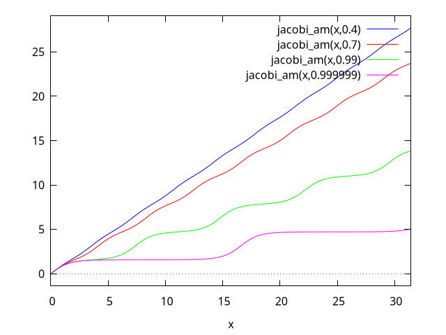
See also: jacobi_am, elliptic_f.
jacobi_cd (u, m) — Function
The Jacobian elliptic function ${\rm cd}(u,m) = {\rm cn}(u,m)/{\rm dn}(u,m).$
jacobi_cn (u, m) — Function
The Jacobian elliptic function ${\rm cn}(u,m).$
jacobi_cs (u, m) — Function
The Jacobian elliptic function ${\rm cs}(u,m) = {\rm cn}(u,m)/{\rm sn}(u,m).$
jacobi_dc (u, m) — Function
The Jacobian elliptic function ${\rm dc}(u,m) = {\rm dn}(u,m)/{\rm cn}(u,m).$
jacobi_dn (u, m) — Function
The Jacobian elliptic function ${\rm dn}(u,m).$
jacobi_ds (u, m) — Function
The Jacobian elliptic function ${\rm ds}(u,m) = {\rm dn}(u,m)/{\rm sn}(u,m).$
jacobi_nc (u, m) — Function
The Jacobian elliptic function ${\rm nc}(u,m) = 1/{\rm cn}(u,m).$
jacobi_nd (u, m) — Function
The Jacobian elliptic function ${\rm nd}(u,m) = 1/{\rm dn}(u,m).$
jacobi_ns (u, m) — Function
The Jacobian elliptic function ${\rm ns}(u,m) = 1/{\rm sn}(u,m).$
jacobi_sc (u, m) — Function
The Jacobian elliptic function ${\rm sc}(u,m) = {\rm sn}(u,m)/{\rm cn}(u,m).$
jacobi_sd (u, m) — Function
The Jacobian elliptic function ${\rm sd}(u,m) = {\rm sn}(u,m)/{\rm dn}(u,m).$
jacobi_sn (u, m) — Function
The Jacobian elliptic function ${\rm sn}(u,m).$
Special Functions
%f (p, q) — Function
The ${p}F{q}(a_1,a_2,…,a_p;b_1,b_2,…,b_q;z)$ hypergeometric function, where a a list of length p and b a list of length q.
%m (k, u) — Function
Whittaker M function (https://personal.math.ubc.ca/~cbm/aands/page_505.htmA&S eqn 13.1.32):
$$M_{\kappa,\mu}(z) = e^{-{1\over 2}z} z^{{1\over 2} + \mu} M\left({1\over 2} + \mu - \kappa, 1 + 2\mu, z\right)$$
$$M_{\kappa,\mu}(z) = e^{-{1\over 2}z} z^{{1\over 2} + \mu} M\left({1\over 2} + \mu - \kappa, 1 + 2\mu, z\right)$$
where $M(a,b,z)$ is Kummer’s solution of the confluent hypergeometric equation.
This can also be expressed by the series (https://dlmf.nist.gov/13.14.E6DLMF 13.14.E6):
$$M_{\kappa,\mu}(z) = e^{-{1\over 2} z} z^{{1\over 2} + \mu} \sum_{s=0}^{\infty} {\left({1\over 2} + \mu - \kappa\right)_s \over (1 + 2\mu)_s s!} z^s$$
$$M_{\kappa,\mu}(z) = e^{-{1\over 2} z} z^{{1\over 2} + \mu} \sum_{s=0}^{\infty} {\left({1\over 2} + \mu - \kappa\right)_s \over (1 + 2\mu)_s s!} z^s$$
%s (u, v) — Function
Lommel’s little
$s_{\mu,\nu}(z)$
function.
(https://dlmf.nist.gov/11.9.E3DLMF 11.9.E3)(G&R 8.570.1).
This Lommel function is the particular solution of the inhomogeneous Bessel differential equation:
$${d^2\over dz^2} + {1\over z}{dw\over dz} + \left(1-{\nu^2\over z^2}\right) w = z^{\mu-1}$$
$${d^2\over dz^2} + {1\over z}{dw\over dz} + \left(1-{\nu^2\over z^2}\right) w = z^{\mu-1}$$
This can be defined by the series
$$s_{\mu,\nu}(z) = z^{\mu+1}\sum_{k=0}^{\infty} (-1)^k {z^{2k}\over a_{k+1}(\mu, \nu)}$$
$$s_{\mu,\nu}(z) = z^{\mu+1}\sum_{k=0}^{\infty} (-1)^k {z^{2k}\over a_{k+1}(\mu, \nu)}$$
where
$$a_k(\mu,\nu) = \prod_{m=1}^k \left(\left(\mu + 2m-1\right)^2-\nu^2\right) = 4^k\left(\mu-\nu+1\over 2\right)_k \left(\mu+\nu+1\over 2\right)_k$$
$$a_k(\mu,\nu) = \prod_{m=1}^k \left(\left(\mu + 2m-1\right)^2-\nu^2\right) = 4^k\left(\mu-\nu+1\over 2\right)_k \left(\mu+\nu+1\over 2\right)_k$$
%w (k, u) — Function
Whittaker W function (https://personal.math.ubc.ca/~cbm/aands/page_505.htmA&S eqn 13.1.33):
$$W_{\kappa,\mu}(z) = e^{-{1\over 2}z} z^{{1\over 2} + \mu} U\left({1\over 2} + \mu - \kappa, 1+2\mu,z\right)$$
$$W_{\kappa,\mu}(z) = e^{-{1\over 2}z} z^{{1\over 2} + \mu} U\left({1\over 2} + \mu - \kappa, 1+2\mu,z\right)$$
where $U(a,b,z)$ is Kummer’s second solution of the confluent hypergeometric equation.
airy_ai (x) — Function
The Airy function ${\rm Ai}(x).$ See https://personal.math.ubc.ca/~cbm/aands/page_446.htmA&S eqn 10.4.2 and https://dlmf.nist.gov/9DLMF 9.
See also airy_bi, airy_dai, and airy_005fdbi.
See also: airy_bi, airy_dai, airy_dbi.
airy_bi (x) — Function
The Airy function ${\rm Bi}(x).$ See https://personal.math.ubc.ca/~cbm/aands/page_446.htmA&S eqn 10.4.3 and https://dlmf.nist.gov/9DLMF 9.
See airy_ai, and airy_005fdbi.
See also: airy_ai, airy_dbi.
airy_dai (x) — Function
The derivative of the Airy function ${\rm Ai}(x):$
$${\rm airy_dai}(x) = {d\over dx}{\rm Ai}(x)$$
$${\rm airy_dai}(x) = {d\over dx}{\rm Ai}(x)$$
See airy_005fai.
See also: airy_ai.
airy_dbi (x) — Function
The derivative of the Airy function ${\rm Bi}(x):$
$${\rm airy_dbi}(x) = {d\over dx}{\rm Bi}(x)$$
$${\rm airy_dbi}(x) = {d\over dx}{\rm Bi}(x)$$
See airy_ai, and airy_005fbi.
See also: airy_ai, airy_bi.
bessel_i (v, z) — Function
The modified Bessel function of the first kind of order $v$ and argument $z$. See https://personal.math.ubc.ca/~cbm/aands/page_375.htmA&S eqn 9.6.10 and https://dlmf.nist.gov/10.25.E2DLMF 10.25.E2.
bessel_i is defined as
$$I_v(z) = \sum_{k=0}^{\infty } {{1\over{k!,\Gamma \left(v+k+1\right)}} {\left(z\over 2\right)^{v+2,k}}}$$
$$I_v(z) = \sum_{k=0}^{\infty } {{1\over{k!,\Gamma \left(v+k+1\right)}} {\left(z\over 2\right)^{v+2,k}}}$$
although the infinite series is not used for computations.
When besselexpand is true, bessel_i is expanded in terms
of elementary functions when the order $v$ is half of an odd integer.
See besselexpand.
See also: bessel_i, besselexpand, true.
bessel_j (v, z) — Function
The Bessel function of the first kind of order $v$ and argument $z$. See https://personal.math.ubc.ca/~cbm/aands/page_360.htmA&S eqn 9.1.10 and https://dlmf.nist.gov/10.2.E2DLMF 10.2.E2.
bessel_j is defined as
$$J_v(z) = \sum_{k=0}^{\infty }{{{\left(-1\right)^{k},\left(z\over 2\right)^{v+2,k} }\over{k!,\Gamma\left(v+k+1\right)}}}$$
$$J_v(z) = \sum_{k=0}^{\infty }{{{\left(-1\right)^{k},\left(z\over 2\right)^{v+2,k} }\over{k!,\Gamma\left(v+k+1\right)}}}$$
although the infinite series is not used for computations.
When besselexpand is true, bessel_j is expanded in terms
of elementary functions when the order $v$ is half of an odd integer.
See besselexpand.
See also: bessel_j, besselexpand, true.
bessel_k (v, z) — Function
The modified Bessel function of the second kind of order $v$ and argument $z$. See https://personal.math.ubc.ca/~cbm/aands/page_375.htmA&S eqn 9.6.2 and https://dlmf.nist.gov/10.27.E4DLMF 10.27.E4.
bessel_k is defined as
$$K_v(z) = {1\over 2} \pi, {I_{-v}(z)-I_{v}(z) \over \sin v\pi}$$
$$K_v(z) = {1\over 2} \pi, {I_{-v}(z)-I_{v}(z) \over \sin v\pi}$$
when $v$ is not an integer. If $v$ is an integer $n$, then the limit as $v$ approaches $n$ is taken.
When besselexpand is true, bessel_k is expanded in terms
of elementary functions when the order $v$ is half of an odd integer.
See besselexpand.
See also: bessel_k, besselexpand, true.
bessel_y (v, z) — Function
The Bessel function of the second kind of order $v$ and argument $z$. See https://personal.math.ubc.ca/~cbm/aands/page_358.htmA&S eqn 9.1.2 and https://dlmf.nist.gov/10.2.E3DLMF 10.2.E3.
bessel_y is defined as
$$Y_v(z) = {{\cos(\pi v), J_v(z) - J_{-v}(z)}\over{\sin{\pi v}}}$$
$$Y_v(z) = {{\cos(\pi v), J_v(z) - J_{-v}(z)}\over{\sin{\pi v}}}$$
when $v$ is not an integer. When $v$ is an integer $n$, the limit as $v$ approaches $n$ is taken.
When besselexpand is true, bessel_y is expanded in terms
of elementary functions when the order $v$ is half of an odd integer.
See besselexpand.
See also: bessel_y, besselexpand, true.
besselexpand — Variable
Default value: false
Controls expansion of the Bessel, Hankel and Struve functions
when the order is half of
an odd integer. In this case, the functions can be expanded
in terms of other elementary functions. When besselexpand is true,
the Bessel function is expanded.
maxima
(%i1) besselexpand: false$
(%i2) bessel_j (3/2, z);
3
(%o2) bessel_j(-, z)
2
(%i3) besselexpand: true$
(%i4) bessel_j (3/2, z);
sin(z) cos(z)
sqrt(2) sqrt(z) (------ - ------)
2 z
z
(%o4) ---------------------------------
sqrt(%pi)
(%i5) bessel_y(3/2,z);
sin(z) cos(z)
sqrt(2) sqrt(z) (- ------ - ------)
z 2
z
(%o5) -----------------------------------
sqrt(%pi)
(%i6) bessel_i(3/2,z);
cosh(z) sinh(z)
sqrt(2) sqrt(z) (------- - -------)
z 2
z
(%o6) -----------------------------------
sqrt(%pi)
(%i7) bessel_k(3/2,z);
1 - z
sqrt(%pi) (- + 1) %e
z
(%o7) -----------------------
sqrt(2) sqrt(z)
See also: false, besselexpand, true.
beta (a, b) — Function
The beta function is defined as
$${\rm B}(a, b) = {{\Gamma(a) \Gamma(b)}\over{\Gamma(a+b)}}$$
$${\rm B}(a, b) = {{\Gamma(a) \Gamma(b)}\over{\Gamma(a+b)}}$$
(https://dlmf.nist.gov/5.12.E1DLMF 5.12.E1 and https://personal.math.ubc.ca/~cbm/aands/page_258.htmA&S eqn 6.2.1).
Maxima simplifies the beta function for positive integers and rational
numbers, which sum to an integer. When beta_args_sum_to_integer is
true, Maxima simplifies also general expressions which sum to an integer.
For a or b equal to zero the beta function is not defined.
In general the beta function is not defined for negative integers as an
argument. The exception is for a=-n, n a positive integer
and b a positive integer with b<=n, it is possible to define an
analytic continuation. Maxima gives for this case a result.
When beta_expand is true, expressions like beta and
beta or beta
and beta with n
an integer are simplified.
Maxima can evaluate the beta function for real and complex values in float and
bigfloat precision. For numerical evaluation Maxima uses log_gamma:
- log_gamma(b + a) + log_gamma(b) + log_gamma(a)
%e
Maxima knows that the beta function is symmetric and has mirror symmetry.
Maxima knows the derivatives of the beta function with respect to a or b.
To express the beta function as a ratio of gamma functions see makegamma.
Examples:
Simplification, when one of the arguments is an integer:
maxima
(%i1) [beta(2,3),beta(2,1/3),beta(2,a)];
1 9 1
(%o1) [--, -, ---------]
12 4 a (a + 1)
Simplification for two rational numbers as arguments which sum to an integer:
maxima
(%i1) [beta(1/2,5/2),beta(1/3,2/3),beta(1/4,3/4)];
3 %pi 2 %pi
(%o1) [-----, -------, sqrt(2) %pi]
8 sqrt(3)
When setting beta_args_sum_to_integer to true more general
expression are simplified, when the sum of the arguments is an integer:
maxima
(%i1) beta_args_sum_to_integer:true$
(%i2) beta(a+1,-a+2);
%pi (a - 1) a
(%o2) ------------------
2 sin(%pi (2 - a))
The possible results, when one of the arguments is a negative integer:
maxima
(%i1) [beta(-3,1),beta(-3,2),beta(-3,3)];
1 1 1
(%o1) [- -, -, - -]
3 6 3
beta or beta with n an integer simplifies when
beta_expand is true:
maxima
(%i1) beta_expand:true$
(%i2) [beta(a+1,b),beta(a-1,b),beta(a+1,b)/beta(a,b+1)];
a beta(a, b) beta(a, b) (b + a - 1) a
(%o2) [------------, ----------------------, -]
b + a a - 1 b
Beta is not defined, when one of the arguments is zero:
beta: expected nonzero arguments; found 0, b – an error. To debug this try: debugmode(true);
maxima
(%i1) beta(0,b);
Numerical evaluation for real and complex arguments in float or bigfloat precision:
maxima
(%i1) beta(2.5,2.3);
(%o1) 0.08694748611299981
(%i2) beta(2.5,1.4+%i);
(%o2) 0.06401449507966957 - 0.15020780532864159 %i
(%i3) beta(2.5b0,2.3b0);
(%o3) 8.694748611299965b-2
(%i4) beta(2.5b0,1.4b0+%i);
(%o4) 6.401449507966939b-2 - 1.502078053286414b-1 %i
Beta is symmetric and has mirror symmetry:
maxima
(%i1) beta(a,b)-beta(b,a);
(%o1) 0
(%i2) declare(a,complex,b,complex)$
(%i3) conjugate(beta(a,b));
(%o3) beta(conjugate(a), conjugate(b))
The derivative of the beta function wrt a:
maxima
(%i1) diff(beta(a,b),a);
(%o1) - beta(a, b) (psi (b + a) - psi (a))
0 0
See also: beta_args_sum_to_integer, true, beta_expand, beta, log_gamma, makegamma.
beta_args_sum_to_integer — Variable
Default value: false
When beta_args_sum_to_integer is true, Maxima simplifies
beta, when the arguments a and b sum to an integer.
beta for examples.
See also: beta_args_sum_to_integer, true, beta.
beta_expand — Variable
Default value: false
When beta_expand is true, beta and related
functions are expanded for arguments like $a+n$ or $a-n$,
where $n$ is an integer.
beta for examples.
See also: beta_expand, true, beta.
beta_incomplete (a, b, z) — Function
The basic definition of the incomplete beta function (https://dlmf.nist.gov/8.17.E1DLMF 8.17.E1 and https://personal.math.ubc.ca/~cbm/aands/page_263.htmA&S eqn 6.6.1) is
$${\rm B}_z(a,b) = \int_0^z t^{a-1}(1-t)^{b-1}; dt$$
$${\rm B}_z(a,b) = \int_0^z t^{a-1}(1-t)^{b-1}; dt$$
This definition is possible for ${\rm Re}(a) > 0$ and ${\rm Re}(b) > 0$ and $|z| < 1.$ For other values the incomplete beta function can be defined through a generalized hypergeometric function:
gamma(a) hypergeometric_generalized([a, 1 - b], [a + 1], z) z
(See https://functions.wolfram.com/GammaBetaErf/Beta3/ for a complete definition of the incomplete beta function.)
For negative integers $a = -n$ and positive integers $b=m$ with $m \le n$ the incomplete beta function is defined through
$$z^{n-1}\sum_{k=0}^{m-1} {{(1-m)_k z^k} \over {k! (n-k)}}$$
$$z^{n-1}\sum_{k=0}^{m-1} {{(1-m)_k z^k} \over {k! (n-k)}}$$
Maxima uses this definition to simplify beta_incomplete for a a
negative integer.
For a a positive integer, beta_incomplete simplifies for any
argument b and z and for b a positive integer for any
argument a and z, with the exception of a a negative integer.
For $z=0$ and
${\rm Re}(a) > 0,$
beta_incomplete has the
specific value zero. For $z=1$ and
${\rm Re}(b) > 0,$
beta_incomplete simplifies to the beta function beta.
Maxima evaluates beta_incomplete numerically for real and complex values
in float or bigfloat precision. For the numerical evaluation an expansion of the
incomplete beta function in continued fractions is used.
When the option variable beta_expand is true, Maxima expands
expressions like beta_005fincomplete and
beta_005fincomplete where $n$ is a positive integer.
Maxima knows the derivatives of beta_incomplete with respect to the
variables a, b and z and the integral with respect to the
variable z.
Examples:
Simplification for a a positive integer:
maxima
(%i1) beta_incomplete(2,b,z);
b
1 - (1 - z) (b z + 1)
(%o1) ----------------------
b (b + 1)
Simplification for b a positive integer:
maxima
(%i1) beta_incomplete(a,2,z);
a
(a (1 - z) + 1) z
(%o1) ------------------
a (a + 1)
Simplification for a and b a positive integer:
maxima
(%i1) beta_incomplete(3,2,z);
3
(3 (1 - z) + 1) z
(%o1) ------------------
12
a is a negative integer and $b\le -a$, Maxima simplifies:
maxima
(%i1) beta_incomplete(-3,1,z);
1
(%o1) - ----
3
3 z
For the specific values $z=0$ and $z=1$, Maxima simplifies:
maxima
(%i1) assume(a>0,b>0)$
(%i2) beta_incomplete(a,b,0);
(%o2) 0
(%i3) beta_incomplete(a,b,1);
(%o3) beta(a, b)
Numerical evaluation in float or bigfloat precision:
maxima
(%i1) beta_incomplete(0.25,0.50,0.9);
(%o1) 4.594959440269333
(%i2) fpprec:25$
(%i3) beta_incomplete(0.25,0.50,0.9b0);
(%o3) 4.594959440269324086971216b0
For $abs(z)>1$ beta_incomplete returns a complex result:
maxima
(%i1) beta_incomplete(0.25,0.50,1.7);
(%o1) 5.244115108584249 - 1.4551804778784403 %i
Results for more general complex arguments:
maxima
(%i1) beta_incomplete(0.25+%i,1.0+%i,1.7+%i);
(%o1) 2.7269606756625384 - 0.38311757042691896 %i
(%i2) beta_incomplete(1/2,5/4*%i,2.8+%i);
(%o2) 13.046496351687155 %i - 5.8020679562699975
Expansion, when beta_expand is true:
maxima
(%i1) beta_incomplete(a+1,b,z),beta_expand:true;
b a
a beta_incomplete(a, b, z) (1 - z) z
(%o1) -------------------------- - -----------
b + a b + a
(%i2) beta_incomplete(a-1,b,z),beta_expand:true;
b a - 1
beta_incomplete(a, b, z) (- b - a + 1) (1 - z) z
(%o2) -------------------------------------- - ---------------
1 - a 1 - a
Derivative and integral for beta_incomplete:
maxima
(%i1) diff(beta_incomplete(a, b, z), z);
b - 1 a - 1
(%o1) (1 - z) z
(%i2) integrate(beta_incomplete(a, b, z), z);
(%o2) beta_incomplete(a, b, z) z - beta_incomplete(a + 1, b, z)
(%i3) factor(diff(%, z));
(%o3) beta_incomplete(a, b, z)
See also: beta_incomplete, beta, beta_expand, true.
beta_incomplete_generalized (a, b, z1, z2) — Function
The basic definition of the generalized incomplete beta function is
$$\int_{z_1}^{z_2} t^{a-1}(1-t)^{b-1}; dt$$
$$\int_{z_1}^{z_2} t^{a-1}(1-t)^{b-1}; dt$$
Maxima simplifies beta_incomplete_regularized for a and b
a positive integer.
For
${\rm Re}(a) > 0$
and
$z_1 = 0$
or
$z_2 = 0,$
Maxima simplifies
beta_incomplete_generalized to beta_incomplete.
For
${\rm Re}(b) > 0$
and
$z_1 = 1$
or
$z_2 = 1,$
Maxima simplifies to an
expression with beta and beta_incomplete.
Maxima evaluates beta_incomplete_regularized for real and complex values
in float and bigfloat precision.
When beta_expand is true, Maxima expands
beta_incomplete_generalized for $a+n$ and $a-n$, n a
positive integer.
Maxima knows the derivative of beta_incomplete_generalized with respect
to the variables a, b, z1, and z2 and the integrals with
respect to the variables z1 and z2.
Examples:
Maxima simplifies beta_incomplete_generalized for a and b a
positive integer:
maxima
(%i1) beta_incomplete_generalized(2,b,z1,z2);
b b
(1 - z1) (b z1 + 1) - (1 - z2) (b z2 + 1)
(%o1) -------------------------------------------
b (b + 1)
(%i2) beta_incomplete_generalized(a,2,z1,z2);
a a
(a (1 - z2) + 1) z2 - (a (1 - z1) + 1) z1
(%o2) -------------------------------------------
a (a + 1)
(%i3) beta_incomplete_generalized(3,2,z1,z2);
2 2 2 2
(1 - z1) (3 z1 + 2 z1 + 1) - (1 - z2) (3 z2 + 2 z2 + 1)
(%o3) -----------------------------------------------------------
12
Simplification for specific values $z1=0$, $z2=0$, $z1=1$, or $z2=1$:
maxima
(%i1) assume(a > 0, b > 0)$
(%i2) beta_incomplete_generalized(a,b,z1,0);
(%o2) - beta_incomplete(a, b, z1)
(%i3) beta_incomplete_generalized(a,b,0,z2);
(%o3) - beta_incomplete(a, b, z2)
(%i4) beta_incomplete_generalized(a,b,z1,1);
(%o4) beta(a, b) - beta_incomplete(a, b, z1)
(%i5) beta_incomplete_generalized(a,b,1,z2);
(%o5) beta_incomplete(a, b, z2) - beta(a, b)
Numerical evaluation for real arguments in float or bigfloat precision:
maxima
(%i1) beta_incomplete_generalized(1/2,3/2,0.25,0.31);
(%o1) 0.09638178086368676
(%i2) fpprec:32$
(%i3) beta_incomplete_generalized(1/2,3/2,0.25,0.31b0);
(%o3) 9.6381780863686935309170054689964b-2
Numerical evaluation for complex arguments in float or bigfloat precision:
maxima
(%i1) beta_incomplete_generalized(1/2+%i,3/2+%i,0.25,0.31);
(%o1) - 0.09625463003205387 %i - 0.0033238477353540463
(%i2) fpprec:20$
(%i3) beta_incomplete_generalized(1/2+%i,3/2+%i,0.25,0.31b0);
(%o3) - 9.6254630032054178691b-2 %i - 3.3238477353543591914b-3
Expansion for $a+n$ or $a-n$, n a positive integer, when
beta_expand is true:
maxima
(%i1) beta_expand:true$
(%i2) beta_incomplete_generalized(a+1,b,z1,z2);
b a b a
(1 - z1) z1 - (1 - z2) z2
(%o2) -----------------------------
b + a
a beta_incomplete_generalized(a, b, z1, z2)
+ -------------------------------------------
b + a
(%i3) beta_incomplete_generalized(a-1,b,z1,z2);
beta_incomplete_generalized(a, b, z1, z2) (- b - a + 1)
(%o3) -------------------------------------------------------
1 - a
b a - 1 b a - 1
(1 - z2) z2 - (1 - z1) z1
- -------------------------------------
1 - a
Derivative wrt the variable z1 and integrals wrt z1 and z2:
maxima
(%i1) diff(beta_incomplete_generalized(a,b,z1,z2),z1);
b - 1 a - 1
(%o1) - (1 - z1) z1
(%i2) integrate(beta_incomplete_generalized(a,b,z1,z2),z1);
(%o2) beta_incomplete_generalized(a, b, z1, z2) z1
+ beta_incomplete(a + 1, b, z1)
(%i3) integrate(beta_incomplete_generalized(a,b,z1,z2),z2);
(%o3) beta_incomplete_generalized(a, b, z1, z2) z2
- beta_incomplete(a + 1, b, z2)
See also: beta_incomplete_regularized, beta_incomplete_generalized, beta_incomplete, beta, beta_expand, true.
beta_incomplete_regularized (a, b, z) — Function
The regularized incomplete beta function (https://dlmf.nist.gov/8.17.E2DLMF 8.17.E2 and https://personal.math.ubc.ca/~cbm/aands/page_263.htmA&S eqn 6.6.2), defined as
$$I_z(a,b) = {{\rm B}_z(a,b)\over {\rm B}(a,b)}$$
$$I_z(a,b) = {{\rm B}_z(a,b)\over {\rm B}(a,b)}$$
As for beta_incomplete this definition is not complete. See
https://functions.wolfram.com/GammaBetaErf/BetaRegularized/ for a complete definition of
beta_incomplete_regularized.
beta_incomplete_regularized simplifies a or b a positive
integer.
For $z=0$ and
${\rm Re}(a)>0,$
beta_incomplete_regularized has
the specific value 0. For $z=1$ and
${\rm Re}(b) > 0,$
beta_incomplete_regularized simplifies to 1.
Maxima can evaluate beta_incomplete_regularized for real and complex
arguments in float and bigfloat precision.
When beta_expand is true, Maxima expands
beta_incomplete_regularized for arguments $a+n$ or $a-n$,
where n is an integer.
Maxima knows the derivatives of beta_incomplete_regularized with respect
to the variables a, b, and z and the integral with respect to
the variable z.
Examples:
Simplification for a or b a positive integer:
maxima
(%i1) beta_incomplete_regularized(2,b,z);
b
(%o1) 1 - (1 - z) (b z + 1)
(%i2) beta_incomplete_regularized(a,2,z);
a
(%o2) (a (1 - z) + 1) z
(%i3) beta_incomplete_regularized(3,2,z);
3
(%o3) (3 (1 - z) + 1) z
For the specific values $z=0$ and $z=1$, Maxima simplifies:
maxima
(%i1) assume(a>0,b>0)$
(%i2) beta_incomplete_regularized(a,b,0);
(%o2) 0
(%i3) beta_incomplete_regularized(a,b,1);
(%o3) 1
Numerical evaluation for real and complex arguments in float and bigfloat precision:
maxima
(%i1) beta_incomplete_regularized(0.12,0.43,0.9);
(%o1) 0.9114011367359802
(%i2) fpprec:32$
(%i3) beta_incomplete_regularized(0.12,0.43,0.9b0);
(%o3) 9.1140113673598029169207248506439b-1
(%i4) beta_incomplete_regularized(1+%i,3/3,1.5*%i);
(%o4) 0.2865367499935405 %i - 0.12299596333468409
(%i5) fpprec:20$
(%i6) beta_incomplete_regularized(1+%i,3/3,1.5b0*%i);
(%o6) 2.8653674999354031589b-1 %i - 1.2299596333468401976b-1
Expansion, when beta_expand is true:
maxima
(%i1) beta_incomplete_regularized(a+1,b,z);
(%o1) beta_incomplete_regularized(a + 1, b, z)
(%i2) beta_incomplete_regularized(a-1,b,z);
(%o2) beta_incomplete_regularized(a - 1, b, z)
The derivative and the integral wrt z:
maxima
(%i1) diff(beta_incomplete_regularized(a,b,z),z);
b - 1 a - 1
(1 - z) z
(%o1) -------------------
beta(a, b)
(%i2) integrate(beta_incomplete_regularized(a,b,z),z);
(%o2) beta_incomplete_regularized(a, b, z) z
a beta_incomplete_regularized(a + 1, b, z)
- ------------------------------------------
b + a
See also: beta_incomplete, beta_incomplete_regularized, beta_expand, true.
bffac (expr, n) — Function
Bigfloat version of the factorial (shifted gamma) function. The second argument is how many digits to retain and return, it’s a good idea to request a couple of extra.
maxima
(%i1) bffac(1/2,16);
(%o1) 8.862269254527584b-1
(%i2) (1/2)!,numer;
(%o2) 0.886226925452758
(%i3) bffac(1/2,32);
(%o3) 8.862269254527580136490837416707b-1
bfpsi (n, z, fpprec) — Function
bfpsi is the polygamma function of real argument z and
integer order n. See polygamma for further
information. bfpsi0 is the digamma function.
bfpsi0 is equivalent to
bfpsi.
These functions return bigfloat values. fpprec is the bigfloat precision of the return value.
maxima
(%i1) bfpsi0(1/3, 15);
(%o1) - 3.13203378002081b0
(%i2) bfpsi0(1/3, 32);
(%o2) - 3.1320337800208063229964190742873b0
(%i3) bfpsi(0,1/3,32);
(%o3) - 3.1320337800208063229964190742873b0
(%i4) psi[0](1/3);
3 log(3) %pi
(%o4) - -------- - --------- - %gamma
2 2 sqrt(3)
(%i5) float(%);
(%o5) - 3.132033780020806
See also: bfpsi, polygamma, bfpsi0.
cbffac (z, fpprec) — Function
Complex bigfloat factorial.
load ("bffac") loads this function.
maxima
(%i1) cbffac(1+%i,16);
(%o1) 3.430658398165453b-1 %i + 6.529654964201666b-1
(%i2) (1+%i)!,numer;
(%o2) 0.3430658398165453 %i + 0.6529654964201667
erf (z) — Function
The Error Function erf(z):
$${\rm erf}\ z = {{2\over \sqrt{\pi}}} \int_0^z e^{-t^2}, dt$$
$${\rm erf}\ z = {{2\over \sqrt{\pi}}} \int_0^z e^{-t^2}, dt$$
(https://personal.math.ubc.ca/~cbm/aands/page_297.htmA&S eqn 7.1.1) and (https://dlmf.nist.gov/7.2.E1DLMF 7.2.E1).
See also flag erfflag. This can also be expressed in terms
of a hypergeometric function. hypergeometric_005frepresentation.
See also: erfflag, hypergeometric_representation.
erf_generalized (z1, z2) — Function
Generalized Error function Erf(z1,z2):
$${\rm erf}(z_1, z_2) = {{2\over \sqrt{\pi}}} \int_{z_1}^{z_2} e^{-t^2}, dt$$
$${\rm erf}(z_1, z_2) = {{2\over \sqrt{\pi}}} \int_{z_1}^{z_2} e^{-t^2}, dt$$
This can also be expressed in terms
of a hypergeometric function. hypergeometric_005frepresentation.
See also: hypergeometric_representation.
erf_representation — Variable
Default value: false
erf_representation controls how the error functions are
represented. It must be set to one of false, erf,
erfc, or erfi. When set to false, the error functions are not
modified. When set to erf, all error functions (erfc,
erfi, erf_generalized, fresnel_s and
fresnel_c) are converted to erf functions. Similarly,
erfc converts error functions to erfc. Finally
erfi converts the functions to erfi.
Converting to erf:
maxima
(%i1) erf_representation:erf;
(%o1) erf
(%i2) erfc(z);
(%o2) 1 - erf(z)
(%i3) erfi(z);
(%o3) - %i erf(%i z)
(%i4) erf_generalized(z1,z2);
(%o4) erf(z2) - erf(z1)
(%i5) fresnel_c(z);
sqrt(%pi) (%i + 1) z
(%o5) ((1 - %i) (erf(--------------------)
2
sqrt(%pi) (1 - %i) z
+ %i erf(--------------------)))/4
2
(%i6) fresnel_s(z);
sqrt(%pi) (%i + 1) z
(%o6) ((%i + 1) (erf(--------------------)
2
sqrt(%pi) (1 - %i) z
- %i erf(--------------------)))/4
2
Converting to erfc:
maxima
(%i1) erf_representation:erfc;
(%o1) erfc
(%i2) erf(z);
(%o2) 1 - erfc(z)
(%i3) erfc(z);
(%o3) erfc(z)
(%i4) erf_generalized(z1,z2);
(%o4) erfc(z1) - erfc(z2)
(%i5) fresnel_s(c);
sqrt(%pi) (%i + 1) c
(%o5) ((%i + 1) (- erfc(--------------------)
2
sqrt(%pi) (1 - %i) c
- %i (1 - erfc(--------------------)) + 1))/4
2
(%i6) fresnel_c(c);
sqrt(%pi) (%i + 1) c
(%o6) ((1 - %i) (- erfc(--------------------)
2
sqrt(%pi) (1 - %i) c
+ %i (1 - erfc(--------------------)) + 1))/4
2
Converting to erfc:
maxima
(%i1) erf_representation:erfi;
(%o1) erfi
(%i2) erf(z);
(%o2) - %i erfi(%i z)
(%i3) erfc(z);
(%o3) %i erfi(%i z) + 1
(%i4) erfi(z);
(%o4) erfi(z)
(%i5) erf_generalized(z1,z2);
(%o5) %i erfi(%i z1) - %i erfi(%i z2)
(%i6) fresnel_s(z);
sqrt(%pi) %i (%i + 1) z
(%o6) ((%i + 1) (- %i erfi(-----------------------)
2
sqrt(%pi) (1 - %i) %i z
- erfi(-----------------------)))/4
2
(%i7) fresnel_c(z);
sqrt(%pi) (1 - %i) %i z
(%o7) ((1 - %i) (erfi(-----------------------)
2
sqrt(%pi) %i (%i + 1) z
- %i erfi(-----------------------)))/4
2
See also: erf_representation, false, erf, erfc, erfi, erf_generalized, fresnel_s, fresnel_c.
erfc (z) — Function
The Complementary Error Function erfc(z):
$${\rm erfc}\ z = 1 - {\rm erf}\ z$$
$${\rm erfc}\ z = 1 - {\rm erf}\ z$$
(https://personal.math.ubc.ca/~cbm/aands/page_297.htmA&S eqn 7.1.2) and (https://dlmf.nist.gov/7.2.E2DLMF 7.2.E2).
This can also be expressed in terms
of a hypergeometric function. hypergeometric_005frepresentation.
See also: hypergeometric_representation.
erfi (z) — Function
The Imaginary Error Function.
$${\rm erfi}\ z = -i, {\rm erf}(i z)$$
$${\rm erfi}\ z = -i, {\rm erf}(i z)$$
expand_hypergeometric — Variable
Default value: false
When true, hypergeometric will return a polynomial if
the hypergeometric function represents a polynomial.
See also: false, true, hypergeometric.
fresnel_c (z) — Function
The Fresnel Integral
$$C(z) = \int_0^z \cos\left({\pi \over 2} t^2\right), dt$$
$$C(z) = \int_0^z \cos\left({\pi \over 2} t^2\right), dt$$
(https://personal.math.ubc.ca/~cbm/aands/page_300.htmA&S eqn 7.3.1) and (https://dlmf.nist.gov/7.2.E7DLMF 7.2.E7).
The simplification
$C(-x) = -C(x)$
is applied when
flag trigsign is true.
The simplification
$C(ix) = iC(x)$
is applied when
flag %iargs is true.
See flags erf_representation and hypergeometric_representation.
See also: trigsign, %iargs, erf_representation, hypergeometric_representation.
fresnel_s (z) — Function
The Fresnel Integral
$$S(z) = \int_0^z \sin\left({\pi \over 2} t^2\right), dt$$
$$S(z) = \int_0^z \sin\left({\pi \over 2} t^2\right), dt$$
(https://personal.math.ubc.ca/~cbm/aands/page_300.htmA&S eqn 7.3.2) and (https://dlmf.nist.gov/7.2.E8DLMF 7.2.E8).
The simplification
$S(-x) = -S(x)$
is applied when
flag trigsign is true.
The simplification
$S(ix) = iS(x)$
is applied when
flag %iargs is true.
See flags erf_representation and hypergeometric_representation.
See also: trigsign, %iargs, erf_representation, hypergeometric_representation.
gamma (z) — Function
The basic definition of the gamma function (https://dlmf.nist.gov/5.2.E1DLMF 5.2.E1 and https://personal.math.ubc.ca/~cbm/aands/page_255.htmA&S eqn 6.1.1) is
$$\Gamma\left(z\right)=\int_{0}^{\infty }{t^{z-1},e^ {- t };dt}$$
$$\Gamma\left(z\right)=\int_{0}^{\infty }{t^{z-1},e^ {- t };dt}$$
Maxima simplifies gamma for positive integer and positive and negative
rational numbers. For half integral values the result is a rational number
times
$\sqrt{\pi}.$
The simplification for integer values is controlled by
factlim. For integers greater than factlim the numerical result of
the factorial function, which is used to calculate gamma, will overflow.
The simplification for rational numbers is controlled by gammalim to
avoid internal overflow. See factlim and gammalim.
For negative integers gamma is not defined.
Maxima can evaluate gamma numerically for real and complex values in float
and bigfloat precision.
gamma has mirror symmetry.
When gamma_expand is true, Maxima expands gamma for
arguments z+n and z-n where n is an integer.
Maxima knows the derivative of gamma.
Examples:
Simplification for integer, half integral, and rational numbers:
maxima
(%i1) map('gamma,[1,2,3,4,5,6,7,8,9]);
(%o1) [1, 1, 2, 6, 24, 120, 720, 5040, 40320]
(%i2) map('gamma,[1/2,3/2,5/2,7/2]);
sqrt(%pi) 3 sqrt(%pi) 15 sqrt(%pi)
(%o2) [sqrt(%pi), ---------, -----------, ------------]
2 4 8
(%i3) map('gamma,[2/3,5/3,7/3]);
2 1
2 gamma(-) 4 gamma(-)
2 3 3
(%o3) [gamma(-), ----------, ----------]
3 3 9
Numerical evaluation for real and complex values:
maxima
(%i1) map('gamma,[2.5,2.5b0]);
(%o1) [1.329340388179137, 1.329340388179137b0]
(%i2) map('gamma,[1.0+%i,1.0b0+%i]);
(%o2) [0.49801566811835596 - 0.15494982830181073 %i,
4.980156681183561b-1 - 1.549498283018107b-1 %i]
gamma has mirror symmetry:
maxima
(%i1) declare(z,complex)$
(%i2) conjugate(gamma(z));
(%o2) gamma(conjugate(z))
Maxima expands gamma and gamma, when gamma_expand
is true:
maxima
(%i1) gamma_expand:true$
(%i2) [gamma(z+1),gamma(z-1),gamma(z+2)/gamma(z+1)];
gamma(z)
(%o2) [z gamma(z), --------, z + 1]
z - 1
The derivative of gamma:
maxima
(%i1) diff(gamma(z),z);
(%o1) psi (z) gamma(z)
0
See also makegamma.
The Euler-Mascheroni constant is %gamma.
See also: gamma, factlim, gammalim, gamma_expand, true, makegamma, %gamma.
gamma_expand — Variable
Default value: false
gamma_expand controls expansion of gamma_incomplete.
When gamma_expand is true, gamma_005fincomplete
is expanded in terms of
z, exp, and gamma_incomplete or erfc when possible.
maxima
(%i1) gamma_incomplete(2,z);
(%o1) gamma_incomplete(2, z)
(%i2) gamma_expand:true;
(%o2) true
(%i3) gamma_incomplete(2,z);
- z
(%o3) (z + 1) %e
(%i4) gamma_incomplete(3/2,z);
- z sqrt(%pi) erfc(sqrt(z))
(%o4) sqrt(z) %e + -----------------------
2
(%i5) gamma_incomplete(4/3,z);
1
gamma_incomplete(-, z)
1/3 - z 3
(%o5) z %e + ----------------------
3
(%i6) gamma_incomplete(a+2,z);
a - z
(%o6) z (z + a + 1) %e + a (a + 1) gamma_incomplete(a, z)
(%i7) gamma_incomplete(a-2, z);
gamma_incomplete(a, z) a - 2 z 1
(%o7) ---------------------- - z (--------------- + -----)
(1 - a) (2 - a) (a - 2) (a - 1) a - 2
- z
%e
See also: false, gamma_expand, gamma_incomplete, true, exp, erfc.
gamma_incomplete (a, z) — Function
The incomplete upper gamma function (https://dlmf.nist.gov/8.2.E2DLMF 8.2.E2 and https://personal.math.ubc.ca/~cbm/aands/page_260.htmA&S eqn 6.5.3):
$$\Gamma\left(a , z\right)=\int_{z}^{\infty }{t^{a-1},e^ {- t };dt}$$
$$\Gamma\left(a , z\right)=\int_{z}^{\infty }{t^{a-1},e^ {- t };dt}$$
See also gamma_expand for controlling how
gamma_incomplete is expressed in terms of elementary functions
and erfc.
Also see the related functions gamma_incomplete_regularized and
gamma_incomplete_generalized.
See also: gamma_expand, gamma_incomplete, erfc, gamma_incomplete_regularized, gamma_incomplete_generalized.
gamma_incomplete_generalized (a, z1, z1) — Function
The generalized incomplete gamma function.
$$\Gamma\left(a , z_{1}, z_{2}\right)=\int_{z_{1}}^{z_{2}}{t^{a-1},e^ {- t };dt}$$
$$\Gamma\left(a , z_{1}, z_{2}\right)=\int_{z_{1}}^{z_{2}}{t^{a-1},e^ {- t };dt}$$
Also see gamma_incomplete and gamma_incomplete_regularized.
See also: gamma_incomplete, gamma_incomplete_regularized.
gamma_incomplete_lower (a, z) — Function
The lower incomplete gamma function (https://dlmf.nist.gov/8.2.E1DLMF 8.2.E1 and https://personal.math.ubc.ca/~cbm/aands/page_260.htmA&S eqn 6.5.2):
$$\gamma\left(a , z\right)=\int_{0}^{z}{t^{a-1},e^ {- t };dt}$$
$$\gamma\left(a , z\right)=\int_{0}^{z}{t^{a-1},e^ {- t };dt}$$
See also gamma_incomplete (upper incomplete gamma function).
See also: gamma_incomplete.
gamma_incomplete_regularized (a, z) — Function
The regularized incomplete upper gamma function (https://dlmf.nist.gov/8.2.E4DLMF 8.2.E4):
$$Q\left(a , z\right)={{\Gamma\left(a , z\right)}\over{\Gamma\left(a\right)}}$$
$$Q\left(a , z\right)={{\Gamma\left(a , z\right)}\over{\Gamma\left(a\right)}}$$
See also gamma_expand for controlling how
gamma_incomplete is expressed in terms of elementary functions
and erfc.
Also see gamma_incomplete.
See also: gamma_expand, gamma_incomplete, erfc.
gammalim — Variable
Default value: 10000
gammalim controls simplification of the gamma
function for integral and rational number arguments. If the absolute
value of the argument is not greater than gammalim, then
simplification will occur. Note that the factlim switch controls
simplification of the result of gamma of an integer argument as well.
See also: gammalim, factlim, gamma.
generalized_lambert_w (k, z) — Function
The k-th branch of Lambert’s W function W(z) (https://dlmf.nist.gov/4.13DLMF 4.13), the solution of $z=W(z)e^{W(z)}.$
The principal branch, denoted
$W_p(z)$
in DLMF, is lambert_005fw =
generalized_005flambert_005fw.
The other branch with real values, denoted
$W_m(z)$
in DLMF, is generalized_005flambert_005fw.
See also: lambert_w, generalized_lambert_w.
hankel_1 (v, z) — Function
The Hankel function of the first kind of order $v$ and argument $z$. See https://personal.math.ubc.ca/~cbm/aands/page_358.htmA&S eqn 9.1.3 and https://dlmf.nist.gov/10.4.E3DLMF 10.4.E3.
hankel_1 is defined as
$$H^{(1)}_v(z) = J_v(z) + i Y_v(z)$$
$$H^{(1)}_v(z) = J_v(z) + i Y_v(z)$$
Maxima evaluates hankel_1 numerically for a complex order $v$ and
complex argument $z$ in float precision. The numerical evaluation in
bigfloat precision is not supported.
When besselexpand is true, hankel_1 is expanded in terms
of elementary functions when the order $v$ is half of an odd integer.
See besselexpand.
Maxima knows the derivative of hankel_1 wrt the argument $z$.
Examples:
Numerical evaluation:
maxima
(%i1) hankel_1(1,0.5);
(%o1) 0.24226845767487384 - 1.4714723926702433 %i
(%i2) hankel_1(1,0.5+%i);
(%o2) - 0.2558287994862166 %i - 0.23957560188301597
Expansion of hankel_1 when besselexpand is true:
maxima
(%i1) hankel_1(1/2,z),besselexpand:true;
sqrt(2) sin(z) - sqrt(2) %i cos(z)
(%o1) ----------------------------------
sqrt(%pi) sqrt(z)
Derivative of hankel_1 wrt the argument $z$. The derivative wrt the
order $v$ is not supported. Maxima returns a noun form:
maxima
(%i1) diff(hankel_1(v,z),z);
hankel_1(v - 1, z) - hankel_1(v + 1, z)
(%o1) ---------------------------------------
2
(%i2) diff(hankel_1(v,z),v);
d
(%o2) -- (hankel_1(v, z))
dv
See also: hankel_1, besselexpand, true.
hankel_2 (v, z) — Function
The Hankel function of the second kind of order $v$ and argument $z$. See https://personal.math.ubc.ca/~cbm/aands/page_358.htmA&S eqn 9.1.4 and https://dlmf.nist.gov/10.4.E3DLMF 10.4.E3.
hankel_2 is defined as
$$H^{(2)}_v(z) = J_v(z) - i Y_v(z)$$
$$H^{(2)}_v(z) = J_v(z) - i Y_v(z)$$
Maxima evaluates hankel_2 numerically for a complex order $v$ and
complex argument $z$ in float precision. The numerical evaluation in
bigfloat precision is not supported.
When besselexpand is true, hankel_2 is expanded in terms
of elementary functions when the order $v$ is half of an odd integer.
See besselexpand.
Maxima knows the derivative of hankel_2 wrt the argument $z$.
For examples see hankel_1.
See also: hankel_2, besselexpand, true, hankel_1.
hgfred (a, b, t) — Function
Simplify the generalized hypergeometric function in terms of other, simpler, forms. a is a list of numerator parameters and b is a list of the denominator parameters.
If hgfred cannot simplify the hypergeometric function, it returns
an expression of the form _0025f where p is
the number of elements in a, and q is the number of elements
in b. This is the usual
$_pF_q$
generalized hypergeometric
function.
maxima
(%i1) assume(not(equal(z,0)));
(%o1) [notequal(z, 0)]
(%i2) hgfred([v+1/2],[2*v+1],2*%i*z);
v/2 %i z
4 bessel_j(v, z) gamma(v + 1) %e
(%o2) ---------------------------------------
v
z
(%i3) hgfred([1,1],[2],z);
log(1 - z)
(%o3) - ----------
z
(%i4) hgfred([a,a+1/2],[3/2],z^2);
1 - 2 a 1 - 2 a
(z + 1) - (1 - z)
(%o4) -------------------------------
2 (1 - 2 a) z
It can be beneficial to load orthopoly too as the following example shows. Note that L is the generalized Laguerre polynomial.
maxima
(%i1) load("orthopoly")$
(%i2) hgfred([-2],[a],z);
2
z 2 z
(%o2) --------- - --- + 1
a (a + 1) a
(%i3) ev(%);
2
z 2 z
(%o3) --------- - --- + 1
a (a + 1) a
See also: hgfred, %f.
hypergeometric ([a1, …, ap], [b1, …, bq], x) — Function
The hypergeometric function. Unlike Maxima’s %f hypergeometric
function, the function hypergeometric is a simplifying
function; also, hypergeometric supports complex double and
big floating point evaluation. For the Gauss hypergeometric function,
that is $p = 2$ and $q = 1$, floating point evaluation
outside the unit circle is supported, but in general, it is not
supported.
When the option variable expand_hypergeometric is true (default
is false) and one of the arguments a1 through ap is a
negative integer (a polynomial case), hypergeometric returns an
expanded polynomial.
Examples:
maxima
(%i1) hypergeometric([],[],x);
x
(%o1) %e
Polynomial cases automatically expand when expand_hypergeometric is true:
maxima
(%i1) hypergeometric([-3],[7],x);
(%o1) hypergeometric([- 3], [7], x)
(%i2) hypergeometric([-3],[7],x), expand_hypergeometric : true;
3 2
x 3 x 3 x
(%o2) - --- + ---- - --- + 1
504 56 7
Both double float and big float evaluation is supported:
maxima
(%i1) hypergeometric([5.1],[7.1 + %i],0.42);
(%o1) 1.3462507863753337 - 0.0559061414208204 %i
(%i2) hypergeometric([5,6],[8], 5.7 - %i);
(%o2) 0.007375824009774945 - 0.0010498136885786736 %i
(%i3) hypergeometric([5,6],[8], 5.7b0 - %i), fpprec : 30;
(%o3) 7.37582400977494674506442010824b-3
- 1.04981368857867315858055393376b-3 %i
See also: %f, hypergeometric, expand_hypergeometric, true, false.
hypergeometric_representation — Variable
Default value: false
Enables transformation to a Hypergeometric
representation for fresnel_s and fresnel_c and other
error functions.
maxima
(%i1) hypergeometric_representation:true;
(%o1) true
(%i2) fresnel_s(z);
2 4
3 3 7 %pi z 3
%pi hypergeometric([-], [-, -], - -------) z
4 2 4 16
(%o2) ---------------------------------------------
6
(%i3) fresnel_c(z);
2 4
1 1 5 %pi z
(%o3) hypergeometric([-], [-, -], - -------) z
4 2 4 16
(%i4) erf(z);
2
3 2 - z
2 hypergeometric([1], [-], z ) z %e
2
(%o4) ---------------------------------------
sqrt(%pi)
(%i5) erfi(z);
1 3 2
2 hypergeometric([-], [-], z ) z
2 2
(%o5) --------------------------------
sqrt(%pi)
(%i6) erfc(z);
2
3 2 - z
2 hypergeometric([1], [-], z ) z %e
2
(%o6) 1 - ---------------------------------------
sqrt(%pi)
(%i7) erf_generalized(z1,z2);
2
3 2 - z2
2 hypergeometric([1], [-], z2 ) z2 %e
2
(%o7) ------------------------------------------
sqrt(%pi)
2
3 2 - z1
2 hypergeometric([1], [-], z1 ) z1 %e
2
- ------------------------------------------
sqrt(%pi)
See also: fresnel_s, fresnel_c.
hypergeometric_simp (e) — Function
hypergeometric_simp simplifies hypergeometric functions
by applying hgfred
to the arguments of any hypergeometric functions in the expression e.
Only instances of hypergeometric are affected;
any %f, %w, and %m in the expression e are not affected.
Any unsimplified hypergeometric functions are returned unchanged
(instead of changing to %f as hgfred would).
load("hypergeometric"); loads this function.
See also hgfred.
Examples:
maxima
(%i1) load ("hypergeometric") $
(%i2) foo : [hypergeometric([1,1], [2], z), hypergeometric([1/2], [1], z)];
(%o2) [hypergeometric([1, 1], [2], z),
1
hypergeometric([-], [1], z)]
2
(%i3) hypergeometric_simp (foo);
log(1 - z) z/2 z
(%o3) [- ----------, %e bessel_i(0, -)]
z 2
(%i4) bar : hypergeometric([n], [m], z + 1);
(%o4) hypergeometric([n], [m], z + 1)
(%i5) hypergeometric_simp (bar);
(%o5) hypergeometric([n], [m], z + 1)
See also: hypergeometric_simp, hgfred, hypergeometric, %f, %w, %m.
kbateman (v) — Function
The Bateman k function
$$k_v(x) = \frac{2}{\pi} \int_0^{\pi/2} \cos(x \tan\theta-v\theta)d\theta$$
$$k_v(x) = \frac{2}{\pi} \int_0^{\pi/2} \cos(x \tan\theta-v\theta)d\theta$$
It is one solution of a differential equation which appears in the theory of turbulence:
$$x {d^2u\over dx^2} = (x-\nu)u$$
$$x {d^2u\over dx^2} = (x-\nu)u$$
It is a special case of the confluent hypergeometric function for $x > 0$:
$$k_v(x) = {e^{-x}\over{\Gamma\left(1+{1\over 2}\nu\right)}} U\left(-{1\over 2} \nu, 0, 2x\right)$$
$$k_v(x) = {e^{-x}\over{\Gamma\left(1+{1\over 2}\nu\right)}} U\left(-{1\over 2} \nu, 0, 2x\right)$$
where $U$ is the confluent hypergeometric function. Also, we have
$$k_{2\nu}(z) = {1\over\Gamma(\nu+1)} W_{\nu,1/2}(2z)$$
$$k_{2\nu}(z) = {1\over\Gamma(\nu+1)} W_{\nu,1/2}(2z)$$
where
$W$
is the _0025w.
Some examples:
(%i1) assume(x > 0)$
(%i2) makelist(kbateman[n](0),n,0,5);
2 2 2
(%o2) [0, ---, 0, - -----, 0, -----]
%pi 3 %pi 5 %pi
(%i3) kbateman[0](x);
- x
(%o3) %e
(%i4) kbateman[2](x);
- x
(%o4) 2 %e x
(%i5) kbateman[4](x);
- x
(%o5) 2 %e (x - 1) x
(%i6) kbateman[3](x);
(%o6) kbateman (x)
3
Maxima can
calculate the Laplace transform of kbateman using laplace
or specint, as shown below:
(%i1) assume(s>0)$
(%i2) specint(kbateman[v](z)*exp(-s*z),z);
v v s - 1
2 %f ([2, 1 - -], [2 - -], -----)
2, 1 2 2 s + 1
(%o2) ------------------------------------
2 v v
(s + 1) gamma(2 - -) gamma(- + 1)
2 2
See also: %w, kbateman, laplace, specint.
lambert_w (z) — Function
The principal branch of Lambert’s W function W(z) (https://dlmf.nist.gov/4.13DLMF 4.13), the solution of
$$z = W(z)e^{W(z)}$$
$$z = W(z)e^{W(z)}$$
log_gamma (z) — Function
The natural logarithm of the gamma function.
maxima
(%i1) gamma(6);
(%o1) 120
(%i2) log_gamma(6);
(%o2) log(120)
(%i3) log_gamma(0.5);
(%o3) 0.5723649429247004
makefact (expr) — Function
Transforms instances of binomial, gamma, and beta functions in expr into factorials.
See also makegamma.
maxima
(%i1) makefact(binomial(n,k));
n!
(%o1) -----------
k! (n - k)!
(%i2) makefact(gamma(x));
(%o2) (x - 1)!
(%i3) makefact(beta(a,b));
(a - 1)! (b - 1)!
(%o3) -----------------
(b + a - 1)!
See also: makegamma.
makegamma (expr) — Function
Transforms instances of binomial, factorial, and beta functions in expr into gamma functions.
See also makefact.
maxima
(%i1) makegamma(binomial(n,k));
gamma(n + 1)
(%o1) -----------------------------
gamma(k + 1) gamma(n - k + 1)
(%i2) makegamma(x!);
(%o2) gamma(x + 1)
(%i3) makegamma(beta(a,b));
gamma(a) gamma(b)
(%o3) -----------------
gamma(b + a)
See also: makefact.
maxpsifracdenom — Variable
Default value: 6
Let $x$ be a rational number of the form $p/q$.
If $q$ is greater than maxpsifracdenom,
then
$\psi^{(0)}(x)$
will
not try to return a simplified value.
maxima
(%i1) psi[0](3/4);
%pi
(%o1) - 3 log(2) + --- - %gamma
2
(%i2) psi[2](3/4);
1 3
(%o2) psi (-) + 4 %pi
2 4
(%i3) maxpsifracdenom:2;
(%o3) 2
(%i4) psi[0](3/4);
3
(%o4) psi (-)
0 4
(%i5) psi[2](3/4);
1 3
(%o5) psi (-) + 4 %pi
2 4
See also: maxpsifracdenom.
maxpsifracnum — Variable
Default value: 6
Let $x$ be a rational number of the form $p/q$.
If $p$ is greater than maxpsifracnum,
then
$\psi^{(0)}(x)$
will not try to
return a simplified value.
maxima
(%i1) psi[0](3/4);
%pi
(%o1) - 3 log(2) + --- - %gamma
2
(%i2) psi[2](3/4);
1 3
(%o2) psi (-) + 4 %pi
2 4
(%i3) maxpsifracnum:2;
(%o3) 2
(%i4) psi[0](3/4);
3
(%o4) psi (-)
0 4
(%i5) psi[2](3/4);
1 3
(%o5) psi (-) + 4 %pi
2 4
See also: maxpsifracnum.
maxpsinegint — Variable
Default value: -10
maxpsinegint is the most negative value for
which
$\psi^{(0)}(x)$
will try to compute an exact
value for rational $x$. That is if $x$ is less than
maxpsinegint,
$\psi^{(n)}(x)$
will not
return simplified answer, even if it could.
maxima
(%i1) psi[0](-100/9);
100
(%o1) psi (- ---)
0 9
(%i2) psi[0](-100/11);
100 %pi 1 5231385863539
(%o2) %pi cot(-------) + psi (--) + -------------
11 0 11 381905105400
(%i3) psi[2](-100/9);
100
(%o3) psi (- ---)
2 9
(%i4) psi[2](-100/11);
3 100 %pi 2 100 %pi 1
(%o4) 2 %pi cot(-------) csc (-------) + psi (--)
11 11 2 11
74191313259470963498957651385614962459
+ --------------------------------------
27850718060013605318710152732000000
See also: maxpsinegint.
maxpsiposint — Variable
Default value: 20
maxpsiposint is the largest positive integer value for
which
$\psi^{(n)}(m)$
gives an exact value for
rational $x$.
maxima
(%i1) psi[0](20);
275295799
(%o1) --------- - %gamma
77597520
(%i2) psi[0](21);
(%o2) psi (21)
0
(%i3) psi[2](20);
1683118856778495358491487
(%o3) 2 (------------------------- - zeta(3))
1401731326612193601024000
(%i4) psi[2](21);
(%o4) psi (21)
2
See also: maxpsiposint.
numfactor (expr) — Function
Returns the numerical factor multiplying the expression expr, which should be a single term.
content returns the greatest common divisor (gcd) of all terms in a sum.
maxima
(%i1) gamma (7/2);
15 sqrt(%pi)
(%o1) ------------
8
(%i2) numfactor (%);
15
(%o2) --
8
See also: content.
nzeta (z) — Function
The Plasma Dispersion Function
$${\rm nzeta}(z) = i\sqrt{\pi}e^{-z^2}(1-{\rm erf}(-iz))$$
$${\rm nzeta}(z) = i\sqrt{\pi}e^{-z^2}(1-{\rm erf}(-iz))$$
nzetai (z) — Function
Returns imagpart(nzeta(z)).
nzetar (z) — Function
Returns realpart(nzeta(z)).
parabolic_cylinder_d (v, z) — Function
The parabolic cylinder function parabolic_005fcylinder_005fd. (https://personal.math.ubc.ca/~cbm/aands/page_687.htmA&S eqn 19.3.1).
The solution of the Weber differential equation
$$y’’(z) + \left(\nu + {1\over 2} - {1\over 4} z^2\right) y(z) = 0$$
$$y’’(z) + \left(\nu + {1\over 2} - {1\over 4} z^2\right) y(z) = 0$$
has two independent solutions, one of which is $D_{\nu}(z),$ the parabolic cylinder d function.
Function specint can return expressions containing
parabolic_005fcylinder_005fd if the option variable
prefer_d is true.
See also: parabolic_cylinder_d, specint, prefer_d, true.
psi (n) — Function
psi is the polygamma function (https://dlmf.nist.gov/5.2E2DLMF 5.2E2,
https://dlmf.nist.gov/5.15DLMF 5.15, https://personal.math.ubc.ca/~cbm/aands/page_258.htmA&S eqn 6.3.1 and https://personal.math.ubc.ca/~cbm/aands/page_260.htmA&S eqn 6.4.1) defined by
$$\psi^{(n)}(x) = {d^{n+1}\over{dx^{n+1}}} \log\Gamma(x)$$
$$\psi^{(n)}(x) = {d^{n+1}\over{dx^{n+1}}} \log\Gamma(x)$$
Thus, psi is the first derivative,
psi is the second derivative, etc.
Maxima can compute some exact values for rational args as well for
float and bfloat args. Several variables control what range of
rational args
$\psi^{(n)}(x)$
will return an
exact value, if possible. See maxpsiposint,
maxpsinegint, maxpsifracnum, and
maxpsifracdenom. That is, $x$ must lie between
maxpsinegint and maxpsiposint. If the absolute value of
the fractional part of $x$ is rational and has a numerator less
than maxpsifracnum and has a denominator less than
maxpsifracdenom,
$\psi^{(0)}(x)$
will
return an exact value.
The function bfpsi in the bffac package can compute
numerical values.
maxima
(%i1) psi[0](.25);
(%o1) - 4.227453533376265
(%i2) psi[0](1/4);
%pi
(%o2) - 3 log(2) - --- - %gamma
2
(%i3) float(%);
(%o3) - 4.227453533376265
(%i4) psi[2](0.75);
(%o4) - 5.3026332163376395
(%i5) psi[2](3/4);
1 3
(%o5) psi (-) + 4 %pi
2 4
(%i6) float(%);
(%o6) - 5.3026332163376395
See also: psi, maxpsiposint, maxpsinegint, maxpsifracnum, maxpsifracdenom, bfpsi, bffac.
scaled_bessel_i (v, z) — Function
The scaled modified Bessel function of the first kind of order $v$ and argument $z$. That is,
$${\rm scaled_bessel_i}(v,z) = e^{-|z|} I_v(z).$$
$${\rm scaled_bessel_i}(v,z) = e^{-|z|} I_v(z).$$
This function is particularly useful
for calculating
$I_v(z)$
for large $z$, which is large.
However, maxima does not otherwise know much about this function. For
symbolic work, it is probably preferable to work with the expression
exp(-abs(z))*bessel_i(v, z).
scaled_bessel_i0 (z) — Function
Identical to scaled_005fbessel_005fi.
See also: scaled_bessel_i.
scaled_bessel_i1 (z) — Function
Identical to scaled_005fbessel_005fi.
See also: scaled_bessel_i.
sinc (x) — Function
The function sinc is defined by
$${\rm sinc}(x) = \left@{ \matrix{ \displaystyle{\frac{\sin x}{x}} & {\rm if}> x \neq 0\cr & \cr % For extra vertical space 1 & {\rm if}> x = 0 } \right.$$
$${\rm sinc}(x) = \left@{ \matrix{ \displaystyle{\frac{\sin x}{x}} & {\rm if}> x \neq 0\cr & \cr % For extra vertical space 1 & {\rm if}> x = 0 } \right. $$
making sinc continuous at zero. The definition used here is the unnormalized version of the sinc
function.
When %piargs is true (the default),
${\rm sinc}(x)$
evaluates to an exact value when $x$ is an
explicit integer multiple of
$\pi,$
$\pi/4,$
or
$\pi/6.$
For other nonzero symbolic arguments,
sinc does not simplify to
$\sin(x)/x.$
For real or complex floating-point arguments (double or big floats), sinc returns a floating-point
value in rectangular form. When numer is true, sinc returns a floating-point value in rectangular
form for all numeric arguments, including rational numbers and big float numbers.
maxima
(%i1) sinc(%pi);
(%o1) 0
(%i2) %piargs : false$
(%i3) sinc(pi);
(%o3) sinc(pi)
(%i4) sinc(1.0 + 5.0*%i);
(%o4) 10.111782590680328 - 10.466747175403242 %i
(%i5) sinc(1 + 5*%i);
(%o5) sinc(5 %i + 1)
(%i6) sinc(1 + 5*%i), numer;
(%o6) 10.111782590680328 - 10.466747175403242 %i
(%i7) sinc(1.2b0 + 5.6b0*%i), numer;
(%o7) 12.975676863468047 - 19.724089614291696 %i
See also: sinc, %piargs, numer.
slommel (u, v) — Function
Lommel’s big
$S_{\mu,\nu}(z)$
function.
(https://dlmf.nist.gov/11.9.E5DLMF 11.9.E5)(G&R 8.570.2).
Lommels big S function is another particular solution of the
inhomogeneous Bessel differential equation
(_0025s) defined for all values
of
$\mu$
and
$\nu,$
where
$$\eqalign{ S_{\mu,\nu}(z) = s_{\mu,\nu}(z) + 2^{\mu-1} & \Gamma\left({\mu\over 2} + {\nu\over 2} + {1\over 2}\right) \Gamma\left({\mu\over 2} - {\nu\over 2} + {1\over 2}\right) \cr & \times \left(\sin\left({(\mu-\nu)\pi\over 2}\right) J_{\nu}(z) - \cos\left({(\mu-\nu)\pi\over 2}\right) Y_{\nu}(z)\right) }$$
$$\eqalign{ S_{\mu,\nu}(z) = s_{\mu,\nu}(z) + 2^{\mu-1} & \Gamma\left({\mu\over 2} + {\nu\over 2} + {1\over 2}\right) \Gamma\left({\mu\over 2} - {\nu\over 2} + {1\over 2}\right) \cr & \times \left(\sin\left({(\mu-\nu)\pi\over 2}\right) J_{\nu}(z) - \cos\left({(\mu-\nu)\pi\over 2}\right) Y_{\nu}(z)\right) }$$
When $\mu\pm \nu$ is an odd negative integer, the limit must be used.
See also: %s.
struve_h (v, z) — Function
The Struve Function H of order $\nu$ and argument $z$:
$${\bf H}{\nu}(z) = \left({z\over 2}\right)^{\nu+1} \sum{k=0}^{\infty} {(-1)^k\left({z\over 2}\right)^{2k} \over \Gamma\left(k + {3\over 2}\right) \Gamma\left(k + \nu + {3\over 2}\right)}$$
$${\bf H}{\nu}(z) = \left({z\over 2}\right)^{\nu+1} \sum{k=0}^{\infty} {(-1)^k\left({z\over 2}\right)^{2k} \over \Gamma\left(k + {3\over 2}\right) \Gamma\left(k + \nu + {3\over 2}\right)}$$
(https://personal.math.ubc.ca/~cbm/aands/page_496.htmA&S eqn 12.1.3) and (https://dlmf.nist.gov/11.2.E1DLMF 11.2.E1).
When besselexpand is true, struve_h is expanded in terms
of elementary functions when the order $v$ is half of an odd integer.
See besselexpand.
See also: besselexpand, true, struve_h.
struve_l (v, z) — Function
The Modified Struve Function L of order $\nu$ and argument $z$:
$${\bf L}{\nu}(z) = -ie^{-{i\nu\pi\over 2}} {\bf H}{\nu}(iz)$$
$${\bf L}{\nu}(z) = -ie^{-{i\nu\pi\over 2}} {\bf H}{\nu}(iz)$$
(https://personal.math.ubc.ca/~cbm/aands/page_498.htmA&S eqn 12.2.1) and (https://dlmf.nist.gov/11.2.E2DLMF 11.2.E2).
When besselexpand is true, struve_l is expanded in terms
of elementary functions when the order $v$ is half of an odd integer.
See besselexpand.
See also: besselexpand, true, struve_l.
Statistics
descriptive
build_sample (list) — Function
Builds a sample from a table of absolute frequencies. The input table can be a matrix or a list of lists, all of them of equal size. The number of columns or the length of the lists must be greater than 1. The last element of each row or list is interpreted as the absolute frequency. The output is always a sample in matrix form.
Examples:
Univariate frequency table.
(%i1) load ("descriptive")$
(%i2) sam1: build_sample([[6,1], [j,2], [2,1]]);
[ 6 ]
[ ]
[ j ]
(%o2) [ ]
[ j ]
[ ]
[ 2 ]
(%i3) mean(sam1);
j + 4
(%o3) [-----]
2
(%i4) barsplot(sam1) $
Multivariate frequency table.
(%i1) load ("descriptive")$
(%i2) sam2: build_sample([[6,3,1], [5,6,2], [u,2,1],[6,8,2]]) ;
[ 6 3 ]
[ ]
[ 5 6 ]
[ ]
[ 5 6 ]
(%o2) [ ]
[ u 2 ]
[ ]
[ 6 8 ]
[ ]
[ 6 8 ]
(%i3) cov(sam2);
[ 2 2 ]
[ u + 158 (u + 28) 2 u + 174 11 (u + 28) ]
[ -------- - --------- --------- - ----------- ]
(%o3) [ 6 36 6 12 ]
[ ]
[ 2 u + 174 11 (u + 28) 21 ]
[ --------- - ----------- -- ]
[ 6 12 4 ]
(%i4) barsplot(sam2, grouping=stacked) $
cdf_empirical (list, option…) — Function
Empirical distribution function $F(x)$.
Data can be introduced as a list of numbers, or as an one column matrix.
The optional argument is the name of the variable in the returned expression, which is x by default.
Example:
Empirical distribution function.
(%i1) load ("descriptive")$
(%i2) F(x):= ''(cdf_empirical([1,3,3,5,7,7,7,8,9]));
(%o2) F(x) := (charfun(x >= 9) + charfun(x >= 8)
+ 3 charfun(x >= 7) + charfun(x >= 5) + 2 charfun(x >= 3)
+ charfun(x >= 1))/9
(%i3) F(6);
4
(%o3) -
9
(%i4) load("draw")$
(%i5) draw2d(
line_width = 3,
grid = true,
explicit(F(z), z, -2, 12)) $
central_moment (x, k) — Function
Returns the central moment of order k. x must be a list or matrix.
When x is a list,
central_moment returns the central moment of order k of x.
When x is a matrix,
central_moment returns a list comprising the central moment of order k of each column.
w is an optional per-datum weight. w must either be 1, in which case every datum x[i] is given equal weight, or a list of the same length as x, in which case the weight for x[i] is given by w[i]. The elements of w must be nonnegative and not all zero; it is not required that they sum to 1.
The unweighted central moment of order k is defined as
n
====
1 \ _ k
- > (x - x)
n / i
====
i = 1
$${{1\over{n}}{\sum_{i=1}^{n}{(x_{i}-\bar{x})^k}}}$$
The weighted central moment of order k is defined as
n
====
1 \ _ k
- > w (x - x)
Z / i i
====
i = 1
$${{1\over{Z}}{\sum_{i=1}^{n}{w_{i} (x_{i}-\bar{x})^k}}}$$
where Z is the sum of the weights,
n
====
\
Z = > w
/ i
====
i = 1
$${Z={\sum_{i=1}^{n}{w_{i}}}}$$
Examples:
Second central moment of a list. The second central moment is equal to the sample variance.
(%i1) load ("descriptive")$
(%i2) s1 : read_list (file_search ("pidigits.data"))$
(%i3) central_moment (s1, 2), numer;
(%o3) 8.425899999999999
(%i4) var (s1), numer;
(%o4) 8.425899999999999
Third central moment of each column of a matrix.
(%i1) load ("descriptive")$
(%i2) s1 : read_list (file_search ("pidigits.data"))$
(%i3) central_moment (s1, 2), numer; /* the variance */
(%o3) 8.425899999999999
(%i5) s2 : read_matrix (file_search ("wind.data"))$
(%i6) central_moment (s2, 3);
(%o6) [11.29584771375004, 16.97988248298583, 5.626661952750102,
37.5986572057918, 25.85981904394192]
See also functions central_moment and mean.
See also: central_moment, mean.
continuous_freq (data) — Function
Divides the range of data into intervals, and counts how many values fall into each one.
A value x falls into an interval with left and right endpoints a and b
if and only if x > a and x <= b,
except for the first (least or leftmost) interval,
for which x >= a and x <= b.
That is, an interval excludes its left endpoint and includes its right endpoint,
except for the first interval, which includes both the left and right endpoints.
data must be a list of numbers,
or 1-dimensional array (as created by make_array).
m is optional, and equals either the number of classes (10 by default), or a list of two elements (the least and greatest values to be counted), or a list of three elements (the least and greatest values to be counted, and the number of classes), or a set containing the endpoints of the class intervals.
It is assumed that class intervals are contiguous. That is, the right endpoint of one interval is equal to the left endpoint of the next.
continuous_freq returns a list of two lists.
The first list comprises all the endpoints of the class intervals,
concatenated into a single list.
The second list contains the class counts for the intervals corresponding to elements of the first list.
If sample values are all equal, this function returns exactly one class of width 2.
Examples:
Optional argument indicates the number of classes we want.
The first list in the output contains the interval limits, and
the second the corresponding counts: there are 16 digits inside
the interval [0, 1.8], 24 digits in (1.8, 3.6], and so on.
(%i1) load ("descriptive")$
(%i2) s1 : read_list (file_search ("pidigits.data"))$
(%i3) continuous_freq (s1, 5);
9 18 27 36
(%o3) [[0, -, --, --, --, 9], [16, 24, 18, 17, 25]]
5 5 5 5
Optional argument indicates we want 7 classes with limits -2 and 12:
(%i1) load ("descriptive")$
(%i2) s1 : read_list (file_search ("pidigits.data"))$
(%i3) continuous_freq (s1, [-2,12,7]);
(%o3) [[- 2, 0, 2, 4, 6, 8, 10, 12], [8, 20, 22, 17, 20, 13, 0]]
Optional argument indicates we want the default number of classes with limits -2 and 12:
(%i1) load ("descriptive")$
(%i2) s1 : read_list (file_search ("pidigits.data"))$
(%i3) continuous_freq (s1, [-2,12]);
3 4 11 18 32 39 46 53
(%o3) [[- 2, - -, -, --, --, 5, --, --, --, --, 12],
5 5 5 5 5 5 5 5
[0, 8, 20, 12, 18, 9, 8, 25, 0, 0]]
The first argument may be an array.
(%i1) load ("descriptive")$
(%i2) s1 : read_list (file_search ("pidigits.data"))$
(%i3) a1 : make_array (fixnum, length (s1)) $
(%i4) fillarray (a1, s1);
(%o4) {Lisp Array: #(3 1 4 1 5 9 2 6 5 3 5 8 9 7 9 3 2 3 8 4 6 2\
6 4 3 3 8 3 2 7 9 5
0 2 8 8 4 1 9 7 1 6 9 3 9 9 3 7 5 1 0 5 8 2 0 9 7\
4 9 4 4 5 9 2
3 0 7 8 1 6 4 0 6 2 8 6 2 0 8 9 9 8 6 2 8 0 3 4 8\
2 5 3 4 2 1 1
7 0 6 7)}
(%i5) continuous_freq (a1);
9 9 27 18 9 27 63 36 81
(%o5) [[0, --, -, --, --, -, --, --, --, --, 9],
10 5 10 5 2 5 10 5 10
[8, 8, 12, 12, 10, 8, 9, 8, 12, 13]]
cor (matrix) — Function
The correlation matrix of the multivariate sample.
Option:
'data, default 'true, indicates whether the input matrix contains the sample data,
in which case the covariance matrix cov1 must be calculated, or not, and then the covariance
matrix (symmetric) must be given, instead of the data.
Examples:
(%i1) load ("descriptive")$
(%i2) fpprintprec : 7 $
(%i3) s2 : read_matrix (file_search ("wind.data"))$
(%i4) cor (s2);
[ 1.0 0.8476339 0.8803515 0.8239624 0.7519506 ]
[ ]
[ 0.8476339 1.0 0.8735834 0.6902622 0.782502 ]
[ ]
(%o4) [ 0.8803515 0.8735834 1.0 0.7764065 0.8323358 ]
[ ]
[ 0.8239624 0.6902622 0.7764065 1.0 0.7293848 ]
[ ]
[ 0.7519506 0.782502 0.8323358 0.7293848 1.0 ]
Calculate the correlation matrix from the covariance matrix.
(%i1) load ("descriptive")$
(%i2) fpprintprec : 7 $
(%i3) s2 : read_matrix (file_search ("wind.data"))$
(%i4) s : cov1 (s2)$
(%i5) cor (s, data=false); /* this is faster */
[ 1.0 0.8476339 0.8803515 0.8239624 0.7519506 ]
[ ]
[ 0.8476339 1.0 0.8735834 0.6902622 0.782502 ]
[ ]
(%o5) [ 0.8803515 0.8735834 1.0 0.7764065 0.8323358 ]
[ ]
[ 0.8239624 0.6902622 0.7764065 1.0 0.7293848 ]
[ ]
[ 0.7519506 0.782502 0.8323358 0.7293848 1.0 ]
See also cov and cov1.
See also: cov, cov1.
cov (X) — Function
Returns the sample covariance matrix. X must be a matrix.
The sample covariance matrix has the same number of rows and columns, both equal to the number of columns of X; each diagonal element X[i, i] is equal to the sample variance of the i’th column, and each off-diagonal element X[i, j] is equal to the sample covariance of the i’th and j’th columns.
w is an optional per-datum weight. w must either be 1, in which case every datum X[i] is given equal weight, or a list of the same length as X, in which case the weight for X[i] is given by w[i]. The elements of w must be nonnegative and not all zero; it is not required that they sum to 1.
The unweighted sample covariance is defined as
n
====
1 \ _ _
S = - > (X - X) (X - X)'
n / j j
====
j = 1
$${S={1\over{n}}{\sum_{j=1}^{n}{\left(X_{j}-\bar{X}\right),\left(X_{j}-\bar{X}\right)’}}}$$
where X[j] is the j’th row of the sample matrix.
The weighted sample covariance is defined as
n
====
1 \ _ _
S = - > w (X - X) (X - X)'
Z / j j j
====
j = 1
$${S={1\over{Z}}{\sum_{j=1}^{n}{w_j \left(X_{j}-\bar{X}\right),\left(X_{j}-\bar{X}\right)’}}}$$
where Z is the sum of the weights,
n
====
\
Z = > w
/ i
====
i = 1
$${Z={\sum_{i=1}^{n}{w_{i}}}}$$
Example:
(%i1) load ("descriptive")$
(%i2) s2 : read_matrix (file_search ("wind.data"))$
(%i3) fpprintprec : 7$
(%i4) cov (s2);
[ 17.22191 13.61811 14.37217 19.39624 15.42162 ]
[ ]
[ 13.61811 14.98774 13.30448 15.15834 14.9711 ]
[ ]
(%o4) [ 14.37217 13.30448 15.47573 17.32544 16.18171 ]
[ ]
[ 19.39624 15.15834 17.32544 32.17651 20.44685 ]
[ ]
[ 15.42162 14.9711 16.18171 20.44685 24.42308 ]
See also function cov1.
See also: cov1.
cov1 (matrix) — Function
The covariance matrix of the multivariate sample, defined as
n
====
1 \ _ _
S = --- > (X - X) (X - X)'
1 n-1 / j j
====
j = 1
$${{1\over{n-1}}{\sum_{j=1}^{n}{\left(X_{j}-\bar{X}\right),\left(X_{j}-\bar{X}\right)’}}}$$
where $X_j$ is the $j$-th row of the sample matrix.
Example:
(%i1) load ("descriptive")$
(%i2) s2 : read_matrix (file_search ("wind.data"))$
(%i3) fpprintprec : 7$
(%i4) cov1 (s2);
[ 17.39587 13.75567 14.51734 19.59216 15.5774 ]
[ ]
[ 13.75567 15.13913 13.43887 15.31145 15.12232 ]
[ ]
(%o4) [ 14.51734 13.43887 15.63205 17.50044 16.34516 ]
[ ]
[ 19.59216 15.31145 17.50044 32.50153 20.65338 ]
[ ]
[ 15.5774 15.12232 16.34516 20.65338 24.66977 ]
See also function cov.
See also: cov.
cv (list) — Function
Returns the variation coefficient,
defined as the sample standard deviation std divided by the mean.
Examples:
(%i1) load ("descriptive")$
(%i2) s1 : read_list (file_search ("pidigits.data"))$
(%i3) cv (s1), numer;
(%o3) 0.6162930116383044
(%i4) s2 : read_matrix (file_search ("wind.data"))$
(%i5) cv (s2);
(%o5) [0.4171411291632767, 0.38101703748061055,
0.3619561372346568, 0.3609199356430116, 0.3329249251309538]
See also functions std and mean.
See also: std, mean.
discrete_freq (data) — Function
Counts absolute frequencies in discrete samples, both numeric and categorical. Its sole argument is a list,
or 1-dimensional array (as created by make_array).
Examples:
(%i1) load ("descriptive")$
(%i2) s1 : read_list (file_search ("pidigits.data"))$
(%i3) discrete_freq (s1);
(%o3) [[0, 1, 2, 3, 4, 5, 6, 7, 8, 9],
[8, 8, 12, 12, 10, 8, 9, 8, 12, 13]]
In the return value, the first list gives the sample values, and the second, their absolute frequencies.
The argument may be an array.
(%i1) load ("descriptive")$
(%i2) s1 : read_list (file_search ("pidigits.data"))$
(%i3) a1 : make_array (fixnum, length (s1)) $
(%i4) fillarray (a1, s1);
(%o4) {Lisp Array: #(3 1 4 1 5 9 2 6 5 3 5 8 9 7 9 3 2 3 8 4 6 2\
6 4 3 3 8 3 2 7 9 5
0 2 8 8 4 1 9 7 1 6 9 3 9 9 3 7 5 1 0 5 8 2 0 9 7\
4 9 4 4 5 9 2
3 0 7 8 1 6 4 0 6 2 8 6 2 0 8 9 9 8 6 2 8 0 3 4 8\
2 5 3 4 2 1 1
7 0 6 7)}
(%i5) discrete_freq (a1);
(%o5) [[0, 1, 2, 3, 4, 5, 6, 7, 8, 9],
[8, 8, 12, 12, 10, 8, 9, 8, 12, 13]]
geometric_mean (list) — Function
The geometric mean, defined as
/ n \ 1/n
| /===\ |
| ! ! |
| ! ! x |
| ! ! i|
| i = 1 |
\ /
$$\left(\prod_{i=1}^{n}{x_{i}}\right)^{{{1}\over{n}}}$$
Example:
(%i1) load ("descriptive")$
(%i2) y : [5, 7, 2, 5, 9, 5, 6, 4, 9, 2, 4, 2, 5]$
(%i3) geometric_mean (y), numer;
(%o3) 4.454845412337012
(%i4) s2 : read_matrix (file_search ("wind.data"))$
(%i5) geometric_mean (s2);
(%o5) [8.82476274347979, 9.22652604739361, 10.044267571488904,
14.612741263490207, 13.96184163444275]
See also functions mean and harmonic_005fmean.
See also: mean, harmonic_mean.
global_variances (matrix) — Function
Function global_variances returns a list of global variance measures:
total variance: trace(S_1),
mean variance: trace(S_1)/p,
generalized variance: determinant(S_1),
generalized standard deviation: sqrt(determinant(S_1)),
effective variance determinant(S_1)^(1/p), (defined in: Pena, D. (2002) Analisis de datos multivariantes; McGraw-Hill, Madrid.)
effective standard deviation: determinant(S_1)^(1/(2*p)).
where p is the dimension of the multivariate random variable and $S_1$ the covariance matrix returned by cov1.
Option:
'data, default 'true, indicates whether the input matrix contains the sample data,
in which case the covariance matrix cov1 must be calculated, or not, and then the covariance
matrix (symmetric) must be given, instead of the data.
Examples:
Calculate the global_variances from sample data.
(%i1) load ("descriptive")$
(%i2) s2 : read_matrix (file_search ("wind.data"))$
(%i3) global_variances (s2);
(%o3) [105.33834206060595, 21.06766841212119, 12874.34690469686,
113.46517926085015, 6.636590811800794, 2.5761581496097623]
Calculate the global_variances from the covariance matrix.
(%i1) load ("descriptive")$
(%i2) s2 : read_matrix (file_search ("wind.data"))$
(%i3) s : cov1 (s2)$
(%i4) global_variances (s, data=false);
(%o4) [105.33834206060595, 21.06766841212119, 12874.34690469686,
113.46517926085015, 6.636590811800794, 2.5761581496097623]
See also cov and cov1.
See also: cov, cov1.
harmonic_mean (list) — Function
The harmonic mean, defined as
n
--------
n
====
\ 1
> --
/ x
==== i
i = 1
$${{n}\over{\sum_{i=1}^{n}{{{1}\over{x_{i}}}}}}$$
Example:
(%i1) load ("descriptive")$
(%i2) y : [5, 7, 2, 5, 9, 5, 6, 4, 9, 2, 4, 2, 5]$
(%i3) harmonic_mean (y), numer;
(%o3) 3.9018580276322052
(%i4) s2 : read_matrix (file_search ("wind.data"))$
(%i5) harmonic_mean (s2);
(%o5) [6.948015590052786, 7.391967752360356, 9.055658197151745,
13.441990281936924, 13.01439145898509]
See also functions mean and geometric_005fmean.
See also: mean, geometric_mean.
km (list, option…) — Function
Kaplan Meier estimator of the survival, or reliability, function $S(x)=1-F(x)$.
Data can be introduced as a list of pairs, or as a two column matrix. The first component is the observed time, and the second component a censoring index (1 = non censored, 0 = right censored).
The optional argument is the name of the variable in the returned expression, which is x by default.
Examples:
Sample as a list of pairs.
(%i1) load ("descriptive")$
(%i2) S: km([[2,1], [3,1], [5,0], [8,1]]);
charfun((3 <= x) and (x < 8))
(%o2) charfun(x < 0) + -----------------------------
2
3 charfun((2 <= x) and (x < 3))
+ -------------------------------
4
+ charfun((0 <= x) and (x < 2))
(%i3) load ("draw")$
(%i4) draw2d(
line_width = 3, grid = true,
explicit(S, x, -0.1, 10))$
Estimate survival probabilities.
(%i1) load ("descriptive")$
(%i2) S(t):= ''(km([[2,1], [3,1], [5,0], [8,1]], t)) $
(%i3) S(6);
1
(%o3) -
2
kurtosis (list) — Function
The kurtosis coefficient, defined as
n
====
1 \ _ 4
---- > (x - x) - 3
4 / i
n s ====
i = 1
$${{1\over{n s^4}}{\sum_{i=1}^{n}{(x_{i}-\bar{x})^4}}-3}$$
Example:
(%i1) load ("descriptive")$
(%i2) s1 : read_list (file_search ("pidigits.data"))$
(%i3) kurtosis (s1), numer;
(%o3) - 1.273247946514421
(%i4) s2 : read_matrix (file_search ("wind.data"))$
(%i5) kurtosis (s2);
(%o5) [- 0.2715445622195385, 0.119998784429451,
- 0.42752334904828615, - 0.6405361979019522,
- 0.4952382132352935]
See also functions mean, var and skewness.
See also: mean, var, skewness.
list_correlations (matrix) — Function
Function list_correlations returns a list of correlation measures:
precision matrix: the inverse of the covariance matrix $S_1$,
-1 ij
S = (s )
1 i,j = 1,2,...,p
$${S_{1}^{-1}}={\left(s^{ij}\right)_{i,j=1,2,\ldots, p}}$$
multiple correlation vector: $(R_1^2, R_2^2, …, R_p^2)$, with
2 1
R = 1 - -------
i ii
s s
ii
$${R_{i}^{2}}={1-{{1}\over{s^{ii}s_{ii}}}}$$ being an indicator of the goodness of fit of the linear multivariate regression model on $X_i$ when the rest of variables are used as regressors.
partial correlation matrix: with element $(i, j)$ being
ij
s
r = - ------------
ij.rest / ii jj\ 1/2
|s s |
\ /
$${r_{ij.rest}}={-{{s^{ij}}\over \sqrt{s^{ii}s^{jj}}}}$$
Option:
'data, default 'true, indicates whether the input matrix contains the sample data,
in which case the covariance matrix cov1 must be calculated, or not, and then the covariance
matrix (symmetric) must be given, instead of the data.
Example:
(%i1) load ("descriptive")$
(%i2) s2 : read_matrix (file_search ("wind.data"))$
(%i3) z : list_correlations (s2)$
(%i4) fpprintprec : 5$
(%i5) precision_matrix: z[1];
(%o5)
[ 0.38486 - 0.13856 - 0.15626 - 0.10239 0.031179 ]
[ ]
[ - 0.13856 0.34107 - 0.15233 0.038447 - 0.052842 ]
[ ]
[ - 0.15626 - 0.15233 0.47296 - 0.024816 - 0.10054 ]
[ ]
[ - 0.10239 0.038447 - 0.024816 0.10937 - 0.034033 ]
[ ]
[ 0.031179 - 0.052842 - 0.10054 - 0.034033 0.14834 ]
(%i6) multiple_correlation_vector: z[2];
(%o6) [0.85063, 0.80634, 0.86474, 0.71867, 0.72675]
(%i7) partial_correlation_matrix: z[3];
[ - 1.0 0.38244 0.36627 0.49908 - 0.13049 ]
[ ]
[ 0.38244 - 1.0 0.37927 - 0.19907 0.23492 ]
[ ]
(%o7) [ 0.36627 0.37927 - 1.0 0.10911 0.37956 ]
[ ]
[ 0.49908 - 0.19907 0.10911 - 1.0 0.26719 ]
[ ]
[ - 0.13049 0.23492 0.37956 0.26719 - 1.0 ]
See also cov and cov1.
See also: cov, cov1.
mean (x) — Function
Returns the sample mean. x must be a list or matrix.
When x is a list,
mean returns the sample mean of x.
When x is a matrix,
mean returns a list comprising the sample mean of each column.
When x is an empty list or an empty matrix (no rows),
mean returns und (undefined).
w is an optional per-datum weight. w must either be 1, in which case every datum x[i] is given equal weight, or a list of the same length as x, in which case the weight for x[i] is given by w[i]. The elements of w must be nonnegative and not all zero; it is not required that they sum to 1.
The unweighted sample mean is defined as
n
====
_ 1 \
x = - > x
n / i
====
i = 1
$${\bar{x}={1\over{n}}{\sum_{i=1}^{n}{x_{i}}}}$$
The weighted sample mean is defined as
n
====
_ 1 \
x = - > w x
Z / i i
====
i = 1
$${\bar{x}={1\over{Z}}{\sum_{i=1}^{n}{w_{i} x_{i}}}}$$
where Z is the sum of the weights,
n
====
\
Z = > w
/ i
====
i = 1
$${Z={\sum_{i=1}^{n}{w_{i}}}}$$
Examples:
Sample mean of a list.
(%i1) load ("descriptive")$
(%i2) s1 : read_list (file_search ("pidigits.data"))$
(%i3) mean (s1);
471
(%o3) ---
100
Sample mean of each column of a matrix.
(%i1) load ("descriptive")$
(%i2) s2 : read_matrix (file_search ("wind.data"))$
(%i3) mean (s2);
(%o3) [9.9485, 10.160700000000004, 10.868499999999997,
15.716600000000001, 14.844100000000001]
Weighted sample mean of a list.
(%i1) load ("descriptive")$
(%i2) mean ([a, b, c, d], [1, 2, 3, 4]);
4 d + 3 c + 2 b + a
(%o2) -------------------
10
Weighted sample mean of each column of a matrix.
(%i1) load ("descriptive")$
(%i2) mm: matrix ([p, q, r], [s, t, u]);
[ p q r ]
(%o2) [ ]
[ s t u ]
(%i3) mean (mm, [vv, ww]);
s ww + p vv t ww + q vv u ww + r vv
(%o3) [-----------, -----------, -----------]
ww + vv ww + vv ww + vv
mean_deviation (list) — Function
The mean deviation, defined as
n
====
1 \ _
- > |x - x|
n / i
====
i = 1
$${{1\over{n}}{\sum_{i=1}^{n}{|x_{i}-\bar{x}|}}}$$
Example:
(%i1) load ("descriptive")$
(%i2) s1 : read_list (file_search ("pidigits.data"))$
(%i3) mean_deviation (s1);
51
(%o3) --
20
(%i4) s2 : read_matrix (file_search ("wind.data"))$
(%i5) mean_deviation (s2);
(%o5) [3.2879599999999987, 3.075342, 3.2390700000000003,
4.715664000000001, 4.028546000000002]
See also function mean.
See also: mean.
median (list) — Function
Once the sample is ordered, if the sample size is odd the median is the central value, otherwise it is the mean of the two central values.
Example:
(%i1) load ("descriptive")$
(%i2) s1 : read_list (file_search ("pidigits.data"))$
(%i3) median (s1);
9
(%o3) -
2
(%i4) s2 : read_matrix (file_search ("wind.data"))$
(%i5) median (s2);
(%o5) [10.059999999999999, 9.855, 10.73, 15.48, 14.105]
The median is the 1/2-quantile.
See also function quantile.
See also: quantile.
median_deviation (list) — Function
The median deviation, defined as
n
====
1 \
- > |x - med|
n / i
====
i = 1
$${{1\over{n}}{\sum_{i=1}^{n}{|x_{i}-med|}}}$$
where med is the median of list.
Example:
(%i1) load ("descriptive")$
(%i2) s1 : read_list (file_search ("pidigits.data"))$
(%i3) median_deviation (s1);
5
(%o3) -
2
(%i4) s2 : read_matrix (file_search ("wind.data"))$
(%i5) median_deviation (s2);
(%o5) [2.75, 2.7550000000000003, 3.08, 4.315, 3.3099999999999996]
See also function mean.
See also: mean.
noncentral_moment (x, k) — Function
Returns the noncentral moment of order k. x must be a list or matrix.
When x is a list,
noncentral_moment returns the noncentral moment of order k of x.
When x is a matrix,
noncentral_moment returns a list comprising the noncentral moment of order k of each column.
w is an optional per-datum weight. w must either be 1, in which case every datum x[i] is given equal weight, or a list of the same length as x, in which case the weight for x[i] is given by w[i]. The elements of w must be nonnegative and not all zero; it is not required that they sum to 1.
The unweighted noncentral moment of order k is defined as
n
====
1 \ k
- > x
n / i
====
i = 1
$${{1\over{n}}{\sum_{i=1}^{n}{x_{i}^k}}}$$
The weighted noncentral moment of order k is defined as
n
====
1 \ k
- > w x
Z / i i
====
i = 1
$${{1\over{Z}}{\sum_{i=1}^{n}{w_{i} x_{i}^k}}}$$
where Z is the sum of the weights,
n
====
\
Z = > w
/ i
====
i = 1
$${Z={\sum_{i=1}^{n}{w_{i}}}}$$
Examples:
First noncentral moment of a list. The first noncentral moment is equal to the sample mean.
(%i1) load ("descriptive")$
(%i2) s1 : read_list (file_search ("pidigits.data"))$
(%i3) noncentral_moment (s1, 1), numer;
(%o3) 4.71
(%i4) mean (s1), numer;
(%o4) 4.71
Fifth noncentral moment of each column of a matrix.
(%i1) load ("descriptive")$
(%i2) s2 : read_matrix (file_search ("wind.data"))$
(%i3) noncentral_moment (s2, 5);
(%o3) [319793.87247615046, 320532.19238924625,
391249.56213815557, 2502278.205988911, 1691881.7977422548]
See also function central_005fmoment.
See also: central_moment.
pearson_skewness (list) — Function
Pearson’s skewness coefficient, defined as
_
3 (x - med)
-----------
s
$${{3,\left(\bar{x}-med\right)}\over{s}}$$
where med is the median of list.
Example:
(%i1) load ("descriptive")$
(%i2) s1 : read_list (file_search ("pidigits.data"))$
(%i3) pearson_skewness (s1), numer;
(%o3) 0.21594840290938955
(%i4) s2 : read_matrix (file_search ("wind.data"))$
(%i5) pearson_skewness (s2);
(%o5) [- 0.08019976629211892, 0.2357036272952649,
0.10509040624912039, 0.12450423405923679, 0.44641817958045193]
See also functions mean, var and median.
See also: mean, var, median.
principal_components (matrix) — Function
Calculates the principal components of a multivariate sample. Principal components are used in multivariate statistical analysis to reduce the dimensionality of the sample.
Option:
'data, default 'true, indicates whether the input matrix contains the sample data,
in which case the covariance matrix cov1 must be calculated, or not, and then the covariance
matrix (symmetric) must be given, instead of the data.
The output of function principal_components is a list with the following results:
variances of the principal components,
percentage of total variance explained by each principal component,
rotation matrix.
Examples:
In this sample, the first component explains 83.13 per cent of total variance.
(%i1) load ("descriptive")$
(%i2) s2 : read_matrix (file_search ("wind.data"))$
(%i3) fpprintprec:4 $
(%i4) res: principal_components(s2);
0 errors, 0 warnings
(%o4) [[87.57, 8.753, 5.515, 1.889, 1.613],
[83.13, 8.31, 5.235, 1.793, 1.531],
[ .4149 .03379 - .4757 - 0.581 - .5126 ]
[ ]
[ 0.369 - .3657 - .4298 .7237 - .1469 ]
[ ]
[ .3959 - .2178 - .2181 - .2749 .8201 ]]
[ ]
[ .5548 .7744 .1857 .2319 .06498 ]
[ ]
[ .4765 - .4669 0.712 - .09605 - .1969 ]
(%i5) /* accumulated percentages */
block([ap: copy(res[2])],
for k:2 thru length(ap) do ap[k]: ap[k]+ap[k-1],
ap);
(%o5) [83.13, 91.44, 96.68, 98.47, 100.0]
(%i6) /* sample dimension */
p: length(first(res));
(%o6) 5
(%i7) /* plot percentages to select number of
principal components for further work */
draw2d(
fill_density = 0.2,
apply(bars, makelist([k, res[2][k], 1/2], k, p)),
points_joined = true,
point_type = filled_circle,
point_size = 3,
points(makelist([k, res[2][k]], k, p)),
xlabel = "Variances",
ylabel = "Percentages",
xtics = setify(makelist([concat("PC",k),k], k, p))) $
In case the covariance matrix is known, it can be passed to the function,
but option data=false must be used.
(%i1) load ("descriptive")$
(%i2) S: matrix([1,-2,0],[-2,5,0],[0,0,2]);
[ 1 - 2 0 ]
[ ]
(%o2) [ - 2 5 0 ]
[ ]
[ 0 0 2 ]
(%i3) fpprintprec:4 $
(%i4) /* the argument is a covariance matrix */
res: principal_components(S, data=false);
0 errors, 0 warnings
[ - .3827 0.0 .9239 ]
[ ]
(%o4) [[5.828, 2.0, .1716], [72.86, 25.0, 2.145], [ .9239 0.0 .3827 ]]
[ ]
[ 0.0 1.0 0.0 ]
(%i5) /* transformation to get the principal components
from original records */
matrix([a1,b2,c3],[a2,b2,c2]).last(res);
[ .9239 b2 - .3827 a1 1.0 c3 .3827 b2 + .9239 a1 ]
(%o5) [ ]
[ .9239 b2 - .3827 a2 1.0 c2 .3827 b2 + .9239 a2 ]
See also: cov1.
qrange (x) — Function
Returns the interquartile range,
defined as the difference between the third and first quartiles:
quantile(x, 3/4) - quantile(x, 1/4)
x must be a list or matrix.
When x is a matrix,
qrange returns the interquartile range for each column.
Examples:
(%i1) load ("descriptive")$
(%i2) s1 : read_list (file_search ("pidigits.data"))$
(%i3) qrange (s1);
21
(%o3) --
4
(%i4) s2 : read_matrix (file_search ("wind.data"))$
(%i5) qrange (s2);
(%o5) [5.385, 5.572499999999998, 6.022500000000001,
8.729999999999999, 6.649999999999999]
See also function quantile.
See also: quantile.
quantile (list, p) — Function
This is the p-quantile, with p a number in $[0, 1]$, of the sample list.
Although there are several definitions for the sample quantile (Hyndman, R. J., Fan, Y. (1996) Sample quantiles in statistical packages. American Statistician, 50, 361-365), the one based on linear interpolation is implemented in package Package-descriptive
Examples:
Input is a list. First and third quartiles are computed.
(%i1) load ("descriptive")$
(%i2) s1 : read_list (file_search ("pidigits.data"))$
(%i3) [quantile (s1, 1/4), quantile (s1, 3/4)], numer;
(%o3) [2.0, 7.25]
Input is a matrix. First quartile is computed for each column.
(%i1) load ("descriptive")$
(%i2) s2 : read_matrix (file_search ("wind.data"))$
(%i3) quantile (s2, 1/4);
(%o3) [7.2575, 7.477500000000001, 7.82, 11.28, 11.48]
See also: Package-descriptive.
quartile_skewness (list) — Function
The quartile skewness coefficient, defined as
c - 2 c + c
3/4 1/2 1/4
--------------------
c - c
3/4 1/4
$${{c_{{{3}\over{4}}}-2,c_{{{1}\over{2}}}+c_{{{1}\over{4}}}}\over{c {{{3}\over{4}}}-c{{{1}\over{4}}}}}$$
where $c_p$ is the p-quantile of sample list.
Example:
(%i1) load ("descriptive")$
(%i2) s1 : read_list (file_search ("pidigits.data"))$
(%i3) quartile_skewness (s1), numer;
(%o3) 0.047619047619047616
(%i4) s2 : read_matrix (file_search ("wind.data"))$
(%i5) quartile_skewness (s2);
(%o5) [- 0.040854224698235304, 0.14670255720053824,
0.033623910336239196, 0.03780068728522298, 0.2105263157894735]
See also function quantile.
See also: quantile.
range (list) — Function
The range is the difference between the extreme values.
Example:
(%i1) load ("descriptive")$
(%i2) s1 : read_list (file_search ("pidigits.data"))$
(%i3) range (s1);
(%o3) 9
(%i4) s2 : read_matrix (file_search ("wind.data"))$
(%i5) range (s2);
(%o5) [19.67, 20.96, 17.369999999999997, 24.38, 22.46]
skewness (list) — Function
The skewness coefficient, defined as
n
====
1 \ _ 3
---- > (x - x)
3 / i
n s ====
i = 1
$${{1\over{n s^3}}{\sum_{i=1}^{n}{(x_{i}-\bar{x})^3}}}$$
Example:
(%i1) load ("descriptive")$
(%i2) s1 : read_list (file_search ("pidigits.data"))$
(%i3) skewness (s1), numer;
(%o3) 0.009196180476450424
(%i4) s2 : read_matrix (file_search ("wind.data"))$
(%i5) skewness (s2);
(%o5) [0.1580509020000978, 0.2926379232061854,
0.09242174416107717, 0.20599843481486865, 0.21425202488908313]
See also functions mean,, var and kurtosis.
See also: mean, var, kurtosis.
smax (list) — Function
This is the maximum value of the sample list.
When the argument is a matrix, smax returns
a list containing the maximum values of the columns,
which are associated to statistical variables.
Examples:
(%i1) load ("descriptive")$
(%i2) s1 : read_list (file_search ("pidigits.data"))$
(%i3) smax (s1);
(%o3) 9
(%i4) s2 : read_matrix (file_search ("wind.data"))$
(%i5) smax (s2);
(%o5) [20.25, 21.46, 20.04, 29.63, 27.63]
See also function smin.
See also: smax, smin.
smin (list) — Function
This is the minimum value of the sample list.
When the argument is a matrix, smin returns
a list containing the minimum values of the columns,
which are associated to statistical variables.
Examples:
(%i1) load ("descriptive")$
(%i2) s1 : read_list (file_search ("pidigits.data"))$
(%i3) smin (s1);
(%o3) 0
(%i4) s2 : read_matrix (file_search ("wind.data"))$
(%i5) smin (s2);
(%o5) [0.58, 0.5, 2.67, 5.25, 5.17]
See also function smax.
See also: smin, smax.
standardize (list) — Function
Subtracts to each element of the list the sample mean and divides
the result by the standard deviation. When the input is a matrix,
standardize subtracts to each row the multivariate mean, and then
divides each component by the corresponding standard deviation.
std (x) — Function
Returns the sample standard deviation. x must be a list or matrix.
When x is a list,
std returns the sample standard deviation of x,
which is defined as the square root of the sample variance,
as computed by var.
When x is a matrix,
std returns a list comprising the sample standard deviation of each column.
w is an optional per-datum weight. w must either be 1, in which case every datum x[i] is given equal weight, or a list of the same length as x, in which case the weight for x[i] is given by w[i]. The elements of w must be nonnegative and not all zero; it is not required that they sum to 1.
Example:
Sample standard deviation of a list.
(%i1) load ("descriptive")$
(%i2) s1 : read_list (file_search ("pidigits.data"))$
(%i3) std (s1), numer;
(%o3) 2.9027400848164135
Sample standard deviation of each column of a matrix.
(%i1) load ("descriptive")$
(%i2) s2 : read_matrix (file_search ("wind.data"))$
(%i3) std (s2);
(%o3) [4.149928523480858, 3.8713998127292415,
3.9339202775348663, 5.672434260526957, 4.941970881136392]
See also functions var and std1.
See also: var, std1.
std1 (list) — Function
This is the square root of the function var1, the variance with denominator $n-1$.
Example:
(%i1) load ("descriptive")$
(%i2) s1 : read_list (file_search ("pidigits.data"))$
(%i3) std1 (s1), numer;
(%o3) 2.917363553109228
(%i4) s2 : read_matrix (file_search ("wind.data"))$
(%i5) std1 (s2);
(%o5) [4.170835096721089, 3.8909032097803196,
3.9537386411375555, 5.701010936401517, 4.966867617451963]
See also functions var1 and std.
See also: var1, std.
subsample (data_matrix, predicate_function) — Function
This is a sort of variant of the Maxima submatrix function.
The first argument is the data matrix, the second is a predicate function
and optional additional arguments are the numbers of the columns to be taken.
Examples:
These are multivariate records in which the wind speed
in the first meteorological station were greater than 18.
See that in the lambda expression the i-th component is
referred to as v[i].
(%i1) load ("descriptive")$
(%i2) s2 : read_matrix (file_search ("wind.data"))$
(%i3) subsample (s2, lambda([v], v[1] > 18));
[ 19.38 15.37 15.12 23.09 25.25 ]
[ ]
[ 18.29 18.66 19.08 26.08 27.63 ]
(%o3) [ ]
[ 20.25 21.46 19.95 27.71 23.38 ]
[ ]
[ 18.79 18.96 14.46 26.38 21.84 ]
In the following example, we request only the first, second and fifth components of those records with wind speeds greater or equal than 16 in station number 1 and less than 25 knots in station number 4. The sample contains only data from stations 1, 2 and 5. In this case, the predicate function is defined as an ordinary Maxima function.
(%i1) load ("descriptive")$
(%i2) s2 : read_matrix (file_search ("wind.data"))$
(%i3) g(x):= x[1] >= 16 and x[4] < 25$
(%i4) subsample (s2, g, 1, 2, 5);
[ 19.38 15.37 25.25 ]
[ ]
[ 17.33 14.67 19.58 ]
(%o4) [ ]
[ 16.92 13.21 21.21 ]
[ ]
[ 17.25 18.46 23.87 ]
Here is an example with the categorical variables of biomed.data.
We want the records corresponding to those patients in group B
who are older than 38 years.
(%i1) load ("descriptive")$
(%i2) s3 : read_matrix (file_search ("biomed.data"))$
(%i3) h(u):= u[1] = B and u[2] > 38 $
(%i4) subsample (s3, h);
[ B 39 28.0 102.3 17.1 146 ]
[ ]
[ B 39 21.0 92.4 10.3 197 ]
[ ]
[ B 39 23.0 111.5 10.0 133 ]
[ ]
[ B 39 26.0 92.6 12.3 196 ]
(%o4) [ ]
[ B 39 25.0 98.7 10.0 174 ]
[ ]
[ B 39 21.0 93.2 5.9 181 ]
[ ]
[ B 39 18.0 95.0 11.3 66 ]
[ ]
[ B 39 39.0 88.5 7.6 168 ]
Probably, the statistical analysis will involve only the blood measures,
(%i1) load ("descriptive")$
(%i2) s3 : read_matrix (file_search ("biomed.data"))$
(%i3) subsample (s3, lambda([v], v[1] = B and v[2] > 38),
3, 4, 5, 6);
[ 28.0 102.3 17.1 146 ]
[ ]
[ 21.0 92.4 10.3 197 ]
[ ]
[ 23.0 111.5 10.0 133 ]
[ ]
[ 26.0 92.6 12.3 196 ]
(%o3) [ ]
[ 25.0 98.7 10.0 174 ]
[ ]
[ 21.0 93.2 5.9 181 ]
[ ]
[ 18.0 95.0 11.3 66 ]
[ ]
[ 39.0 88.5 7.6 168 ]
This is the multivariate mean of s3,
(%i1) load ("descriptive")$
(%i2) s3 : read_matrix (file_search ("biomed.data"))$
(%i3) mean (s3);
13 B + 7 A 317
(%o3) [----------, ---, 87.178, 0.06 NA + 81.44999999999999,
20 10
3 NA + 19587
18.122999999999998, ------------]
100
Here, the first component is meaningless, since A and B are categorical, the second component is the mean age of individuals in rational form, and the fourth and last values exhibit some strange behaviour. This is because symbol NA is used here to indicate non available data, and the two means are nonsense. A possible solution would be to take out from the matrix those rows with NA symbols, although this deserves some loss of information.
(%i1) load ("descriptive")$
(%i2) s3 : read_matrix (file_search ("biomed.data"))$
(%i3) g(v):= v[4] # NA and v[6] # NA $
(%i4) mean (subsample (s3, g, 3, 4, 5, 6));
(%o4) [79.4923076923077, 86.2032967032967, 16.93186813186813,
2514
----]
13
transform_sample (matrix, varlist, exprlist) — Function
Transforms the sample matrix, where each column is called according to varlist, following expressions in exprlist.
Examples:
The second argument assigns names to the three columns. With these names, a list of expressions define the transformation of the sample.
(%i1) load ("descriptive")$
(%i2) data: matrix([3,2,7],[3,7,2],[8,2,4],[5,2,4]) $
(%i3) transform_sample(data, [a,b,c], [c, a*b, log(a)]);
[ 7 6 log(3) ]
[ ]
[ 2 21 log(3) ]
(%o3) [ ]
[ 4 16 log(8) ]
[ ]
[ 4 10 log(5) ]
Add a constant column and remove the third variable.
(%i1) load ("descriptive")$
(%i2) data: matrix([3,2,7],[3,7,2],[8,2,4],[5,2,4]) $
(%i3) transform_sample(data, [a,b,c], [makelist(1,k,length(data)),a,b]);
[ 1 3 2 ]
[ ]
[ 1 3 7 ]
(%o3) [ ]
[ 1 8 2 ]
[ ]
[ 1 5 2 ]
var (x) — Function
Returns the sample variance. x must be a list or matrix.
When x is a list,
var returns the sample variance of x.
When x is a matrix,
var returns a list comprising the sample variance of each column.
w is an optional per-datum weight. w must either be 1, in which case every datum x[i] is given equal weight, or a list of the same length as x, in which case the weight for x[i] is given by w[i]. The elements of w must be nonnegative and not all zero; it is not required that they sum to 1.
The unweighted sample variance is defined as
n
====
2 1 \ _ 2
s = - > (x - x)
n / i
====
i = 1
$${{1}\over{n}}{\sum_{i=1}^{n}{(x_{i}-\bar{x})^2}}$$
The weighted sample variance is defined as
n
====
2 1 \ _ 2
s = - > w (x - x)
Z / i i
====
i = 1
$${{1}\over{Z}}{\sum_{i=1}^{n}{(x_{i}-\bar{x})^2}}$$
where Z is the sum of the weights,
n
====
\
Z = > w
/ i
====
i = 1
$${Z={\sum_{i=1}^{n}{w_{i}}}}$$
Example:
Sample variance of a list.
(%i1) load ("descriptive")$
(%i2) s1 : read_list (file_search ("pidigits.data"))$
(%i3) var (s1), numer;
(%o3) 8.425899999999999
Sample variance of each column of a matrix.
(%i1) load ("descriptive")$
(%i2) s2 : read_matrix (file_search ("wind.data"))$
(%i3) var (s2);
(%o3) [17.22190675000001, 14.987736510000005,
15.475728749999998, 32.17651044000001, 24.423076190000007]
Weighted sample variance of a list.
(%i1) load ("descriptive")$
(%i2) var ([a - b, a, a + b], [3, 5, 7]);
2
134 b
(%o2) ------
225
Weighted sample variance of each column of a matrix.
(%i1) load ("descriptive")$
(%i2) mm: matrix ([a - b, c - d], [a, c], [a + b, c + d]);
[ a - b c - d ]
[ ]
(%o2) [ a c ]
[ ]
[ b + a d + c ]
(%i3) var (mm, [3, 5, 7]);
2 2
134 b 134 d
(%o3) [------, ------]
225 225
See also function var1.
See also: var1.
var1 (list) — Function
This is the sample variance, defined as
n
====
1 \ _ 2
--- > (x - x)
n-1 / i
====
i = 1
$${{1\over{n-1}}{\sum_{i=1}^{n}{(x_{i}-\bar{x})^2}}}$$
Example:
(%i1) load ("descriptive")$
(%i2) s1 : read_list (file_search ("pidigits.data"))$
(%i3) var1 (s1), numer;
(%o3) 8.5110101010101
(%i4) s2 : read_matrix (file_search ("wind.data"))$
(%i5) var1 (s2);
(%o5) [17.395865404040414, 15.139127787878794,
15.632049242424243, 32.50152569696971, 24.669773929292937]
See also function var.
See also: var.
distrib
cdf_bernoulli (x, p) — Function
Returns the value at x of the cumulative distribution function of a
${\it Bernoulli}(p)$
random variable, with $0 \leq p \leq 1$. To make use of this function, write first load("distrib").
The cdf is
$$F(x; p) = I_{1-p}(1-\lfloor x \rfloor, \lfloor x \rfloor + 1)$$
$$F(x; p) = I_{1-p}(1-\lfloor x \rfloor, \lfloor x \rfloor + 1)$$
cdf_beta (x, a, b) — Function
Returns the value at x of the cumulative distribution function of a ${\it Beta}(a,b)$ random variable, with $a,b>0$.
The cdf is
$$F(x; a, b) = \cases{ 0 & $x < 0$ \cr I_x(a,b) & $0 \le x \le 1$ \cr 1 & $x > 1$ }$$
$$F(x; a, b) = \cases{ 0 & $x < 0$ \cr I_x(a,b) & $0 \le x \le 1$ \cr 1 & $x > 1$ }$$
(%i1) load ("distrib")$
(%i2) cdf_beta(1/3,15,2);
11
(%o2) --------
14348907
(%i3) float(%);
(%o3) 7.666089131388195e-7
cdf_binomial (x, n, p) — Function
Returns the value at x of the cumulative distribution function of a ${\it Binomial}(n,p)$ random variable, with $0 \leq p \leq 1$ and $n$ a positive integer.
The cdf is
$$F(x; n, p) = I_{1-p}(n-\lfloor x \rfloor, \lfloor x \rfloor + 1)$$
$$F(x; n, p) = I_{1-p}(n-\lfloor x \rfloor, \lfloor x \rfloor + 1)$$
where
$I_z(a,b)$
is the beta_005fincomplete_005fregularized
function.
(%i1) load ("distrib")$
(%i2) cdf_binomial(5,7,1/6);
7775
(%o2) ----
7776
(%i3) float(%);
(%o3) 0.9998713991769548
See also: beta_incomplete_regularized.
cdf_cauchy (x, a, b) — Function
Returns the value at x of the cumulative distribution function of a
${\it Cauchy}(a,b)$
random variable, with $b>0$. To make use of this function, write first load("distrib").
The cdf is
$$F(x; a, b) = {1\over 2} + {1\over \pi} \tan^{-1} {x-a\over b}$$
$$F(x; a, b) = {1\over 2} + {1\over \pi} \tan^{-1} {x-a\over b}$$
cdf_chi2 (x, n) — Function
Returns the value at $x$ of the cumulative distribution function of a Chi-square random variable $\chi^2(n)$ , with $n>0$.
The cdf is
$$F(x; n) = \cases{ 1 - Q\left(\displaystyle{n\over 2}, {x\over 2}\right) & $x > 0$ \cr 0 & otherwise }$$
$$F(x; n) = \cases{ 1 - Q\left(\displaystyle{n\over 2}, {x\over 2}\right) & $x > 0$ \cr 0 & otherwise }$$
where $Q(a,z)$ is the gamma_005fincomplete_005fregularized function.
(%i1) load ("distrib")$
(%i2) cdf_chi2(3,4);
3
(%o2) 1 - gamma_incomplete_regularized(2, -)
2
(%i3) float(%);
(%o3) 0.44217459962892525
See also: gamma_incomplete_regularized.
cdf_continuous_uniform (x, a, b) — Function
Returns the value at x of the cumulative distribution function of a
${\it ContinuousUniform}(a,b)$
random variable, with
$a \lt b.$
To make use of this function, write first load("distrib").
The cdf is
$$F(x; a, b) = \cases{ 0 & for $x < a$ \cr \cr \displaystyle{x-a\over b-a} & for $a \le x \le b$ \cr \cr 1 & for $x > b$ }$$
$$F(x; a, b) = \cases{ 0 & for $x < a$ \cr \cr \displaystyle{x-a\over b-a} & for $a \le x \le b$ \cr \cr 1 & for $x > b$ }$$
cdf_discrete_uniform (x, n) — Function
Returns the value at x of the cumulative distribution function of a
${\it DiscreteUniform}(n)$
random variable, with $n$ a strictly positive integer. To make use of this function, write first load("distrib").
The cdf is
$$F(x; n) = {\lfloor x \rfloor \over n}$$
$$F(x; n) = {\lfloor x \rfloor \over n}$$
cdf_exp (x, m) — Function
Returns the value at x of the cumulative distribution function of an ${\it Exponential}(m)$ random variable, with $m>0$.
The ${\it Exponential}(m)$ random variable is equivalent to the ${\it Weibull}(1,1/m)$ .
The cdf is
$$F(x; m) = \cases{ 1 - e^{-mx} & $x \ge 0$ \cr 0 & otherwise }$$
$$F(x; m) = \cases{ 1 - e^{-mx} & $x \ge 0$ \cr 0 & otherwise }$$
(%i1) load ("distrib")$
(%i2) cdf_exp(x,m);
- m x
(%o2) (1 - %e ) unit_step(x)
cdf_f (x, m, n) — Function
Returns the value at x of the cumulative distribution function of a F random variable $F(m,n)$, with $m,n>0$.
The cdf is
$$F(x; m, n) = \cases{ 1 - I_z\left(\displaystyle{m\over 2}, {n\over 2}\right) & $x > 0$ \cr 0 & otherwise }$$
$$F(x; m, n) = \cases{ 1 - I_z\left(\displaystyle{m\over 2}, {n\over 2}\right) & $x > 0$ \cr 0 & otherwise }$$
where
$$z = {n\over mx+n}$$
$$z = {n\over mx+n}$$
and
$I_z(a,b)$
is the beta_005fincomplete_005fregularized
function.
(%i1) load ("distrib")$
(%i2) cdf_f(2,3,9/4);
9 3 3
(%o2) 1 - beta_incomplete_regularized(-, -, --)
8 2 11
(%i3) float(%);
(%o3) 0.6675672817900802
See also: beta_incomplete_regularized.
cdf_gamma (x, a, b) — Function
Returns the value at x of the cumulative distribution function of a $\Gamma\left(a,b\right)$ random variable, with $a,b>0$.
The cdf is
$$F(x; a, b) = \cases{ 1-Q(a,{x\over b}) & for $x \ge 0$ \cr \cr 0 & for $x < 0$ }$$
$$F(x; a, b) = \cases{ 1-Q(a,{x\over b}) & for $x \ge 0$ \cr \cr 0 & for $x < 0$ }$$
where $Q(a,z)$ is the gamma_005fincomplete_005fregularized function.
(%i1) load ("distrib")$
(%i2) cdf_gamma(3,5,21);
1
(%o2) 1 - gamma_incomplete_regularized(5, -)
7
(%i3) float(%);
(%o3) 4.402663157376807e-7
See also: gamma_incomplete_regularized.
cdf_general_finite_discrete (x, v) — Function
Returns the value at x of the cumulative distribution function of a general finite discrete random variable, with vector probabilities $v$.
See pdf_005fgeneral_005ffinite_005fdiscrete for more details.
(%i1) load ("distrib")$
(%i2) cdf_general_finite_discrete(2, [1/7, 4/7, 2/7]);
5
(%o2) -
7
(%i3) cdf_general_finite_discrete(2, [1, 4, 2]);
5
(%o3) -
7
(%i4) cdf_general_finite_discrete(2+1/2, [1, 4, 2]);
5
(%o4) -
7
See also: pdf_general_finite_discrete.
cdf_geometric (x, p) — Function
Returns the value at x of the cumulative distribution function of a ${\it Geometric}(p)$ random variable, with $0 < p \leq 1$
The cdf is
$$1-(1-p)^{1 + \lfloor x \rfloor}$$
$$1-(1-p)^{1 + \lfloor x \rfloor}$$
load("distrib") loads this function.
cdf_gumbel (x, a, b) — Function
Returns the value at x of the cumulative distribution function of a
${\it Gumbel}(a,b)$
random variable, with $b>0$. To make use of this function, write first load("distrib").
The cdf is
$$F(x; a, b) = \exp\left[-\exp\left({a-x\over b}\right)\right]$$
$$F(x; a, b) = \exp\left[-\exp\left({a-x\over b}\right)\right]$$
cdf_hypergeometric (x, n_1, n_2, n) — Function
Returns the value at x of the cumulative distribution function of a
${\it Hypergeometric}(n1,n2,n)$
random variable, with $n_1$, $n_2$ and $n$ non negative
integers and $n\leq n_1+n_2$.
See pdf_hypergeometric for a more complete description.
To make use of this function, write first load("distrib").
The cdf is
$$F(x; n_1, n_2, n) = {n_2+n_1\choose n}^{-1} \sum_{k=0}^{\lfloor x \rfloor} {n_1 \choose k} {n_2 \choose n - k}$$
$$F(x; n_1, n_2, n) = {n_2+n_1\choose n}^{-1} \sum_{k=0}^{\lfloor x \rfloor} {n_1 \choose k} {n_2 \choose n - k}$$
cdf_laplace (x, a, b) — Function
Returns the value at x of the cumulative distribution function of a
${\it Laplace}(a,b)$
random variable, with $b>0$. To make use of this function, write first load("distrib").
The cdf is
$$F(x; a, b) = \cases{ \displaystyle{1\over 2} \exp\left({x-a\over b}\right) & for $x < a$\cr \cr 1-\displaystyle{1\over 2} \exp\left({x-a\over b}\right) & for $x \ge a$ }$$
$$F(x; a, b) = \cases{ \displaystyle{1\over 2} \exp\left({x-a\over b}\right) & for $x < a$\cr \cr 1-\displaystyle{1\over 2} \exp\left({x-a\over b}\right) & for $x \ge a$ }$$
cdf_logistic (x, a, b) — Function
Returns the value at x of the cumulative distribution function of a
${\it Logistic}(a,b)$
random variable , with $b>0$. To make use of this function, write first load("distrib").
The cdf is
$$F(x; a, b) = {1\over 1+e^{-(x-a)/b}}$$
$$F(x; a, b) = {1\over 1+e^{-(x-a)/b}}$$
cdf_lognormal (x, m, s) — Function
Returns the value at x of the cumulative distribution function of a
${\it Lognormal}(m,s)$
random variable, with $s>0$. This function is defined in terms of Maxima’s built-in error function erf.
The cdf is
$$F(x; m, s) = \cases{ \displaystyle{1\over 2}\left[1+{\rm erf}\left({\log x - m\over s\sqrt{2}}\right)\right] & for $x > 0$ \cr \cr 0 & for $x \le 0$ }$$
$$F(x; m, s) = \cases{ \displaystyle{1\over 2}\left[1+{\rm erf}\left({\log x - m\over s\sqrt{2}}\right)\right] & for $x > 0$ \cr \cr 0 & for $x \le 0$ }$$
(%i1) load ("distrib")$
(%i2) cdf_lognormal(x,m,s);
log(x) - m
erf(----------)
sqrt(2) s 1
(%o2) unit_step(x) (--------------- + -)
2 2
See also erf.
See also: erf.
cdf_negative_binomial (x, n, p) — Function
Returns the value at x of the cumulative distribution function of a ${\it NegativeBinomial}(n,p)$ random variable, with $0 < p \leq 1$ and $n$ a positive number.
The cdf is
$$F(x; n, p) = I_p(n,\lfloor x \rfloor + 1)$$
$$F(x; n, p) = I_p(n,\lfloor x \rfloor + 1)$$
where
$I_p(a,b)$
is the beta_005fincomplete_005fregularized function.
(%i1) load ("distrib")$
(%i2) cdf_negative_binomial(3,4,1/8);
3271
(%o2) ------
524288
See also: beta_incomplete_regularized.
cdf_noncentral_chi2 (x, n, ncp) — Function
Returns the value at x of the cumulative distribution function of a
noncentral Chi-square random variable
m4_noncentral_chi2(n,ncp)
, with
$n>0$ and noncentrality parameter
$ncp \ge 0.$
To make use of this function, write first load("distrib").
cdf_noncentral_student_t (x, n, ncp) — Function
Returns the value at x of the cumulative distribution function of a noncentral Student random variable ${\it nc_t}(n, ncp)$ , with $n>0$ degrees of freedom and noncentrality parameter $ncp$. This function has no closed form and it is numerically computed.
(%i1) load ("distrib")$
(%i2) cdf_noncentral_student_t(-2,5,-5);
(%o2) 0.995203009331975
cdf_normal (x, m, s) — Function
Returns the value at x of the cumulative distribution function of a
${\it Normal}(m, s)$
random variable, with $s>0$. This function is defined in terms of Maxima’s built-in error function erf.
The cdf can be written analytically:
$$F(x; m, s) = {1\over 2} + {1\over 2} {\rm erf}\left(x-m\over s\sqrt{2}\right)$$
$$F(x; m, s) = {1\over 2} + {1\over 2} {\rm erf}\left(x-m\over s\sqrt{2}\right)$$
(%i1) load ("distrib")$
(%i2) cdf_normal(x,m,s);
x - m
erf(---------)
sqrt(2) s 1
(%o2) -------------- + -
2 2
See also erf.
See also: erf.
cdf_pareto (x, a, b) — Function
Returns the value at x of the cumulative distribution function of a
${\it Pareto}(a,b)$
random variable, with $a,b>0$. To make use of this function, write first load("distrib").
The cdf is
$$F(x; a, b) = \cases{ 1-\left(\displaystyle{b\over x}\right)^a & for $x \ge b$\cr 0 & for $x < b$ }$$
$$F(x; a, b) = \cases{ 1-\left(\displaystyle{b\over x}\right)^a & for $x \ge b$\cr 0 & for $x < b$ }$$
cdf_poisson (x, m) — Function
Returns the value at x of the cumulative distribution function of a ${\it Poisson}(m)$ random variable, with $m>0$.
The cdf is
$$F(x; m) = Q(\lfloor x \rfloor + 1, m)$$
$$F(x; m) = Q(\lfloor x \rfloor + 1, m)$$
where $Q(x,m)$ is the gamma_005fincomplete_005fregularized
function.
(%i1) load ("distrib")$
(%i2) cdf_poisson(3,5);
(%o2) gamma_incomplete_regularized(4, 5)
(%i3) float(%);
(%o3) 0.26502591529736186
See also: gamma_incomplete_regularized.
cdf_rayleigh (x, b) — Function
Returns the value at x of the cumulative distribution function of a ${\it Rayleigh}(b)$ random variable, with $b>0$.
The ${\it Rayleigh}(b)$ random variable is equivalent to the ${\it Weibull}(2,1/b)$ .
The cdf is
$$F(x; b) = \cases{ 1 - e^{-b^2 x^2} & for $x \ge 0$\cr 0 & for $x < 0$ }$$
$$F(x; b) = \cases{ 1 - e^{-b^2 x^2} & for $x \ge 0$\cr 0 & for $x < 0$ }$$
(%i1) load ("distrib")$
(%i2) cdf_rayleigh(x,b);
2 2
- b x
(%o2) (1 - %e ) unit_step(x)
cdf_student_t (x, n) — Function
Returns the value at x of the cumulative distribution function of a Student random variable $t(n)$ , with $n>0$ degrees of freedom.
The cdf is
$$F(x; n) = \cases{ 1-\displaystyle{1\over 2} I_t\left({n\over 2}, {1\over 2}\right) & $x \ge 0$ \cr \cr \displaystyle{1\over 2} I_t\left({n\over 2}, {1\over 2}\right) & $x < 0$ }$$
$$F(x; n) = \cases{ 1-\displaystyle{1\over 2} I_t\left({n\over 2}, {1\over 2}\right) & $x \ge 0$ \cr \cr \displaystyle{1\over 2} I_t\left({n\over 2}, {1\over 2}\right) & $x < 0$ }$$
where
$t = n/(n+x^2)$
and
$I_t(a,b)$
is the
beta_005fincomplete_005fregularized function.
(%i1) load ("distrib")$
(%i2) cdf_student_t(1/2, 7/3);
7 1 28
beta_incomplete_regularized(-, -, --)
6 2 31
(%o2) 1 - -------------------------------------
2
(%i3) float(%);
(%o3) 0.6698450596140415
See also: beta_incomplete_regularized.
cdf_weibull (x, a, b) — Function
Returns the value at x of the cumulative distribution function of a
${\it Weibull}(a,b)$
random variable, with $a,b>0$. To make use of this function, write first load("distrib").
The cdf is
$$F(x; a, b) = \cases{ 1 - e^{-(x/b)^a} & for $x \ge 0$ \cr 0 & for $x < 0$ }$$
$$F(x; a, b) = \cases{ 1 - e^{-(x/b)^a} & for $x \ge 0$ \cr 0 & for $x < 0$ }$$
kurtosis_bernoulli (p) — Function
Returns the kurtosis coefficient of a ${\it Bernoulli}(p)$ random variable, with $0 \leq p \leq 1$.
The ${\it Bernoulli}(p)$ random variable is equivalent to the ${\it Binomial}(1,p)$ .
The kurtosis coefficient is
$$KU[X] = {1-6p(1-p) \over p(1-p)}$$
$$KU[X] = {1-6p(1-p) \over p(1-p)}$$
(%i1) load ("distrib")$
(%i2) kurtosis_bernoulli(p);
1 - 6 (1 - p) p
(%o2) ---------------
(1 - p) p
kurtosis_beta (a, b) — Function
Returns the kurtosis coefficient of a
${\it Beta}(a,b)$
random variable, with $a,b>0$. To make use of this function, write first load("distrib").
The kurtosis coefficient is
$$KU[X] = {3(a+b+1)\left(2(a+b)^2+ab(a+b-6)\right) \over ab(a+b+2)(a+b+3)} - 3$$
$$KU[X] = {3(a+b+1)\left(2(a+b)^2+ab(a+b-6)\right) \over ab(a+b+2)(a+b+3)} - 3$$
kurtosis_binomial (n, p) — Function
Returns the kurtosis coefficient of a
${\it Binomial}(n,p)$
random variable, with $0 \leq p \leq 1$ and $n$ a positive integer. To make use of this function, write first load("distrib").
The kurtosis coefficient is
$$KU[X] = {1-6p(1-p)\over np(1-p)}$$
$$KU[X] = {1-6p(1-p)\over np(1-p)}$$
kurtosis_chi2 (n) — Function
Returns the kurtosis coefficient of a Chi-square random variable $\chi^2(n)$ , with $n>0$.
The $\chi^2(n)$ random variable is equivalent to the $\Gamma\left(n/2,2\right)$ .
The kurtosis coefficient is
$$KU[X] = {12\over n}$$
$$KU[X] = {12\over n}$$
(%i1) load ("distrib")$
(%i2) kurtosis_chi2(n);
12
(%o2) --
n
kurtosis_continuous_uniform (a, b) — Function
Returns the kurtosis coefficient of a
${\it ContinuousUniform}(a,b)$
random variable, with
$a \lt b.$
To make use of this function, write first load("distrib").
The kurtosis coefficient is
$$KU[X] = -{6\over5}$$
$$KU[X] = -{6\over5}$$
kurtosis_discrete_uniform (n) — Function
Returns the kurtosis coefficient of a
${\it DiscreteUniform}(n)$
random variable, with $n$ a strictly positive integer. To make use of this function, write first load("distrib").
The kurtosis coefficient is
$$KU[X] = - {6(n^2+1)\over 5 (n^2-1)}$$
$$KU[X] = - {6(n^2+1)\over 5 (n^2-1)}$$
kurtosis_exp (m) — Function
Returns the kurtosis coefficient of an ${\it Exponential}(m)$ random variable, with $m>0$.
The ${\it Exponential}(m)$ random variable is equivalent to the ${\it Weibull}(1,1/m)$ .
The kurtosis coefficient is
$$KU[X] = 6$$
$$KU[X] = 6$$
(%i1) load ("distrib")$
(%i2) kurtosis_exp(m);
(%o2) 6
kurtosis_f (m, n) — Function
Returns the kurtosis coefficient of a F random variable $F(m,n)$, with $m>0, n>8$. To make use of this function, write first load("distrib").
The kurtosis coefficient is
$$KU[X] = 12{m(n+m-2)(5n-22) + (n-4)(n-2)^2 \over m(n-8)(n-6)(n+m-2)}$$
$$KU[X] = 12{m(n+m-2)(5n-22) + (n-4)(n-2)^2 \over m(n-8)(n-6)(n+m-2)}$$
kurtosis_gamma (a, b) — Function
Returns the kurtosis coefficient of a
$\Gamma\left(a,b\right)$
random variable, with $a,b>0$. To make use of this function, write first load("distrib").
The kurtosis coefficient is
$$KU[X] = {6\over a}$$
$$KU[X] = {6\over a}$$
kurtosis_general_finite_discrete (v) — Function
Returns the kurtosis coefficient of a general finite discrete random variable, with vector probabilities $v$.
See pdf_005fgeneral_005ffinite_005fdiscrete for more details.
See also: pdf_general_finite_discrete.
kurtosis_geometric (p) — Function
Returns the kurtosis coefficient of a geometric random variable
${\it Geometric}(p)$
, with
$0 < p \leq 1$.
The kurtosis coefficient is
$$KU[X] = {p^2-6p+6 \over 1-p}$$
$$KU[X] = {p^2-6p+6 \over 1-p}$$
load("distrib") loads this function.
kurtosis_gumbel (a, b) — Function
Returns the kurtosis coefficient of a
${\it Gumbel}(a,b)$
random variable, with $b>0$. To make use of this function, write first load("distrib").
The kurtosis coefficient is
$$KU[X] = {12\over 5}$$
$$KU[X] = {12\over 5}$$
kurtosis_hypergeometric (n_1, n_2, n) — Function
Returns the kurtosis coefficient of a
${\it Hypergeometric}(n_1,n_2,n)$
random variable, with $n_1$, $n_2$ and $n$ non negative integers and $n\leq n1+n2$. To make use of this function, write first load("distrib").
The kurtosis coefficient is
$$\eqalign{ KU[X] = & \left[{C(1)C(0)^2 \over n n_1 n_2 C(3)C(2)C(n)}\right. \cr & \times \left.\left( {3n_1n_2\left((n-2)C(0)^2+6nC(n)-n^2C(0)\right) \over C(0)^2 } -6nC(n) + C(0)C(-1) \right)\right] \cr &-3 }$$
$$ \eqalign{ KU[X] = & \left[{C(1)C(0)^2 \over n n_1 n_2 C(3)C(2)C(n)}\right. \cr & \times \left.\left( {3n_1n_2\left((n-2)C(0)^2+6nC(n)-n^2C(0)\right) \over C(0)^2 } -6nC(n) + C(0)C(-1) \right)\right] \cr &-3 }$$
where $C(k) = n_1+n_2-k.$
kurtosis_laplace (a, b) — Function
Returns the kurtosis coefficient of a
${\it Laplace}(a,b)$
random variable, with $b>0$. To make use of this function, write first load("distrib").
The kurtosis coefficient is
$$KU[X] = 3$$
$$KU[X] = 3$$
kurtosis_logistic (a, b) — Function
Returns the kurtosis coefficient of a
${\it Logistic}(a,b)$
random variable, with $b>0$. To make use of this function, write first load("distrib").
The kurtosis coefficient is
$$KU[X] = {6\over 5}$$
$$KU[X] = {6\over 5}$$
kurtosis_lognormal (m, s) — Function
Returns the kurtosis coefficient of a
${\it Lognormal}(m,s)$
random variable, with $s>0$. To make use of this function, write first load("distrib").
The kurtosis coefficient is
$$KU[X] = \exp\left(4s^2\right)+2\exp\left(3s^2\right)+3\exp\left(2s^2\right)-3$$
$$KU[X] = \exp\left(4s^2\right)+2\exp\left(3s^2\right)+3\exp\left(2s^2\right)-3$$
kurtosis_negative_binomial (n, p) — Function
Returns the kurtosis coefficient of a
${\it NegativeBinomial}(n,p)$
random variable, with $0 < p \leq 1$ and $n$ a positive number. To make use of this function, write first load("distrib").
The kurtosis coefficient is
$$KU[X] = {p^2-6p+6 \over n(1-p)}$$
$$KU[X] = {p^2-6p+6 \over n(1-p)}$$
kurtosis_noncentral_chi2 (n, ncp) — Function
Returns the kurtosis coefficient of a noncentral Chi-square random variable m4_noncentral_chi2(n,ncp) , with $n>0$ and noncentrality parameter $ncp \ge 0.$
The kurtosis coefficient is
$$KU[X] = {12(n+4\mu)\over (2+2\mu)^2}$$
$$KU[X] = {12(n+4\mu)\over (2+2\mu)^2}$$
where $\mu$ is the noncentrality parameter ncp.
kurtosis_noncentral_student_t (n, ncp) — Function
Returns the kurtosis coefficient of a noncentral Student random
variable
${\it nc_t}(n, ncp)$
, with $n>4$ degrees of freedom and noncentrality parameter $ncp$. To make use of this function, write first load("distrib").
If $U$ is a non-central Student’s $t$ random variable with $n$ degrees of freedom and a noncentrality parameter $\mu,$ the kurtosis is
$$\eqalign{ KU[U] &= {\mu_4\over \sigma^4} - 3\cr \mu_4 &= {{\left(\mu^4+6\mu^2+3\right)n^2}\over{(n-4)(n-2)}} -\left({{n\left(3(3n-5)+\mu^2(n+1)\right) }\over{(n-3)(n-2)}}-3\sigma^2\right) F \cr \sigma^2 &= {{n\left(\mu^2+1\right)}\over{n-2}}-{{n \mu^2 \Gamma\left({{n-1}\over{2}}\right)^2}\over{2\Gamma\left({{n }\over{2}}\right)^2}} \cr F &= {n\mu^2\Gamma\left({n-1\over 2}\right)^2 \over 2\sigma^4\Gamma\left({n\over 2}\right)^2} }$$
$$\eqalign{ KU[U] &= {\mu_4\over \sigma^4} - 3\cr \mu_4 &= {{\left(\mu^4+6\mu^2+3\right)n^2}\over{(n-4)(n-2)}} -\left({{n\left(3(3n-5)+\mu^2(n+1)\right) }\over{(n-3)(n-2)}}-3\sigma^2\right) F \cr \sigma^2 &= {{n\left(\mu^2+1\right)}\over{n-2}}-{{n \mu^2 \Gamma\left({{n-1}\over{2}}\right)^2}\over{2\Gamma\left({{n }\over{2}}\right)^2}} \cr F &= {n\mu^2\Gamma\left({n-1\over 2}\right)^2 \over 2\sigma^4\Gamma\left({n\over 2}\right)^2} }$$
kurtosis_normal (m, s) — Function
Returns the kurtosis coefficient of a
${\it Normal}(m, s)$
random variable, with $s>0$, which is always equal to 0. To make use of this function, write first load("distrib").
The kurtosis coefficient is
$$KU[X] = 0$$
$$KU[X] = 0$$
kurtosis_pareto (a, b) — Function
Returns the kurtosis coefficient of a
${\it Pareto}(a,b)$
random variable, with $a>4,b>0$. To make use of this function, write first load("distrib").
The kurtosis coefficient is
$$KU[X] = {6\left(a^3+a^2-6*a-2\right) \over a(a-3)(a-4)} - 3$$
$$KU[X] = {6\left(a^3+a^2-6*a-2\right) \over a(a-3)(a-4)} - 3$$
kurtosis_poisson (m) — Function
Returns the kurtosis coefficient of a Poisson random variable $Poi(m)$, with $m>0$. To make use of this function, write first load("distrib").
The kurtosis coefficient is
$$KU[X] = {1\over m}$$
$$KU[X] = {1\over m}$$
kurtosis_rayleigh (b) — Function
Returns the kurtosis coefficient of a ${\it Rayleigh}(b)$ random variable, with $b>0$.
The ${\it Rayleigh}(b)$ random variable is equivalent to the ${\it Weibull}(2,1/b)$ .
The kurtosis coefficient is
$$KU[X] = {32-3\pi\over (4-\pi)^2} - 3$$
$$KU[X] = {32-3\pi\over (4-\pi)^2} - 3$$
(%i1) load ("distrib")$
(%i2) kurtosis_rayleigh(b);
2
3 %pi
2 - ------
16
(%o2) ---------- - 3
%pi 2
(1 - ---)
4
kurtosis_student_t (n) — Function
Returns the kurtosis coefficient of a Student random variable
$t(n)$
, with $n>4$. To make use of this function, write first load("distrib").
The kurtosis coefficient is
$$KU[X] = {6\over n-4}$$
$$KU[X] = {6\over n-4}$$
kurtosis_weibull (a, b) — Function
Returns the kurtosis coefficient of a
${\it Weibull}(a,b)$
random variable, with $a,b>0$. To make use of this function, write first load("distrib").
The kurtosis coefficient is
$$KU[X] = { \Gamma_4 - 4\Gamma_1 \Gamma_3 + 6\Gamma_1^2 \Gamma_2 - 3 \Gamma_1^4 \over \left[\Gamma_2 - \Gamma_1^2\right]^2 } - 3$$
$$KU[X] = { \Gamma_4
- 4\Gamma_1 \Gamma_3
- 6\Gamma_1^2 \Gamma_2
- 3 \Gamma_1^4 \over \left[\Gamma_2 - \Gamma_1^2\right]^2 } - 3$$
where $\Gamma_k = \Gamma\left(1+k/a\right).$
mean_bernoulli (p) — Function
Returns the mean of a ${\it Bernoulli}(p)$ random variable, with $0 \leq p \leq 1$.
The ${\it Bernoulli}(p)$ random variable is equivalent to the ${\it Binomial}(1,p)$ .
The mean is
$$E[X] = p$$
$$E[X] = p$$
(%i1) load ("distrib")$
(%i2) mean_bernoulli(p);
(%o2) p
mean_beta (a, b) — Function
Returns the mean of a
${\it Beta}(a,b)$
random variable, with $a,b>0$. To make use of this function, write first load("distrib").
The mean is
$$E[X] = {a\over a+b}$$
$$E[X] = {a\over a+b}$$
mean_binomial (n, p) — Function
Returns the mean of a
${\it Binomial}(n,p)$
random variable, with $0 \leq p \leq 1$ and $n$ a positive integer. To make use of this function, write first load("distrib").
The mean is
$$E[X] = np$$
$$E[X] = np$$
mean_chi2 (n) — Function
Returns the mean of a Chi-square random variable $\chi^2(n)$ , with $n>0$.
The $\chi^2(n)$ random variable is equivalent to the $\Gamma\left(n/2,2\right)$ .
The mean is
$$E[X] = n$$
$$E[X] = n$$
(%i1) load ("distrib")$
(%i2) mean_chi2(n);
(%o2) n
mean_continuous_uniform (a, b) — Function
Returns the mean of a
${\it ContinuousUniform}(a,b)$
random variable,
with
$a \lt b.$
To make use of this function, write first load("distrib").
The mean is
$$E[X] = {a+b\over 2}$$
$$E[X] = {a+b\over 2}$$
mean_discrete_uniform (n) — Function
Returns the mean of a
${\it DiscreteUniform}(n)$
random variable, with $n$ a strictly positive integer. To make use of this function, write first load("distrib").
The mean is
$$E[X] = {n+1\over 2}$$
$$E[X] = {n+1\over 2}$$
mean_exp (m) — Function
Returns the mean of an ${\it Exponential}(m)$ random variable, with $m>0$.
The ${\it Exponential}(m)$ random variable is equivalent to the ${\it Weibull}(1,1/m)$ .
The mean is
$$E[X] = {1\over m}$$
$$E[X] = {1\over m}$$
(%i1) load ("distrib")$
(%i2) mean_exp(m);
1
(%o2) -
m
mean_f (m, n) — Function
Returns the mean of a F random variable $F(m,n)$, with $m>0, n>2$. To make use of this function, write first load("distrib").
The mean is
$$E[X] = {n\over n-2}$$
$$E[X] = {n\over n-2}$$
mean_gamma (a, b) — Function
Returns the mean of a
$\Gamma\left(a,b\right)$
random variable, with $a,b>0$. To make use of this function, write first load("distrib").
The mean is
$$E[X] = ab$$
$$E[X] = ab$$
mean_general_finite_discrete (v) — Function
Returns the mean of a general finite discrete random variable, with vector probabilities $v$.
See pdf_005fgeneral_005ffinite_005fdiscrete for more details.
See also: pdf_general_finite_discrete.
mean_geometric (p) — Function
Returns the mean of a ${\it Geometric}(p)$ random variable, with $0 < p \leq 1$.
The mean is
$$E[X] = {1\over p} - 1$$
$$E[X] = {1\over p} - 1$$
The probability from which the mean is derived is defined as $p (1 - p)^x$. This is interpreted as the probability of $x$ failures before the first success.
load("distrib") loads this function.
mean_gumbel (a, b) — Function
Returns the mean of a ${\it Gumbel}(a,b)$ random variable, with $b>0$.
The mean is
$$E[X] = a+b\gamma$$
$$E[X] = a+b\gamma$$
(%i1) load ("distrib")$
(%i2) mean_gumbel(a,b);
(%o2) %gamma b + a
where symbol %gamma stands for the Euler-Mascheroni constant. See also _0025gamma.
See also: %gamma.
mean_hypergeometric (n_1, n_2, n) — Function
Returns the mean of a discrete uniform random variable
${\it Hypergeometric}(n_1,n_2,n)$
, with $n_1$, $n_2$ and $n$ non negative integers and $n\leq n_1+n_2$. To make use of this function, write first load("distrib").
The mean is
$$E[X] = {n n_1\over n_2+n_1}$$
$$E[X] = {n n_1\over n_2+n_1}$$
mean_laplace (a, b) — Function
Returns the mean of a
${\it Laplace}(a,b)$
random variable, with $b>0$. To make use of this function, write first load("distrib").
The mean is
$$E[X] = a$$
$$E[X] = a$$
mean_logistic (a, b) — Function
Returns the mean of a
${\it Logistic}(a,b)$
random variable , with $b>0$. To make use of this function, write first load("distrib").
The mean is
$$E[X] = a$$
$$E[X] = a$$
mean_lognormal (m, s) — Function
Returns the mean of a
${\it Lognormal}(m,s)$
random variable, with $s>0$. To make use of this function, write first load("distrib").
The mean is
$$E[X] = \exp\left(m+{s^2\over 2}\right)$$
$$E[X] = \exp\left(m+{s^2\over 2}\right)$$
mean_negative_binomial (n, p) — Function
Returns the mean of a
${\it NegativeBinomial}(n,p)$
random variable, with $0 < p \leq 1$ and $n$ a positive number. To make use of this function, write first load("distrib").
The mean is
$$E[X] = {n(1-p)\over p}$$
$$E[X] = {n(1-p)\over p}$$
mean_noncentral_chi2 (n, ncp) — Function
Returns the mean of a noncentral Chi-square random variable m4_noncentral_chi2(n,ncp) , with $n>0$ and noncentrality parameter $ncp \ge 0.$
The mean is
$$E[X] = n + \mu$$
$$E[X] = n + \mu$$
where $\mu$ is the noncentrality parameter ncp.
mean_noncentral_student_t (n, ncp) — Function
Returns the mean of a noncentral Student random variable
${\it nc_t}(n, ncp)$
, with $n>1$ degrees of freedom and noncentrality parameter $ncp$. To make use of this function, write first load("distrib").
The mean is
$$E[X] = {\mu \sqrt{n}; \Gamma\left(\displaystyle{n-1\over 2}\right) \over \sqrt{2};\Gamma\left(\displaystyle{n\over 2}\right)}$$
$$E[X] = {\mu \sqrt{n}; \Gamma\left(\displaystyle{n-1\over 2}\right) \over \sqrt{2};\Gamma\left(\displaystyle{n\over 2}\right)}$$
where $\mu$ is the noncentrality parameter $ncp$.
(%i1) load ("distrib")$
(%i2) mean_noncentral_student_t(df,k);
df - 1
gamma(------) sqrt(df) k
2
(%o2) ------------------------
df
sqrt(2) gamma(--)
2
mean_normal (m, s) — Function
Returns the mean of a
${\it Normal}(m, s)$
random variable, with $s>0$. To make use of this function, write first load("distrib").
The mean is
$$E[X] = m$$
$$E[X] = m$$
mean_pareto (a, b) — Function
Returns the mean of a
${\it Pareto}(a,b)$
random variable, with $a>1,b>0$. To make use of this function, write first load("distrib").
The mean is
$$E[X] = {ab\over a-1}$$
$$E[X] = {ab\over a-1}$$
mean_poisson (m) — Function
Returns the mean of a
${\it Poisson}(m)$
random variable, with $m>0$. To make use of this function, write first load("distrib").
The mean is
$$E[X] = m$$
$$E[X] = m$$
mean_rayleigh (b) — Function
Returns the mean of a ${\it Rayleigh}(b)$ random variable, with $b>0$.
The ${\it Rayleigh}(b)$ random variable is equivalent to the ${\it Weibull}(2,1/b)$ .
The mean is
$$E[X] = {\sqrt{\pi}\over 2b}$$
$$E[X] = {\sqrt{\pi}\over 2b}$$
(%i1) load ("distrib")$
(%i2) mean_rayleigh(b);
sqrt(%pi)
(%o2) ---------
2 b
mean_student_t (n) — Function
Returns the mean of a Student random variable
$t(n)$
, with $n>0$. To make use of this function, write first load("distrib").
The mean is
$$E[X] = 0$$
$$E[X] = 0$$
mean_weibull (a, b) — Function
Returns the mean of a
${\it Weibull}(a,b)$
random variable, with $a,b>0$. To make use of this function, write first load("distrib").
The mean is
$$E[X] = b\Gamma\left(1+{1\over a}\right)$$
$$E[X] = b\Gamma\left(1+{1\over a}\right)$$
pdf_bernoulli (x, p) — Function
Returns the value at x of the probability function of a ${\it Bernoulli}(p)$ random variable, with $0 \leq p \leq 1$.
The ${\it Bernoulli}(p)$ random variable is equivalent to the ${\it Binomial}(1,p)$ .
The mean is
$$f(x; p) = p^x (1-p)^{1-x}$$
$$f(x; p) = p^x (1-p)^{1-x}$$
(%i1) load ("distrib")$
(%i2) pdf_bernoulli(1,p);
(%o2) if equal(p, 0) then 0 elseif equal(p, 1) then 1 else p
pdf_beta (x, a, b) — Function
Returns the value at x of the density function of a
${\it Beta}(a,b)$
random variable, with $a,b>0$. To make use of this function, write first load("distrib").
The pdf is
$$f(x; a, b) = \cases{ \displaystyle{x^{a-1}(1-x)^{b-1} \over B(a,b)} & for $0 \le x \le 1$ \cr \cr 0 & otherwise }$$
$$f(x; a, b) = \cases{ \displaystyle{x^{a-1}(1-x)^{b-1} \over B(a,b)} & for $0 \le x \le 1$ \cr \cr 0 & otherwise }$$
pdf_binomial (x, n, p) — Function
Returns the value at x of the probability function of a
${\it Binomial}(n,p)$
random variable, with $0 \leq p \leq 1$ and $n$ a positive integer. To make use of this function, write first load("distrib").
The pdf is
$$f(x; n, p) = {n\choose x} (1-p)^{n-x}p^x$$
$$f(x; n, p) = {n\choose x} (1-p)^{n-x}p^x$$
pdf_cauchy (x, a, b) — Function
Returns the value at x of the density function of a
${\it Cauchy}(a,b)$
random variable, with $b>0$. To make use of this function, write first load("distrib").
The pdf is
$$f(x; a, b) = {b\over \pi\left((x-a)^2+b^2\right)}$$
$$f(x; a, b) = {b\over \pi\left((x-a)^2+b^2\right)}$$
pdf_chi2 (x, n) — Function
Returns the value at x of the density function of a Chi-square random variable $\chi^2(n)$ , with $n>0$. The $\chi^2(n)$ random variable is equivalent to the $\Gamma\left(n/2,2\right)$ .
The pdf is
$$f(x; n) = \cases{ \displaystyle{x^{n/2-1} e^{-x/2} \over 2^{n/2} \Gamma\left(\displaystyle{n\over 2}\right)} & for $x > 0$ \cr \cr 0 & otherwise }$$
$$f(x; n) = \cases{ \displaystyle{x^{n/2-1} e^{-x/2} \over 2^{n/2} \Gamma\left(\displaystyle{n\over 2}\right)} & for $x
0$ \cr \cr 0 & otherwise }$$
(%i1) load ("distrib")$
(%i2) pdf_chi2(x,n);
- x/2 n/2 - 1
%e x unit_step(x)
(%o2) -----------------------------
n/2 n
2 gamma(-)
2
pdf_continuous_uniform (x, a, b) — Function
Returns the value at x of the density function of a
${\it ContinuousUniform}(a,b)$
random variable, with
$a \lt b.$
To make use of this function, write first load("distrib").
The pdf
$$f(x; a, b) = \cases{ \displaystyle{1\over b-a} & for $0 \le x \le 1$ \cr \cr 0 & otherwise }$$
$$f(x; a, b) = \cases{ \displaystyle{1\over b-a} & for $0 \le x \le 1$ \cr \cr 0 & otherwise }$$
and is 0 otherwise.
pdf_discrete_uniform (x, n) — Function
Returns the value at x of the probability function of a
${\it DiscreteUniform}(n)$
random variable, with $n$ a strictly positive integer. To make use of this function, write first load("distrib").
The pdf is
$$f(x,n) = {1\over n}$$
$$f(x,n) = {1\over n}$$
pdf_exp (x, m) — Function
Returns the value at x of the density function of an ${\it Exponential}(m)$ random variable, with $m>0$.
The ${\it Exponential}(m)$ random variable is equivalent to the ${\it Weibull}(1,1/m)$ .
The pdf is
$$f(x; m) = \cases{ me^{-mx} & for $x \ge 0$ \cr 0 & otherwise }$$
$$f(x; m) = \cases{ me^{-mx} & for $x \ge 0$ \cr 0 & otherwise }$$
(%i1) load ("distrib")$
(%i2) pdf_exp(x,m);
- m x
(%o2) %e m unit_step(x)
pdf_f (x, m, n) — Function
Returns the value at x of the density function of a F random variable $F(m,n)$, with $m,n>0$. To make use of this function, write first load("distrib").
The pdf is
$$f(x; m, n) = \cases{ B\left(\displaystyle{m\over 2}, \displaystyle{n\over 2}\right)^{-1} \left(\displaystyle{m\over n}\right)^{m/ 2} x^{m/2-1} \left(1 + \displaystyle{m\over n}x\right)^{-\left(n+m\right)/2} & $x > 0$ \cr \cr 0 & otherwise }$$
$$f(x; m, n) = \cases{ B\left(\displaystyle{m\over 2}, \displaystyle{n\over 2}\right)^{-1} \left(\displaystyle{m\over n}\right)^{m/ 2} x^{m/2-1} \left(1 + \displaystyle{m\over n}x\right)^{-\left(n+m\right)/2} & $x > 0$ \cr \cr 0 & otherwise }$$
pdf_gamma (x, a, b) — Function
Returns the value at x of the density function of a
$\Gamma\left(a,b\right)$
random variable, with $a,b>0$. To make use of this function, write first load("distrib").
The shape parameter is $a$, and the scale parameter is $b$.
The pdf is
$$f(x; a, b) = {x^{a-1}e^{-x/b}\over b^a \Gamma(a)}$$
$$f(x; a, b) = {x^{a-1}e^{-x/b}\over b^a \Gamma(a)}$$
pdf_general_finite_discrete (x, v) — Function
Returns the value at x of the probability function of a general
finite discrete random variable, with vector probabilities $v$,
such that $Pr(X=i) = v_i$. Vector $v$ can be a list of
nonnegative expressions whose components will be normalized to get a
vector of probabilities. To make use of this function, write first
load("distrib").
Note that $i=1$ corresponds to the first element of $v$.
(%i1) load ("distrib")$
(%i2) pdf_general_finite_discrete(2, [1/7, 4/7, 2/7]);
4
(%o2) -
7
(%i3) pdf_general_finite_discrete(2, [1, 4, 2]);
4
(%o3) -
7
pdf_geometric (x, p) — Function
Returns the value at x of the probability function of a ${\it Geometric}(p)$ random variable, with $0 < p \leq 1$
The pdf is
$$f(x; p) = p(1-p)^x$$
$$f(x; p) = p(1-p)^x$$
This is interpreted as the probability of $x$ failures before the first success.
load("distrib") loads this function.
pdf_gumbel (x, a, b) — Function
Returns the value at x of the density function of a
${\it Gumbel}(a,b)$
random variable, with $b>0$. To make use of this function, write first load("distrib").
The pdf is
$$f(x; a, b) = {1\over b} \exp\left[{a-x\over b} - \exp\left({a-x\over b}\right)\right]$$
$$f(x; a, b) = {1\over b} \exp\left[{a-x\over b} - \exp\left({a-x\over b}\right)\right]$$
pdf_hypergeometric (x, n_1, n_2, n) — Function
Returns the value at x of the probability function of a ${\it Hypergeometric}(n1,n2,n)$ random variable, with $n_1$, $n_2$ and $n$ non negative integers and $n\leq n_1+n_2$. Being $n_1$ the number of objects of class A, $n_2$ the number of objects of class B, and $n$ the size of the sample without replacement, this function returns the probability of event “exactly x objects are of class A”.
To make use of this function, write first load("distrib").
The pdf is
$$f(x; n_1, n_2, n) = {\displaystyle{n_1\choose x} {n_2 \choose n-x} \over \displaystyle{n_2+n_1 \choose n}}$$
$$f(x; n_1, n_2, n) = {\displaystyle{n_1\choose x} {n_2 \choose n-x} \over \displaystyle{n_2+n_1 \choose n}}$$
pdf_laplace (x, a, b) — Function
Returns the value at x of the density function of a
${\it Laplace}(a,b)$
random variable, with $b>0$. To make use of this function, write first load("distrib").
Here, $a$ is the location parameter (or mean), and $b$ is the scale parameter, related to the variance.
The pdf is
$$f(x; a, b) = {1\over 2b}\exp\left(-{|x-a|\over b}\right)$$
$$f(x; a, b) = {1\over 2b}\exp\left(-{|x-a|\over b}\right)$$
pdf_logistic (x, a, b) — Function
Returns the value at x of the density function of a
${\it Logistic}(a,b)$
random variable , with $b>0$. To make use of this function, write first load("distrib").
$a$ is the location parameter and $b$ is the scale parameter.
The pdf is
$$f(x; a, b) = {e^{-(x-a)/b} \over b\left(1 + e^{-(x-a)/b}\right)^2}$$
$$f(x; a, b) = {e^{-(x-a)/b} \over b\left(1 + e^{-(x-a)/b}\right)^2}$$
pdf_lognormal (x, m, s) — Function
Returns the value at x of the density function of a
${\it Lognormal}(m,s)$
random variable, with $s>0$. To make use of this function, write first load("distrib").
The pdf is
$$f(x; m, s) = \cases{ \displaystyle{1\over x s \sqrt{2\pi}} \exp\left(-\displaystyle{\left(\log x - m\right)^2\over 2s^2}\right) & for $x \ge 0$ \cr \cr 0 & for $x < 0$ }$$
$$f(x; m, s) = \cases{ \displaystyle{1\over x s \sqrt{2\pi}} \exp\left(-\displaystyle{\left(\log x - m\right)^2\over 2s^2}\right) & for $x \ge 0$ \cr \cr 0 & for $x < 0$ }$$
pdf_negative_binomial (x, n, p) — Function
Returns the value at x of the probability function of a
${\it NegativeBinomial}(n,p)$
random variable, with $0 < p \leq 1$ and $n$ a positive number. To make use of this function, write first load("distrib").
The pdf is
$$f(x; n, p) = {x+n-1 \choose n-1} (1-p)^xp^n$$
$$f(x; n, p) = {x+n-1 \choose n-1} (1-p)^xp^n$$
pdf_noncentral_chi2 (x, n, ncp) — Function
Returns the value at $x$ of the density function of a
noncentral
$\chi^2$
random
variable
m4_noncentral_chi2(n,ncp)
, with $n>0$ and noncentrality
parameter
$ncp \ge 0.$
To
make use of this function, write first load("distrib").
For $x < 0$, the pdf is 0, and for $x \ge 0$ the pdf is
$$f(x; n, \lambda) = {1\over 2}e^{-(x+\lambda)/2} \left(x\over \lambda\right)^{n/4-1/2}I_{{n\over 2} - 1}\left(\sqrt{n \lambda}\right)$$
$$f(x; n, \lambda) = {1\over 2}e^{-(x+\lambda)/2} \left(x\over \lambda\right)^{n/4-1/2}I_{{n\over 2} - 1}\left(\sqrt{n \lambda}\right) $$
pdf_noncentral_student_t (x, n, ncp) — Function
Returns the value at x of the density function of a noncentral
Student random variable
${\it nc_t}(n, ncp)$
, with $n>0$ degrees of freedom and noncentrality parameter $ncp$. To make use of this function, write first load("distrib").
The pdf is
$$f(x; n, \mu) = \left[\sqrt{n} B\left({1\over 2}, {n\over 2}\right)\right]^{-1}\left(1+{x^2\over n}\right)^{-{(n+1)/2}} e^{-\mu^2/ 2} \bigg[A_n(x; \mu) + B_n(x; \mu)\bigg]$$
$$f(x; n, \mu) = \left[\sqrt{n} B\left({1\over 2}, {n\over 2}\right)\right]^{-1}\left(1+{x^2\over n}\right)^{-{(n+1)/2}} e^{-\mu^2/ 2} \bigg[A_n(x; \mu) + B_n(x; \mu)\bigg]$$
where
$$\eqalign{ A_n(x;\mu) &= {}_1F_1\left({n+1\over 2}; {1\over 2}; {\mu^2 x^2\over 2\left(x^2+n\right)}\right) \cr B_n(x;\mu) &= {\sqrt{2}\mu x \over \sqrt{x^2+n}} {\Gamma\left({n\over 2} + 1\right)\over \Gamma\left({n+1\over 2}\right)}; {}_1F_1\left({n\over 2} + 1; {3\over 2}; {\mu^2 x^2\over 2\left(x^2+n\right)}\right) }$$
$$\eqalign{ A_n(x;\mu) &= {}_1F_1\left({n+1\over 2}; {1\over 2}; {\mu^2 x^2\over 2\left(x^2+n\right)}\right) \cr B_n(x;\mu) &= {\sqrt{2}\mu x \over \sqrt{x^2+n}} {\Gamma\left({n\over 2} + 1\right)\over \Gamma\left({n+1\over 2}\right)}; {}_1F_1\left({n\over 2} + 1; {3\over 2}; {\mu^2 x^2\over 2\left(x^2+n\right)}\right) }$$
and $\mu$ is the non-centrality parameter $ncp$.
Sometimes an extra work is necessary to get the final result.
(%i1) load ("distrib")$
(%i2) expand(pdf_noncentral_student_t(3,5,0.1));
rat: replaced 0.018898223650461364 by 15934951/843198350 = 0.018898223650461364
rat: replaced -8.734356480209641 by -294697965/33740089 = -8.734356480209641
rat: replaced 4.136255165816327 by 51033443/12338079 = 4.136255165816332
rat: replaced 1.0806143216420299 by 49366521/45683756 = 1.0806143216420296
rat: replaced 0.0565127306411839 by 5608717/99246965 = 0.05651273064118384
rat: replaced -300.8069396896258 by -79782423/265228 = -300.80693968962555
rat: replaced 160.62691761849732 by 178374907/1110492 = 160.62691761849703
7/2 7/2
0.042964144174009046 5 1.3236503072892878e-6 5
(%o2) ------------------------- + --------------------------
3/2 5/2 sqrt(%pi)
2 14 sqrt(%pi)
7/2
1.94793720435093e-4 5
+ ------------------------
%pi
(%i3) float(%);
(%o3) 0.020805931594056706
pdf_normal (x, m, s) — Function
Returns the value at x of the density function of a
${\it Normal}(m, s)$
random variable, with $s>0$. To make use of this function, write first load("distrib").
The pdf is
$$f(x; m, s) = {1\over s\sqrt{2\pi}} e^{\displaystyle -{(x-m)^2\over 2s^2}}$$
$$f(x; m, s) = {1\over s\sqrt{2\pi}} e^{\displaystyle -{(x-m)^2\over 2s^2}}$$
pdf_pareto (x, a, b) — Function
Returns the value at x of the density function of a
${\it Pareto}(a,b)$
random variable, with $a,b>0$. To make use of this function, write first load("distrib").
The pdf is
$$f(x; a, b) = \cases{ \displaystyle{a b^a \over x^{a+1}} & for $x \ge b$ \cr \cr 0 & for $x < b$ }$$
$$f(x; a, b) = \cases{ \displaystyle{a b^a \over x^{a+1}} & for $x \ge b$ \cr \cr 0 & for $x < b$ }$$
pdf_poisson (x, m) — Function
Returns the value at x of the probability function of a
${\it Poisson}(m)$
random variable, with $m>0$. To make use of this function, write first load("distrib").
The pdf is
$$f(x; m) = {m^x e^{-m}\over x!}$$
$$f(x; m) = {m^x e^{-m}\over x!}$$
pdf_rayleigh (x, b) — Function
Returns the value at x of the density function of a ${\it Rayleigh}(b)$ random variable, with $b>0$.
The ${\it Rayleigh}(b)$ random variable is equivalent to the ${\it Weibull}(2,1/b)$ .
The pdf is
$$f(x; b) = \cases{ 2b^2 x e^{-b^2 x^2} & for $x \ge 0$ \cr 0 & for $x < 0$ }$$
$$f(x; b) = \cases{ 2b^2 x e^{-b^2 x^2} & for $x \ge 0$ \cr 0 & for $x < 0$ }$$
(%i1) load ("distrib")$
(%i2) pdf_rayleigh(x,b);
2 2
- b x 2
(%o2) 2 %e b x unit_step(x)
pdf_student_t (x, n) — Function
Returns the value at x of the density function of a Student
random variable
$t(n)$
, with $n>0$ degrees of freedom. To make use of this function, write first load("distrib").
The pdf is
$$f(x; n) = \left[\sqrt{n} B\left({1\over 2}, {n\over 2}\right)\right]^{-1} \left(1+{x^2\over n}\right)^{\displaystyle -{n+1\over 2}}$$
$$f(x; n) = \left[\sqrt{n} B\left({1\over 2}, {n\over 2}\right)\right]^{-1} \left(1+{x^2\over n}\right)^{\displaystyle -{n+1\over 2}}$$
pdf_weibull (x, a, b) — Function
Returns the value at x of the density function of a
${\it Weibull}(a,b)$
random variable, with $a,b>0$. To make use of this function, write first load("distrib").
The pdf is
$$f(x; a, b) = \cases{ \displaystyle{1\over b} \left({x\over b}\right)^{a-1} e^{-(x/b)^a} & for $x \ge 0$ \cr \cr 0 & for $x < 0$ }$$
$$f(x; a, b) = \cases{ \displaystyle{1\over b} \left({x\over b}\right)^{a-1} e^{-(x/b)^a} & for $x \ge 0$ \cr \cr 0 & for $x < 0$ }$$
quantile_bernoulli (q, p) — Function
Returns the q-quantile of a
${\it Bernoulli}(p)$
random variable, with $0 \leq p \leq 1$; in other words, this is the inverse of cdf_bernoulli. Argument q must be an element of $[0,1]$. To make use of this function, write first load("distrib").
quantile_beta (q, a, b) — Function
Returns the q-quantile of a
${\it Beta}(a,b)$
random variable, with $a,b>0$; in other words, this is the inverse of cdf_beta. Argument q must be an element of $[0,1]$. To make use of this function, write first load("distrib").
quantile_binomial (q, n, p) — Function
Returns the q-quantile of a
${\it Binomial}(n,p)$
random variable, with $0 \leq p \leq 1$ and $n$ a positive integer; in other words, this is the inverse of cdf_binomial. Argument q must be an element of $[0,1]$. To make use of this function, write first load("distrib").
quantile_cauchy (q, a, b) — Function
Returns the q-quantile of a
${\it Cauchy}(a,b)$
random variable, with $b>0$; in other words, this is the inverse of cdf_cauchy. Argument q must be an element of $[0,1]$. To make use of this function, write first load("distrib").
quantile_chi2 (q, n) — Function
Returns the q-quantile of a Chi-square random variable
$\chi^2(n)$
, with $n>0$; in other words, this is the inverse of cdf_chi2. Argument q must be an element of $[0,1]$.
This function has no closed form and it is numerically computed.
(%i1) load ("distrib")$
(%i2) quantile_chi2(0.99,9);
(%o2) 21.66599433346194
quantile_continuous_uniform (q, a, b) — Function
Returns the q-quantile of a
${\it ContinuousUniform}(a,b)$
random
variable, with
$a \lt b$
; in other words, this is the inverse of cdf_continuous_uniform. Argument q must be an element of $[0,1]$. To make use of this function, write first load("distrib").
quantile_discrete_uniform (q, n) — Function
Returns the q-quantile of a
${\it DiscreteUniform}(n)$
random variable, with $n$ a strictly positive integer; in other words, this is the inverse of cdf_discrete_uniform. Argument q must be an element of $[0,1]$. To make use of this function, write first load("distrib").
quantile_exp (q, m) — Function
Returns the q-quantile of an
${\it Exponential}(m)$
random variable, with $m>0$; in other words, this is the inverse of cdf_exp. Argument q must be an element of $[0,1]$.
The ${\it Exponential}(m)$ random variable is equivalent to the ${\it Weibull}(1,1/m)$ .
(%i1) load ("distrib")$
(%i2) quantile_exp(0.56,5);
(%o2) 0.1641961104139661
(%i3) quantile_exp(0.56,m);
0.8209805520698303
(%o3) ------------------
m
quantile_f (q, m, n) — Function
Returns the q-quantile of a F random variable $F(m,n)$, with $m,n>0$; in other words, this is the inverse of cdf_f. Argument q must be an element of $[0,1]$.
(%i1) load ("distrib")$
(%i2) quantile_f(2/5,sqrt(3),5);
(%o2) 0.5189478385736904
quantile_gamma (q, a, b) — Function
Returns the q-quantile of a
$\Gamma\left(a,b\right)$
random variable, with $a,b>0$; in other words, this is the inverse of cdf_gamma. Argument q must be an element of $[0,1]$. To make use of this function, write first load("distrib").
quantile_general_finite_discrete (q, v) — Function
Returns the q-quantile of a general finite discrete random variable, with vector probabilities $v$.
See pdf_005fgeneral_005ffinite_005fdiscrete for more details.
See also: pdf_general_finite_discrete.
quantile_geometric (q, p) — Function
Returns the q-quantile of a
${\it Geometric}(p)$
random variable,
with
$0 \lt p \le 1$
;
in other words, this is the inverse of cdf_geometric.
Argument q must be an element of $[0,1]$.
The probability from which the quantile is derived is defined as $p (1 - p)^x$. This is interpreted as the probability of $x$ failures before the first success.
load("distrib") loads this function.
quantile_gumbel (q, a, b) — Function
Returns the q-quantile of a
${\it Gumbel}(a,b)$
random variable, with $b>0$; in other words, this is the inverse of cdf_gumbel. Argument q must be an element of $[0,1]$. To make use of this function, write first load("distrib").
quantile_hypergeometric (q, n1, n2, n) — Function
Returns the q-quantile of a
${\it Hypergeometric}(n1,n2,n)$
random
variable, with n1, n2 and n non negative integers
and $n\leq n1+n2$; in other words, this is the inverse of cdf_hypergeometric. Argument q must be an element of $[0,1]$. To make use of this function, write first load("distrib").
quantile_laplace (q, a, b) — Function
Returns the q-quantile of a
${\it Laplace}(a,b)$
random variable, with $b>0$; in other words, this is the inverse of cdf_laplace. Argument q must be an element of $[0,1]$. To make use of this function, write first load("distrib").
quantile_logistic (q, a, b) — Function
Returns the q-quantile of a
${\it Logistic}(a,b)$
random variable , with $b>0$; in other words, this is the inverse of cdf_logistic. Argument q must be an element of $[0,1]$. To make use of this function, write first load("distrib").
quantile_lognormal (q, m, s) — Function
Returns the q-quantile of a
${\it Lognormal}(m,s)$
random variable, with $s>0$; in other words, this is the inverse of cdf_lognormal. Argument q must be an element of $[0,1]$. To make use of this function, write first load("distrib").
(%i1) load ("distrib")$
(%i2) quantile_lognormal(95/100,0,1);
sqrt(2) inverse_erf(9/10)
(%o2) %e
(%i3) float(%);
(%o3) 5.180251602233015
quantile_negative_binomial (q, n, p) — Function
Returns the q-quantile of a
${\it NegativeBinomial}(n,p)$
random variable, with $0 < p \leq 1$ and $n$ a positive number; in other words, this is the inverse of cdf_negative_binomial. Argument q must be an element of $[0,1]$. To make use of this function, write first load("distrib").
quantile_noncentral_chi2 (q, n, ncp) — Function
Returns the q-quantile of a noncentral Chi-square random
variable
m4_noncentral_chi2(n,ncp)
, with $n>0$ and noncentrality
parameter
$ncp \ge 0$
; in other words, this is the inverse of cdf_noncentral_chi2. Argument q must be an element of $[0,1]$.
This function has no closed form and it is numerically computed.
quantile_noncentral_student_t (q, n, ncp) — Function
Returns the q-quantile of a noncentral Student random variable
${\it nc_t}(n, ncp)$
, with $n>0$ degrees of freedom and noncentrality parameter $ncp$; in other words, this is the inverse of cdf_noncentral_student_t. Argument q must be an element of $[0,1]$. To make use of this function, write first load("distrib").
quantile_normal (q, m, s) — Function
Returns the q-quantile of a
${\it Normal}(m, s)$
random variable, with $s>0$; in other words, this is the inverse of cdf_005fnormal. Argument q must be an element of $[0,1]$. To make use of this function, write first load("distrib").
(%i1) load ("distrib")$
(%i2) quantile_normal(95/100,0,1);
9
(%o2) sqrt(2) inverse_erf(--)
10
(%i3) float(%);
(%o3) 1.6448536269514724
See also: cdf_normal.
quantile_pareto (q, a, b) — Function
Returns the q-quantile of a
${\it Pareto}(a,b)$
random variable, with $a,b>0$; in other words, this is the inverse of cdf_pareto. Argument q must be an element of $[0,1]$. To make use of this function, write first load("distrib").
quantile_poisson (q, m) — Function
Returns the q-quantile of a
${\it Poisson}(m)$
random variable, with $m>0$; in other words, this is the inverse of cdf_poisson. Argument q must be an element of $[0,1]$. To make use of this function, write first load("distrib").
quantile_rayleigh (q, b) — Function
Returns the q-quantile of a
${\it Rayleigh}(b)$
random variable, with $b>0$; in other words, this is the inverse of cdf_rayleigh. Argument q must be an element of $[0,1]$.
The ${\it Rayleigh}(b)$ random variable is equivalent to the ${\it Weibull}(2,1/b)$ .
(%i1) load ("distrib")$
(%i2) quantile_rayleigh(0.99,b);
2.1459660262893467
(%o2) ------------------
b
quantile_student_t (q, n) — Function
Returns the q-quantile of a Student random variable
$t(n)$
, with $n>0$; in other words, this is the inverse of cdf_student_t. Argument q must be an element of $[0,1]$. To make use of this function, write first load("distrib").
quantile_weibull (q, a, b) — Function
Returns the q-quantile of a
${\it Weibull}(a,b)$
random variable, with $a,b>0$; in other words, this is the inverse of cdf_weibull. Argument q must be an element of $[0,1]$. To make use of this function, write first load("distrib").
random_bernoulli (p) — Function
Returns a
${\it Bernoulli}(p)$
random variate, with $0 \leq p \leq 1$. Calling random_bernoulli with a second argument n, a random sample of size n will be simulated.
This is a direct application of the random built-in Maxima function.
See also random. To make use of this function, write first load("distrib").
See also: random.
random_beta (a, b) — Function
Returns a
${\it Beta}(a,b)$
random variate, with $a,b>0$. Calling random_beta with a third argument n, a random sample of size n will be simulated.
The implemented algorithm is defined in Cheng, R.C.H. (1978). Generating Beta Variates with Nonintegral Shape Parameters. Communications of the ACM, 21:317-322
To make use of this function, write first load("distrib").
random_binomial (n, p) — Function
Returns a
${\it Binomial}(n,p)$
random variate, with $0 \leq p \leq 1$ and $n$ a positive integer. Calling random_binomial with a third argument m, a random sample of size m will be simulated.
The implemented algorithm is based on the one described in Kachitvichyanukul, V. and Schmeiser, B.W. (1988) Binomial Random Variate Generation. Communications of the ACM, 31, Feb., 216.
To make use of this function, write first load("distrib").
random_cauchy (a, b) — Function
Returns a
${\it Cauchy}(a,b)$
random variate, with $b>0$. Calling random_cauchy with a third argument n, a random sample of size n will be simulated.
The implemented algorithm is based on the general inverse method.
To make use of this function, write first load("distrib").
random_chi2 (n) — Function
Returns a Chi-square random variate
$\chi^2(n)$
, with $n>0$. Calling random_chi2 with a second argument m, a random sample of size m will be simulated.
The simulation is based on the Ahrens-Cheng algorithm. See random_gamma for details.
To make use of this function, write first load("distrib").
random_continuous_uniform (a, b) — Function
Returns a
${\it ContinuousUniform}(a,b)$
random variate, with
$a \lt b.$
Calling random_continuous_uniform with a third argument n, a random sample of size n will be simulated.
This is a direct application of the random built-in Maxima function.
See also random. To make use of this function, write first load("distrib").
See also: random.
random_discrete_uniform (n) — Function
Returns a
${\it DiscreteUniform}(n)$
random variate, with $n$ a strictly positive integer. Calling random_discrete_uniform with a second argument m, a random sample of size m will be simulated.
This is a direct application of the random built-in Maxima function.
See also random. To make use of this function, write first load("distrib").
See also: random.
random_exp (m) — Function
Returns an
${\it Exponential}(m)$
random variate, with $m>0$. Calling random_exp with a second argument k, a random sample of size k will be simulated.
The simulation algorithm is based on the general inverse method.
To make use of this function, write first load("distrib").
random_f (m, n) — Function
Returns a F random variate $F(m,n)$, with $m,n>0$. Calling random_f with a third argument k, a random sample of size k will be simulated.
The simulation algorithm is based on the fact that if X is a $Chi^2(m)$ random variable and $Y$ is a $\chi^2(n)$ random variable, then
$$F={{n X}\over{m Y}}$$
$$F={{n X}\over{m Y}}$$
is a F random variable with m and n degrees of freedom, $F(m,n)$.
To make use of this function, write first load("distrib").
random_gamma (a, b) — Function
Returns a
$\Gamma\left(a,b\right)$
random variate, with $a,b>0$. Calling random_gamma with a third argument n, a random sample of size n will be simulated.
The implemented algorithm is a combination of two procedures, depending on the value of parameter a:
For $a \ge 1,$ Cheng, R.C.H. and Feast, G.M. (1979). Some simple gamma variate generators. Appl. Stat., 28, 3, 290-295.
For $0 \lt a \lt 1,$ Ahrens, J.H. and Dieter, U. (1974). Computer methods for sampling from gamma, , poisson and binomial distributions. Computing, 12, 223-246.
To make use of this function, write first load("distrib").
random_general_finite_discrete (v) — Function
Returns a general finite discrete random variate, with vector probabilities $v$. Calling random_general_finite_discrete with a second argument m, a random sample of size m will be simulated.
See pdf_005fgeneral_005ffinite_005fdiscrete for more details.
(%i1) load ("distrib")$
(%i2) random_general_finite_discrete([1,3,1,5]);
(%o2) 4
(%i3) random_general_finite_discrete([1,3,1,5], 10);
(%o3) [4, 4, 2, 4, 2, 2, 4, 2, 2, 4]
See also: pdf_general_finite_discrete.
random_geometric (p) — Function
random_geometric(p) returns one random sample from a
${\it Geometric}(p)$
distribution,
with
$0 \lt p \le 1.$
random_geometric(p, n) returns a list of n random samples.
The algorithm is based on simulation of Bernoulli trials.
The probability from which the random sample is derived is defined as $p (1 - p)^x$. This is interpreted as the probability of $x$ failures before the first success.
load("distrib") loads this function.
random_gumbel (a, b) — Function
Returns a
${\it Gumbel}(a,b)$
random variate, with $b>0$. Calling random_gumbel with a third argument n, a random sample of size n will be simulated.
The implemented algorithm is based on the general inverse method.
To make use of this function, write first load("distrib").
random_hypergeometric (n1, n2, n) — Function
Returns a
${\it Hypergeometric}(n1,n2,n)$
random variate,
with n1, n2 and n non negative integers and
$n \le n_1 + n_2.$
Calling random_hypergeometric with a fourth argument m, a random sample of size m will be simulated.
Algorithm described in Kachitvichyanukul, V., Schmeiser, B.W. (1985) Computer generation of hypergeometric random variates. Journal of Statistical Computation and Simulation 22, 127-145.
To make use of this function, write first load("distrib").
random_laplace (a, b) — Function
Returns a
${\it Laplace}(a,b)$
random variate, with $b>0$. Calling random_laplace with a third argument n, a random sample of size n will be simulated.
The implemented algorithm is based on the general inverse method.
To make use of this function, write first load("distrib").
random_logistic (a, b) — Function
Returns a
${\it Logistic}(a,b)$
random variate, with $b>0$. Calling random_logistic with a third argument n, a random sample of size n will be simulated.
The implemented algorithm is based on the general inverse method.
To make use of this function, write first load("distrib").
random_lognormal (m, s) — Function
Returns a
${\it Lognormal}(m,s)$
random variate, with $s>0$. Calling random_lognormal with a third argument n, a random sample of size n will be simulated.
Log-normal variates are simulated by means of random normal variates. See random_normal for details.
To make use of this function, write first load("distrib").
random_negative_binomial (n, p) — Function
Returns a
${\it NegativeBinomial}(n,p)$
random variate, with $0 < p \leq 1$ and $n$ a positive number. Calling random_negative_binomial with a third argument m, a random sample of size m will be simulated.
Algorithm described in Devroye, L. (1986) Non-Uniform Random Variate Generation. Springer Verlag, p. 480.
To make use of this function, write first load("distrib").
random_noncentral_chi2 (n, ncp) — Function
Returns a noncentral Chi-square random variate
m4_noncentral_chi2(n,ncp)
, with $n>0$ and noncentrality parameter
$ncp \ge 0.$
Calling random_noncentral_chi2 with a third argument m, a random sample of size m will be simulated.
To make use of this function, write first load("distrib").
random_noncentral_student_t (n, ncp) — Function
Returns a noncentral Student random variate
${\it nc_t}(n, ncp)$
, with $n>0$. Calling random_noncentral_student_t with a third argument m, a random sample of size m will be simulated.
The implemented algorithm is based on the fact that if X is a normal random variable ${\it Normal}(ncp, 1)$ and $S^2$ is a $\chi^2$ random variable with n degrees of freedom, $\chi^2(n)$ , then
$$U={{X}\over{\sqrt{{S^2}\over{n}}}}$$
$$U={{X}\over{\sqrt{{S^2}\over{n}}}}$$
is a noncentral Student random variable with $n$ degrees of freedom and noncentrality parameter $ncp$, ${\it nc_t}(n, ncp)$ .
To make use of this function, write first load("distrib").
random_normal (m, s) — Function
Returns a
${\it Normal}(m, s)$
random variate, with $s>0$. Calling random_normal with a third argument n, a random sample of size n will be simulated.
This is an implementation of the Box-Mueller algorithm, as described in Knuth, D.E. (1981) Seminumerical Algorithms. The Art of Computer Programming. Addison-Wesley.
To make use of this function, write first load("distrib").
random_pareto (a, b) — Function
Returns a
${\it Pareto}(a,b)$
random variate, with $a>0,b>0$. Calling random_pareto with a third argument n, a random sample of size n will be simulated.
The implemented algorithm is based on the general inverse method.
To make use of this function, write first load("distrib").
random_poisson (m) — Function
Returns a
${\it Poisson}(m)$
random variate, with $m>0$. Calling random_poisson with a second argument n, a random sample of size n will be simulated.
The implemented algorithm is the one described in Ahrens, J.H. and Dieter, U. (1982) Computer Generation of Poisson Deviates From Modified Normal Distributions. ACM Trans. Math. Software, 8, 2, June,163-179.
To make use of this function, write first load("distrib").
random_rayleigh (b) — Function
Returns a
${\it Rayleigh}(b)$
random variate, with $b>0$. Calling random_rayleigh with a second argument n, a random sample of size n will be simulated.
The implemented algorithm is based on the general inverse method.
To make use of this function, write first load("distrib").
random_student_t (n) — Function
Returns a Student random variate
$t(n)$
, with $n>0$. Calling random_student_t with a second argument m, a random sample of size m will be simulated.
The implemented algorithm is based on the fact that if $Z$ is a normal random variable ${\it Normal}(0, 1)$ and $S^2$ is a $\chi^2$ random variable with $n$ degrees of freedom, $\chi^2(n)$ , then
$$X={{Z}\over{\sqrt{{S^2}\over{n}}}}$$
$$X={{Z}\over{\sqrt{{S^2}\over{n}}}}$$
is a Student random variable with $n$ degrees of freedom, $t(n)$ .
To make use of this function, write first load("distrib").
random_weibull (a, b) — Function
Returns a
${\it Weibull}(a,b)$
random variate, with $a,b>0$. Calling random_weibull with a third argument n, a random sample of size n will be simulated.
The implemented algorithm is based on the general inverse method.
To make use of this function, write first load("distrib").
skewness_bernoulli (p) — Function
Returns the skewness coefficient of a ${\it Bernoulli}(p)$ random variable, with $0 \leq p \leq 1$.
The ${\it Bernoulli}(p)$ random variable is equivalent to the ${\it Binomial}(1,p)$ .
The skewness coefficient is
$$SK[X] = {1-2p \over \sqrt{p(1-p)}}$$
$$SK[X] = {1-2p \over \sqrt{p(1-p)}}$$
(%i1) load ("distrib")$
(%i2) skewness_bernoulli(p);
1 - 2 p
(%o2) ---------------
sqrt((1 - p) p)
skewness_beta (a, b) — Function
Returns the skewness coefficient of a
${\it Beta}(a,b)$
random variable, with $a,b>0$. To make use of this function, write first load("distrib").
The skewness coefficient is
$$SK[X] = {2(b-a)\sqrt{a+b+1} \over (a+b+2)\sqrt{ab}}$$
$$SK[X] = {2(b-a)\sqrt{a+b+1} \over (a+b+2)\sqrt{ab}}$$
skewness_binomial (n, p) — Function
Returns the skewness coefficient of a
${\it Binomial}(n,p)$
random variable, with $0 \leq p \leq 1$ and $n$ a positive integer. To make use of this function, write first load("distrib").
The skewness coefficient is
$$SK[X] = {1-2p\over \sqrt{np(1-p)}}$$
$$SK[X] = {1-2p\over \sqrt{np(1-p)}}$$
skewness_chi2 (n) — Function
Returns the skewness coefficient of a Chi-square random variable $\chi^2(n)$ , with $n>0$.
The $\chi^2(n)$ random variable is equivalent to the $\Gamma\left(n/2,2\right)$ .
The skewness coefficient is
$$SK[X] = \sqrt{8\over n}$$
$$SK[X] = \sqrt{8\over n}$$
(%i1) load ("distrib")$
(%i2) skewness_chi2(n);
3/2
2
(%o2) -------
sqrt(n)
skewness_continuous_uniform (a, b) — Function
Returns the skewness coefficient of a
${\it ContinuousUniform}(a,b)$
random variable, with
$a \lt b.$
To make use of this function, write first load("distrib").
The skewness coefficient is
$$SK[X] = 0$$
$$SK[X] = 0$$
skewness_discrete_uniform (n) — Function
Returns the skewness coefficient of a
${\it DiscreteUniform}(n)$
random variable, with $n$ a strictly positive integer. To make use of this function, write first load("distrib").
The skewness coefficient is
$$SK[X] = 0$$
$$SK[X] = 0$$
skewness_exp (m) — Function
Returns the skewness coefficient of an ${\it Exponential}(m)$ random variable, with $m>0$.
The ${\it Exponential}(m)$ random variable is equivalent to the ${\it Weibull}(1,1/m)$ .
The skewness coefficient is
$$SK[X] = 2$$
$$SK[X] = 2$$
(%i1) load ("distrib")$
(%i2) skewness_exp(m);
(%o2) 2
skewness_f (m, n) — Function
Returns the skewness coefficient of a F random variable $F(m,n)$, with $m>0, n>6$. To make use of this function, write first load("distrib").
The skewness coefficient is
$$SK[X] = {(n+2m-2)\sqrt{8(n-4)} \over (n-6)\sqrt{m(n+m-2)}}$$
$$SK[X] = {(n+2m-2)\sqrt{8(n-4)} \over (n-6)\sqrt{m(n+m-2)}}$$
skewness_gamma (a, b) — Function
Returns the skewness coefficient of a
$\Gamma\left(a,b\right)$
random variable, with $a,b>0$. To make use of this function, write first load("distrib").
The skewness coefficient is
$$SK[X] = {2\over \sqrt{a}}$$
$$SK[X] = {2\over \sqrt{a}}$$
skewness_general_finite_discrete (v) — Function
Returns the skewness coefficient of a general finite discrete random variable, with vector probabilities $v$.
See pdf_005fgeneral_005ffinite_005fdiscrete for more details.
See also: pdf_general_finite_discrete.
skewness_geometric (p) — Function
Returns the skewness coefficient of a ${\it Geometric}(p)$ random variable, with $0 < p \leq 1$.
The skewness coefficient is
$$SK[X] = {2-p \over \sqrt{1-p}}$$
$$SK[X] = {2-p \over \sqrt{1-p}}$$
load("distrib") loads this function.
skewness_gumbel (a, b) — Function
Returns the skewness coefficient of a ${\it Gumbel}(a,b)$ random variable, with $b>0$.
The skewness coefficient is
$$SK[X] = {12\sqrt{6}\over \pi^3} \zeta(3)$$
$$SK[X] = {12\sqrt{6}\over \pi^3} \zeta(3)$$
(%i1) load ("distrib")$
(%i2) skewness_gumbel(a,b);
3/2
2 6 zeta(3)
(%o2) --------------
3
%pi
where zeta stands for the Riemann’s zeta function.
skewness_hypergeometric (n_1, n_2, n) — Function
Returns the skewness coefficient of a
${\it Hypergeometric}(n1,n2,n)$
random variable, with $n_1$, $n_2$ and $n$ non negative integers and $n\leq n1+n2$. To make use of this function, write first load("distrib").
The skewness coefficient is
$$SK[X] = {(n_2-n_2)(n_1+n_2-2n)\over n_1+n_2-2} \sqrt{n_1+n_2-1 \over n n_1 n_2 (n_1+n_2-n)}$$
$$SK[X] = {(n_2-n_2)(n_1+n_2-2n)\over n_1+n_2-2} \sqrt{n_1+n_2-1 \over n n_1 n_2 (n_1+n_2-n)}$$
skewness_laplace (a, b) — Function
Returns the skewness coefficient of a
${\it Laplace}(a,b)$
random variable, with $b>0$. To make use of this function, write first load("distrib").
The skewness coefficient is
$$SK[X] = 0$$
$$SK[X] = 0$$
skewness_logistic (a, b) — Function
Returns the skewness coefficient of a
${\it Logistic}(a,b)$
random variable, with $b>0$. To make use of this function, write first load("distrib").
The skewness coefficient is
$$SK[X] = 0$$
$$SK[X] = 0$$
skewness_lognormal (m, s) — Function
Returns the skewness coefficient of a
${\it Lognormal}(m,s)$
random variable, with $s>0$. To make use of this function, write first load("distrib").
The skewness coefficient is
$$SK[X] = \left(\exp\left(s^2\right)+2\right)\sqrt{\exp\left(s^2\right)-1}$$
$$SK[X] = \left(\exp\left(s^2\right)+2\right)\sqrt{\exp\left(s^2\right)-1}$$
skewness_negative_binomial (n, p) — Function
Returns the skewness coefficient of a
${\it NegativeBinomial}(n,p)$
random variable, with $0 < p \leq 1$ and $n$ a positive number. To make use of this function, write first load("distrib").
The skewness coefficient is
$$SK[X] = {2-p \over \sqrt{n(1-p)}}$$
$$SK[X] = {2-p \over \sqrt{n(1-p)}}$$
skewness_noncentral_chi2 (n, ncp) — Function
Returns the skewness coefficient of a noncentral Chi-square random variable m4_noncentral_chi2(n,ncp) , with $n>0$ and noncentrality parameter $ncp \ge 0.$
The skewness coefficient is
$$SK[X] = {2^{3/2}(n+3\mu) \over (n+2\mu)^{3/2}}$$
$$SK[X] = {2^{3/2}(n+3\mu) \over (n+2\mu)^{3/2}}$$
where $\mu$ is the noncentrality parameter ncp.
skewness_noncentral_student_t (n, ncp) — Function
Returns the skewness coefficient of a noncentral Student random
variable
${\it nc_t}(n, ncp)$
, with $n>3$ degrees of freedom and noncentrality parameter $ncp$. To make use of this function, write first load("distrib").
If $U$ is a non-central Student’s $t$ random variable with $n$ degrees of freedom and a noncentrality parameter $\mu,$ the skewness is
$$\eqalign{ SK[U] &= {\mu\sqrt{n},\Gamma\left({{n-1}\over{2}}\right) \over{\sqrt{2}\Gamma\left({{n }\over{2}}\right)\sigma^{3}}}\left({{n \left(2n+\mu^2-3\right)}\over{\left(n-3\right)\left(n-2\right)}} -2\sigma^2\right) \cr \sigma^2 &= {{n\left(\mu^2+1\right)}\over{n-2}}-{{n \mu^2, \Gamma\left({{n-1}\over{2}}\right)^2}\over{2\Gamma\left({{n }\over{2}}\right)^2}} }$$
$$\eqalign{ SK[U] &= {\mu\sqrt{n},\Gamma\left({{n-1}\over{2}}\right) \over{\sqrt{2}\Gamma\left({{n }\over{2}}\right)\sigma^{3}}}\left({{n \left(2n+\mu^2-3\right)}\over{\left(n-3\right)\left(n-2\right)}} -2\sigma^2\right) \cr \sigma^2 &= {{n\left(\mu^2+1\right)}\over{n-2}}-{{n \mu^2, \Gamma\left({{n-1}\over{2}}\right)^2}\over{2\Gamma\left({{n }\over{2}}\right)^2}} } $$
skewness_normal (m, s) — Function
Returns the skewness coefficient of a
${\it Normal}(m, s)$
random variable, with $s>0$. To make use of this function, write first load("distrib").
The skewness coefficient is
$$SK[X] = 0$$
$$SK[X] = 0$$
skewness_pareto (a, b) — Function
Returns the skewness coefficient of a
${\it Pareto}(a,b)$
random variable, with $a>3,b>0$. To make use of this function, write first load("distrib").
The skewness coefficient is
$$SK[X] = {2(a+1)\over a-3} \sqrt{a-2\over a}$$
$$SK[X] = {2(a+1)\over a-3} \sqrt{a-2\over a}$$
skewness_poisson (m) — Function
Returns the skewness coefficient of a
${\it Poisson}(m)$
random variable, with $m>0$. To make use of this function, write first load("distrib").
The skewness is
$$SK[X] = {1\over \sqrt{m}}$$
$$SK[X] = {1\over \sqrt{m}}$$
skewness_rayleigh (b) — Function
Returns the skewness coefficient of a ${\it Rayleigh}(b)$ random variable, with $b>0$.
The ${\it Rayleigh}(b)$ random variable is equivalent to the ${\it Weibull}(2,1/b)$ .
The skewness coefficient is
$$SK[X] = {2\sqrt{\pi}(\pi - 3)\over (4-\pi)^{3/2}}$$
$$SK[X] = {2\sqrt{\pi}(\pi - 3)\over (4-\pi)^{3/2}}$$
(%i1) load ("distrib")$
(%i2) skewness_rayleigh(b);
3/2
%pi 3 sqrt(%pi)
------ - -----------
4 4
(%o2) --------------------
%pi 3/2
(1 - ---)
4
skewness_student_t (n) — Function
Returns the skewness coefficient of a Student random variable
$t(n)$
, with $n>3$, which is always equal to 0. To make use of this function, write first load("distrib").
The skewness coefficient is
$$SK[X] = 0$$
$$SK[X] = 0$$
skewness_weibull (a, b) — Function
Returns the skewness coefficient of a
${\it Weibull}(a,b)$
random variable, with $a,b>0$. To make use of this function, write first load("distrib").
The skewness coefficient is
$$SK[X] = {\displaystyle\Gamma\left(1+{3\over a}\right) -3\Gamma\left(1+{1\over a}\right)\Gamma\left(1+{2\over a}\right)+2\Gamma\left(1+{1\over a}\right)^3 \over \displaystyle\left[\Gamma\left(1+{2\over a}\right)-\Gamma\left(1+{1\over a}\right)^2\right]^{3/2} }$$
$$SK[X] = {\displaystyle\Gamma\left(1+{3\over a}\right) -3\Gamma\left(1+{1\over a}\right)\Gamma\left(1+{2\over a}\right)+2\Gamma\left(1+{1\over a}\right)^3 \over \displaystyle\left[\Gamma\left(1+{2\over a}\right)-\Gamma\left(1+{1\over a}\right)^2\right]^{3/2} } $$
std_bernoulli (p) — Function
Returns the standard deviation of a ${\it Bernoulli}(p)$ random variable, with $0 \leq p \leq 1$.
The ${\it Bernoulli}(p)$ random variable is equivalent to the ${\it Binomial}(1,p)$ .
The standard deviation is
$$D[X] = \sqrt{p(1-p)}$$
$$D[X] = \sqrt{p(1-p)}$$
(%i1) load ("distrib")$
(%i2) std_bernoulli(p);
(%o2) sqrt((1 - p) p)
std_beta (a, b) — Function
Returns the standard deviation of a
${\it Beta}(a,b)$
random variable, with $a,b>0$. To make use of this function, write first load("distrib").
The standard deviation is
$$D[X] = {1\over a+b}\sqrt{ab\over a+b+1}$$
$$D[X] = {1\over a+b}\sqrt{ab\over a+b+1}$$
std_binomial (n, p) — Function
Returns the standard deviation of a
${\it Binomial}(n,p)$
random variable, with $0 \leq p \leq 1$ and $n$ a positive integer. To make use of this function, write first load("distrib").
The standard deviation is
$$D[X] = \sqrt{np(1-p)}$$
$$D[X] = \sqrt{np(1-p)}$$
std_chi2 (n) — Function
Returns the standard deviation of a Chi-square random variable $\chi^2(n)$ , with $n>0$.
The $\chi^2(n)$ random variable is equivalent to the $\Gamma\left(n/2,2\right)$ .
The standard deviation is
$$D[X] = \sqrt{2n}$$
$$D[X] = \sqrt{2n}$$
(%i1) load ("distrib")$
(%i2) std_chi2(n);
(%o2) sqrt(2) sqrt(n)
std_continuous_uniform (a, b) — Function
Returns the standard deviation of a
${\it ContinuousUniform}(a,b)$
random variable, with
$a \lt b.$
To make use of this function, write first load("distrib").
The standard deviation is
$$D[X] = {b-a \over 2\sqrt{3}}$$
$$D[X] = {b-a \over 2\sqrt{3}}$$
std_discrete_uniform (n) — Function
Returns the standard deviation of a
${\it DiscreteUniform}(n)$
random variable, with $n$ a strictly positive integer. To make use of this function, write first load("distrib").
The standard deviation is
$$D[X] = {\sqrt{n^2-1} \over 2\sqrt{3}}$$
$$D[X] = {\sqrt{n^2-1} \over 2\sqrt{3}}$$
std_exp (m) — Function
Returns the standard deviation of an ${\it Exponential}(m)$ random variable, with $m>0$.
The ${\it Exponential}(m)$ random variable is equivalent to the ${\it Weibull}(1,1/m)$ .
The standard deviation is
$$D[X] = {1\over m}$$
$$D[X] = {1\over m}$$
(%i1) load ("distrib")$
(%i2) std_exp(m);
1
(%o2) -
m
std_f (m, n) — Function
Returns the standard deviation of a F random variable $F(m,n)$, with $m>0, n>4$. To make use of this function, write first load("distrib").
The standard deviation is
$$D[X] = {\sqrt{2}, n \over n-2} \sqrt{n+m-2\over m(n-4)}$$
$$D[X] = {\sqrt{2}, n \over n-2} \sqrt{n+m-2\over m(n-4)}$$
std_gamma (a, b) — Function
Returns the standard deviation of a
$\Gamma\left(a,b\right)$
random variable, with $a,b>0$. To make use of this function, write first load("distrib").
The standard deviation is
$$D[X] = b\sqrt{a}$$
$$D[X] = b\sqrt{a}$$
std_general_finite_discrete (v) — Function
Returns the standard deviation of a general finite discrete random variable, with vector probabilities $v$.
See pdf_005fgeneral_005ffinite_005fdiscrete for more details.
See also: pdf_general_finite_discrete.
std_geometric (p) — Function
Returns the standard deviation of a ${\it Geometric}(p)$ random variable, with $0 < p \leq 1$.
$$D[X] = {\sqrt{1-p} \over p}$$
$$D[X] = {\sqrt{1-p} \over p}$$
load("distrib") loads this function.
std_gumbel (a, b) — Function
Returns the standard deviation of a
${\it Gumbel}(a,b)$
random variable, with $b>0$. To make use of this function, write first load("distrib").
The standard deviation is
$$D[X] = {\pi \over \sqrt{6}} b$$
$$D[X] = {\pi \over \sqrt{6}} b$$
std_hypergeometric (n_1, n_2, n) — Function
Returns the standard deviation of a
${\it Hypergeometric}(n_1,n_2,n)$
random variable, with $n_1$, $n_2$ and $n$ non negative integers and $n\leq n_1+n_2$. To make use of this function, write first load("distrib").
The standard deviation is
$$D[X] = {1\over n_1+n_2}\sqrt{n n_1 n_2 (n_1 + n_2 - n) \over n_1+n_2-1}$$
$$D[X] = {1\over n_1+n_2}\sqrt{n n_1 n_2 (n_1 + n_2 - n) \over n_1+n_2-1}$$
std_laplace (a, b) — Function
Returns the standard deviation of a
${\it Laplace}(a,b)$
random variable, with $b>0$. To make use of this function, write first load("distrib").
The standard deviation is
$$D[X] = \sqrt{2} b$$
$$D[X] = \sqrt{2} b$$
std_logistic (a, b) — Function
Returns the standard deviation of a
${\it Logistic}(a,b)$
random variable , with $b>0$. To make use of this function, write first load("distrib").
The standard deviation is
$$D[X] = {\pi b\over \sqrt{3}}$$
$$D[X] = {\pi b\over \sqrt{3}}$$
std_lognormal (m, s) — Function
Returns the standard deviation of a
${\it Lognormal}(m,s)$
random variable, with $s>0$. To make use of this function, write first load("distrib").
The standard deviation is
$$D[X] = \sqrt{\left(\exp\left(s^2\right) - 1\right)} \exp\left(m+{s^2\over 2}\right)$$
$$D[X] = \sqrt{\left(\exp\left(s^2\right) - 1\right)} \exp\left(m+{s^2\over 2}\right)$$
std_negative_binomial (n, p) — Function
Returns the standard deviation of a
${\it NegativeBinomial}(n,p)$
random variable, with $0 < p \leq 1$ and $n$ a positive number. To make use of this function, write first load("distrib").
The standard deviation is
$$D[X] = {\sqrt{n(1-p)}\over p}$$
$$D[X] = {\sqrt{n(1-p)}\over p}$$
std_noncentral_chi2 (n, ncp) — Function
Returns the standard deviation of a noncentral Chi-square random variable m4_noncentral_chi2(n,ncp) , with $n>0$ and noncentrality parameter $ncp \ge 0.$
The standard deviation is
$$D[X] = \sqrt{2(n+2\mu)}$$
$$D[X] = \sqrt{2(n+2\mu)}$$
where $\mu$ is the noncentrality parameter ncp.
std_noncentral_student_t (n, ncp) — Function
Returns the standard deviation of a noncentral Student random variable
${\it nc_t}(n, ncp)$
, with $n>2$ degrees of freedom and noncentrality parameter $ncp$. To make use of this function, write first load("distrib").
The standard deviation is
$$D[X] = \sqrt{{n(\mu^2+1)\over n-2} - {n\mu^2; \Gamma\left(\displaystyle{n-1\over 2}\right)^2 \over 2\Gamma\left(\displaystyle{n\over 2}\right)^2}}$$
$$$$
std_normal (m, s) — Function
Returns the standard deviation of a
${\it Normal}(m, s)$
random variable, with $s>0$, namely s. To make use of this function, write first load("distrib").
The standard deviation is
$$D[X] = s$$
$$D[X] = s$$
std_pareto (a, b) — Function
Returns the standard deviation of a
${\it Pareto}(a,b)$
random variable, with $a>2,b>0$. To make use of this function, write first load("distrib").
The standard deviation is
$$D[X] = {b\over a-1} \sqrt{a\over a-2}$$
$$D[X] = {b\over a-1} \sqrt{a\over a-2}$$
std_poisson (m) — Function
Returns the standard deviation of a
${\it Poisson}(m)$
random variable, with $m>0$. To make use of this function, write first load("distrib").
The standard deviation is
$$V[X] = \sqrt{m}$$
$$V[X] = \sqrt{m}$$
std_rayleigh (b) — Function
Returns the standard deviation of a ${\it Rayleigh}(b)$ random variable, with $b>0$.
The ${\it Rayleigh}(b)$ random variable is equivalent to the ${\it Weibull}(2,1/b)$ .
The standard deviation is
$$D[X] = {1\over b}\sqrt{\displaystyle 1 - {\pi\over 4}}$$
$$D[X] = {1\over b}\sqrt{\displaystyle 1 - {\pi\over 4}}$$
(%i1) load ("distrib")$
(%i2) std_rayleigh(b);
%pi
sqrt(1 - ---)
4
(%o2) -------------
b
std_student_t (n) — Function
Returns the standard deviation of a Student random variable
$t(n)$
, with $n>2$. To make use of this function, write first load("distrib").
The standard deviation is
$$D[X] = \sqrt{\displaystyle{n\over n-2}}$$
$$D[X] = \sqrt{\displaystyle{n\over n-2}}$$
std_weibull (a, b) — Function
Returns the standard deviation of a
${\it Weibull}(a,b)$
random variable, with $a,b>0$. To make use of this function, write first load("distrib").
The variance is
$$D[X] = b\sqrt{\Gamma\left(1+{2\over a}\right) - \Gamma\left(1+{1\over a}\right)^2}$$
$$D[X] = b\sqrt{\Gamma\left(1+{2\over a}\right) - \Gamma\left(1+{1\over a}\right)^2}$$
var_bernoulli (p) — Function
Returns the variance of a ${\it Bernoulli}(p)$ random variable, with $0 \leq p \leq 1$.
The ${\it Bernoulli}(p)$ random variable is equivalent to the ${\it Binomial}(1,p)$ .
The variance is
$$V[X] = p(1-p)$$
$$V[X] = p(1-p)$$
(%i1) load ("distrib")$
(%i2) var_bernoulli(p);
(%o2) (1 - p) p
var_beta (a, b) — Function
Returns the variance of a
${\it Beta}(a,b)$
random variable, with $a,b>0$. To make use of this function, write first load("distrib").
The variance is
$$V[X] = {ab \over (a+b)^2(a+b+1)}$$
$$V[X] = {ab \over (a+b)^2(a+b+1)}$$
var_binomial (n, p) — Function
Returns the variance of a
${\it Binomial}(n,p)$
random variable, with $0 \leq p \leq 1$ and $n$ a positive integer. To make use of this function, write first load("distrib").
The variance is
$$V[X] = np(1-p)$$
$$V[X] = np(1-p)$$
var_chi2 (n) — Function
Returns the variance of a Chi-square random variable $\chi^2(n)$ , with $n>0$.
The $\chi^2(n)$ random variable is equivalent to the $\Gamma\left(n/2,2\right)$ .
The variance is
$$V[X] = 2n$$
$$V[X] = 2n$$
(%i1) load ("distrib")$
(%i2) var_chi2(n);
(%o2) 2 n
var_continuous_uniform (a, b) — Function
Returns the variance of a
${\it ContinuousUniform}(a,b)$
random
variable, with
$a \lt b.$
To make use of this function, write first load("distrib").
The variance is
$$V[X] = {(b-a)^2\over 12}$$
$$V[X] = {(b-a)^2\over 12}$$
var_discrete_uniform (n) — Function
Returns the variance of a
${\it DiscreteUniform}(n)$
random variable, with $n$ a strictly positive integer. To make use of this function, write first load("distrib").
The variance is
$$V[X] = {n^2-1 \over 12}$$
$$V[X] = {n^2-1 \over 12}$$
var_exp (m) — Function
Returns the variance of an ${\it Exponential}(m)$ random variable, with $m>0$.
The ${\it Exponential}(m)$ random variable is equivalent to the ${\it Weibull}(1,1/m)$ .
The variance is
$$V[X] = {1\over m^2}$$
$$V[X] = {1\over m^2}$$
(%i1) load ("distrib")$
(%i2) var_exp(m);
1
(%o2) --
2
m
var_f (m, n) — Function
Returns the variance of a F random variable $F(m,n)$, with $m>0, n>4$. To make use of this function, write first load("distrib").
The variance is
$$V[X] = {2n^2(n+m-2) \over m(n-4)(n-2)^2}$$
$$V[X] = {2n^2(n+m-2) \over m(n-4)(n-2)^2}$$
var_gamma (a, b) — Function
Returns the variance of a
$\Gamma\left(a,b\right)$
random variable, with $a,b>0$. To make use of this function, write first load("distrib").
The variance is
$$V[X] = ab^2$$
$$V[X] = ab^2$$
var_general_finite_discrete (v) — Function
Returns the variance of a general finite discrete random variable, with vector probabilities $v$.
See pdf_005fgeneral_005ffinite_005fdiscrete for more details.
See also: pdf_general_finite_discrete.
var_geometric (p) — Function
Returns the variance of a ${\it Geometric}(p)$ random variable, with $0 < p \leq 1$.
The variance is
$$V[X] = {1-p\over p^2}$$
$$V[X] = {1-p\over p^2}$$
load("distrib") loads this function.
var_gumbel (a, b) — Function
Returns the variance of a
${\it Gumbel}(a,b)$
random variable, with $b>0$. To make use of this function, write first load("distrib").
The variance is
$$V[X] = {\pi^2\over 6} b^2$$
$$V[X] = {\pi^2\over 6} b^2$$
var_hypergeometric (n1, n2, n) — Function
Returns the variance of a hypergeometric random variable
${\it Hypergeometric}(n_1,n_2,n)$
,
with $n_1$, $n_2$ and $n$ non negative integers and
$n \le n_1 + n_2.$
To make use of this function, write first load("distrib").
The variance is
$$V[X] = {n n_1 n_2 (n_1 + n_2 - n) \over (n_1 + n_2 - 1) (n_1 + n_2)^2}$$
$$V[X] = {n n_1 n_2 (n_1 + n_2 - n) \over (n_1 + n_2 - 1) (n_1 + n_2)^2}$$
var_laplace (a, b) — Function
Returns the variance of a
${\it Laplace}(a,b)$
random variable, with $b>0$. To make use of this function, write first load("distrib").
The variance is
$$V[X] = 2b^2$$
$$V[X] = 2b^2$$
var_logistic (a, b) — Function
Returns the variance of a
${\it Logistic}(a,b)$
random variable , with $b>0$. To make use of this function, write first load("distrib").
The variance is
$$V[X] = {\pi^2 b^2 \over 3}$$
$$V[X] = {\pi^2 b^2 \over 3}$$
var_lognormal (m, s) — Function
Returns the variance of a
${\it Lognormal}(m,s)$
random variable, with $s>0$. To make use of this function, write first load("distrib").
The variance is
$$V[X] = \left(\exp\left(s^2\right) - 1\right) \exp\left(2m+s^2\right)$$
$$V[X] = \left(\exp\left(s^2\right) - 1\right) \exp\left(2m+s^2\right)$$
var_negative_binomial (n, p) — Function
Returns the variance of a
${\it NegativeBinomial}(n,p)$
random variable, with $0 < p \leq 1$ and $n$ a positive number. To make use of this function, write first load("distrib").
The variance is
$$V[X] = {n(1-p)\over p^2}$$
$$V[X] = {n(1-p)\over p^2}$$
var_noncentral_chi2 (n, ncp) — Function
Returns the variance of a noncentral Chi-square random variable m4_noncentral_chi2(n,ncp) , with $n>0$ and noncentrality parameter $ncp \ge 0.$
The variance is
$$V[X] = 2(n+2\mu)$$
$$V[X] = 2(n+2\mu)$$
where $\mu$ is the noncentrality parameter ncp.
var_noncentral_student_t (n, ncp) — Function
Returns the variance of a noncentral Student random variable
${\it nc_t}(n, ncp)$
, with $n>2$ degrees of freedom and noncentrality parameter $ncp$. To make use of this function, write first load("distrib").
The variance is
$$V[X] = {n(\mu^2+1)\over n-2} - {n\mu^2; \Gamma\left(\displaystyle{n-1\over 2}\right)^2 \over 2\Gamma\left(\displaystyle{n\over 2}\right)^2}$$
$$V[X] = {n(\mu^2+1)\over n-2} - {n\mu^2; \Gamma\left(\displaystyle{n-1\over 2}\right)^2 \over 2\Gamma\left(\displaystyle{n\over 2}\right)^2}$$
where $\mu$ is the noncentrality parameter $ncp$.
var_normal (m, s) — Function
Returns the variance of a
${\it Normal}(m, s)$
random variable, with $s>0$. To make use of this function, write first load("distrib").
The variance is
$$V[X] = s^2$$
$$V[X] = s^2$$
var_pareto (a, b) — Function
Returns the variance of a
${\it Pareto}(a,b)$
random variable, with $a>2,b>0$. To make use of this function, write first load("distrib").
The variance is
$$V[X] = {ab^2\over (a-2)(a-1)^2}$$
$$V[X] = {ab^2\over (a-2)(a-1)^2}$$
var_poisson (m) — Function
Returns the variance of a
${\it Poisson}(m)$
random variable, with $m>0$. To make use of this function, write first load("distrib").
The variance is
$$V[X] = m$$
$$V[X] = m$$
var_rayleigh (b) — Function
Returns the variance of a ${\it Rayleigh}(b)$ random variable, with $b>0$.
The ${\it Rayleigh}(b)$ random variable is equivalent to the ${\it Weibull}(2,1/b)$ .
The variance is
$$V[X] = {1\over b^2}\left(1-{\pi \over 4}\right)$$
$$V[X] = {1\over b^2}\left(1-{\pi \over 4}\right)$$
(%i1) load ("distrib")$
(%i2) var_rayleigh(b);
%pi
1 - ---
4
(%o2) -------
2
b
var_student_t (n) — Function
Returns the variance of a Student random variable $t(n)$ , with $n>2$.
The variance is
$$V[X] = {n\over n-2}$$
$$V[X] = {n\over n-2}$$
(%i1) load ("distrib")$
(%i2) var_student_t(n);
n
(%o2) -----
n - 2
var_weibull (a, b) — Function
Returns the variance of a
${\it Weibull}(a,b)$
random variable, with $a,b>0$. To make use of this function, write first load("distrib").
The variance is
$$V[X] = b^2\left[\Gamma\left(1+{2\over a}\right) - \Gamma\left(1+{1\over a}\right)^2\right]$$
$$V[X] = b^2\left[\Gamma\left(1+{2\over a}\right) - \Gamma\left(1+{1\over a}\right)^2\right]$$
lsquares
lsquares_estimates (D, x, e, a) — Function
Estimate parameters a to best fit the equation e
in the variables x and a to the data D,
as determined by the method of least squares.
lsquares_estimates first seeks an exact solution,
and if that fails, then seeks an approximate solution.
The return value is a list of lists of equations of the form [a = ..., b = ..., c = ...].
Each element of the list is a distinct, equivalent minimum of the mean square error.
The data D must be a matrix.
Each row is one datum (which may be called a ‘record’ or ‘case’ in some contexts),
and each column contains the values of one variable across all data.
The list of variables x gives a name for each column of D,
even the columns which do not enter the analysis.
The list of parameters a gives the names of the parameters for which
estimates are sought.
The equation e is an expression or equation in the variables x and a;
if e is not an equation, it is treated the same as e = 0.
Additional arguments to lsquares_estimates
are specified as equations and passed on verbatim to the function lbfgs
which is called to find estimates by a numerical method
when an exact result is not found.
If some exact solution can be found (via solve),
the data D may contain non-numeric values.
However, if no exact solution is found,
each element of D must have a numeric value.
This includes numeric constants such as %pi and %e as well as literal numbers
(integers, rationals, ordinary floats, and bigfloats).
Numerical calculations are carried out with ordinary floating-point arithmetic,
so all other kinds of numbers are converted to ordinary floats for calculations.
If lsquares_estimates needs excessive amounts of time or runs out of memory
lsquares_estimates_approximate, which skips the attempt to find an exact
solution, might still succeed.
load("lsquares") loads this function.
See also
lsquares_estimates_exact,
lsquares_estimates_approximate,
lsquares_mse,
lsquares_residuals,
and lsquares_residual_mse.
Examples:
A problem for which an exact solution is found.
(%i1) load ("lsquares")$
(%i2) M : matrix (
[1,1,1], [3/2,1,2], [9/4,2,1], [3,2,2], [2,2,1]);
[ 1 1 1 ]
[ ]
[ 3 ]
[ - 1 2 ]
[ 2 ]
[ ]
(%o2) [ 9 ]
[ - 2 1 ]
[ 4 ]
[ ]
[ 3 2 2 ]
[ ]
[ 2 2 1 ]
(%i3) lsquares_estimates (
M, [z,x,y], (z+D)^2 = A*x+B*y+C, [A,B,C,D]);
59 27 10921 107
(%o3) [[A = - --, B = - --, C = -----, D = - ---]]
16 16 1024 32
A problem for which no exact solution is found,
so lsquares_estimates resorts to numerical approximation.
(%i1) load ("lsquares")$
(%i2) M : matrix ([1, 1], [2, 7/4], [3, 11/4], [4, 13/4]);
[ 1 1 ]
[ ]
[ 7 ]
[ 2 - ]
[ 4 ]
[ ]
(%o2) [ 11 ]
[ 3 -- ]
[ 4 ]
[ ]
[ 13 ]
[ 4 -- ]
[ 4 ]
(%i3) lsquares_estimates (
M, [x,y], y=a*x^b+c, [a,b,c], initial=[3,3,3], iprint=[-1,0]);
(%o3) [[a = 1.375751433061394, b = 0.7148891534417651,
c = - 0.4020908910062951]]
Exponential functions aren’t well-conditioned for least min square fitting. In case that fitting to them fails it might be possible to get rid of the exponential function using an logarithm.
(%i1) load ("lsquares")$
(%i2) yvalues: [1,3,5,60,200,203,80]$
(%i3) time: [1,2,4,5,6,8,10]$
(%i4) f: y=a*exp(b*t);
b t
(%o4) y = a %e
(%i5) yvalues_log: log(yvalues)$
(%i6) f_log: log(subst(y=exp(y),f));
b t
(%o6) y = log(a %e )
(%i7) lsquares_estimates (transpose(matrix(yvalues_log,time)),
[y,t], f_log, [a,b]);
*************************************************
N= 2 NUMBER OF CORRECTIONS=25
INITIAL VALUES
F= 6.802906290754687D+00 GNORM= 2.851243373781393D+01
*************************************************
I NFN FUNC GNORM STEPLENGTH
1 3 1.141838765593467D+00 1.067358003667488D-01 1.390943719972406D-02
2 5 1.141118195694385D+00 1.237977833033414D-01 5.000000000000000D+00
3 6 1.136945723147959D+00 3.806696991691383D-01 1.000000000000000D+00
4 7 1.133958243220262D+00 3.865103550379243D-01 1.000000000000000D+00
5 8 1.131725773805499D+00 2.292258231154026D-02 1.000000000000000D+00
6 9 1.131625585698168D+00 2.664440547017370D-03 1.000000000000000D+00
7 10 1.131620564856599D+00 2.519366958715444D-04 1.000000000000000D+00
THE MINIMIZATION TERMINATED WITHOUT DETECTING ERRORS.
IFLAG = 0
(%o7) [[a = 1.155904145765554, b = 0.5772666876959847]]
See also: lsquares_estimates_approximate, lsquares_estimates_exact, lsquares_mse, lsquares_residuals, lsquares_residual_mse.
lsquares_estimates_approximate (MSE, a, initial=L, tol=t) — Function
Estimate parameters a to minimize the mean square error MSE,
via the numerical minimization function lbfgs.
The mean square error is an expression in the parameters a,
such as that returned by lsquares_mse.
The solution returned by lsquares_estimates_approximate is a local (perhaps global) minimum
of the mean square error.
For consistency with lsquares_estimates_exact,
the return value is a nested list which contains one element,
namely a list of equations of the form [a = ..., b = ..., c = ...].
Additional arguments to lsquares_estimates_approximate
are specified as equations and passed on verbatim to the function lbfgs.
MSE must evaluate to a number when the parameters are assigned numeric values.
This requires that the data from which MSE was constructed
comprise only numeric constants such as %pi and %e and literal numbers
(integers, rationals, ordinary floats, and bigfloats).
Numerical calculations are carried out with ordinary floating-point arithmetic,
so all other kinds of numbers are converted to ordinary floats for calculations.
load("lsquares") loads this function.
See also
lsquares_estimates,
lsquares_estimates_exact,
lsquares_mse,
lsquares_residuals,
and lsquares_residual_mse.
Example:
(%i1) load ("lsquares")$
(%i2) M : matrix (
[1,1,1], [3/2,1,2], [9/4,2,1], [3,2,2], [2,2,1]);
[ 1 1 1 ]
[ ]
[ 3 ]
[ - 1 2 ]
[ 2 ]
[ ]
(%o2) [ 9 ]
[ - 2 1 ]
[ 4 ]
[ ]
[ 3 2 2 ]
[ ]
[ 2 2 1 ]
(%i3) mse : lsquares_mse (M, [z, x, y], (z + D)^2 = A*x + B*y + C);
5
====
\ 2 2
> ((- B M ) - A M + (M + D) - C)
/ i, 3 i, 2 i, 1
====
i = 1
(%o3) -------------------------------------------------
5
(%i4) lsquares_estimates_approximate (
mse, [A, B, C, D], iprint = [-1, 0]);
(%o4) [[A = - 3.678504947401971, B = - 1.683070351177937,
C = 10.63469950148714, D = - 3.340357993175297]]
See also: lsquares_estimates, lsquares_estimates_exact, lsquares_mse, lsquares_residuals, lsquares_residual_mse.
lsquares_estimates_exact (MSE, a) — Function
Estimate parameters a to minimize the mean square error MSE,
by constructing a system of equations and attempting to solve them symbolically via solve.
The mean square error is an expression in the parameters a,
such as that returned by lsquares_mse.
The return value is a list of lists of equations of the form [a = ..., b = ..., c = ...].
The return value may contain zero, one, or two or more elements.
If two or more elements are returned,
each represents a distinct, equivalent minimum of the mean square error.
See also
lsquares_estimates,
lsquares_estimates_approximate,
lsquares_mse,
lsquares_residuals,
and lsquares_residual_mse.
Example:
(%i1) load ("lsquares")$
(%i2) M : matrix (
[1,1,1], [3/2,1,2], [9/4,2,1], [3,2,2], [2,2,1]);
[ 1 1 1 ]
[ ]
[ 3 ]
[ - 1 2 ]
[ 2 ]
[ ]
(%o2) [ 9 ]
[ - 2 1 ]
[ 4 ]
[ ]
[ 3 2 2 ]
[ ]
[ 2 2 1 ]
(%i3) mse : lsquares_mse (M, [z, x, y], (z + D)^2 = A*x + B*y + C);
5
====
\ 2 2
> ((- B M ) - A M + (M + D) - C)
/ i, 3 i, 2 i, 1
====
i = 1
(%o3) -------------------------------------------------
5
(%i4) lsquares_estimates_exact (mse, [A, B, C, D]);
59 27 10921 107
(%o4) [[A = - --, B = - --, C = -----, D = - ---]]
16 16 1024 32
See also: lsquares_estimates, lsquares_estimates_approximate, lsquares_mse, lsquares_residuals, lsquares_residual_mse.
lsquares_mse (D, x, e) — Function
Returns the mean square error (MSE), a summation expression, for the equation e in the variables x, with data D.
The MSE is defined as:
$${1 \over n} , \sum_{i=1}^n \left[{\rm lhs}\left(e_i\right) - {\rm rhs}\left(e_i\right)\right]^2,$$
n
====
1 \ 2
- > (lhs(e ) - rhs(e ))
n / i i
====
i = 1
where n is the number of data and e[i] is the equation e
evaluated with the variables in x assigned values from the i-th datum, D[i].
load("lsquares") loads this function.
Example:
(%i1) load ("lsquares")$
(%i2) M : matrix (
[1,1,1], [3/2,1,2], [9/4,2,1], [3,2,2], [2,2,1]);
[ 1 1 1 ]
[ ]
[ 3 ]
[ - 1 2 ]
[ 2 ]
[ ]
(%o2) [ 9 ]
[ - 2 1 ]
[ 4 ]
[ ]
[ 3 2 2 ]
[ ]
[ 2 2 1 ]
(%i3) mse : lsquares_mse (M, [z, x, y], (z + D)^2 = A*x + B*y + C);
5
====
\ 2 2
> ((- B M ) - A M + (M + D) - C)
/ i, 3 i, 2 i, 1
====
i = 1
(%o3) -------------------------------------------------
5
(%i4) diff (mse, D);
(%o4)
5
====
\ 2
4 > (M + D) ((- B M ) - A M + (M + D) - C)
/ i, 1 i, 3 i, 2 i, 1
====
i = 1
--------------------------------------------------------------
5
(%i5) ''mse, nouns;
2 2 9 2 2
(%o5) (((D + 3) - C - 2 B - 2 A) + ((D + -) - C - B - 2 A)
4
2 2 3 2 2
+ ((D + 2) - C - B - 2 A) + ((D + -) - C - 2 B - A)
2
2 2
+ ((D + 1) - C - B - A) )/5
(%i3) mse : lsquares_mse (M, [z, x, y], (z + D)^2 = A*x + B*y + C);
5
====
\ 2 2
> ((D + M ) - C - M B - M A)
/ i, 1 i, 3 i, 2
====
i = 1
(%o3) ---------------------------------------------
5
(%i4) diff (mse, D);
5
====
\ 2
4 > (D + M ) ((D + M ) - C - M B - M A)
/ i, 1 i, 1 i, 3 i, 2
====
i = 1
(%o4) ----------------------------------------------------------
5
(%i5) ''mse, nouns;
2 2 9 2 2
(%o5) (((D + 3) - C - 2 B - 2 A) + ((D + -) - C - B - 2 A)
4
2 2 3 2 2
+ ((D + 2) - C - B - 2 A) + ((D + -) - C - 2 B - A)
2
2 2
+ ((D + 1) - C - B - A) )/5
lsquares_residual_mse (D, x, e, a) — Function
Returns the residual mean square error (MSE) for the equation e with specified parameters a and data D.
The residual MSE is defined as:
$${1 \over n} , \sum_{i=1}^n \left[{\rm lhs}\left(e_i\right) - {\rm rhs}\left(e_i\right)\right]^2,$$
n
====
1 \ 2
- > (lhs(e ) - rhs(e ))
n / i i
====
i = 1
where e[i] is the equation e
evaluated with the variables in x assigned values from the i-th datum, D[i],
and assigning any remaining free variables from a.
load("lsquares") loads this function.
Example:
(%i1) load ("lsquares")$
(%i2) M : matrix (
[1,1,1], [3/2,1,2], [9/4,2,1], [3,2,2], [2,2,1]);
[ 1 1 1 ]
[ ]
[ 3 ]
[ - 1 2 ]
[ 2 ]
[ ]
(%o2) [ 9 ]
[ - 2 1 ]
[ 4 ]
[ ]
[ 3 2 2 ]
[ ]
[ 2 2 1 ]
(%i3) a : lsquares_estimates (
M, [z,x,y], (z+D)^2 = A*x+B*y+C, [A,B,C,D]);
59 27 10921 107
(%o3) [[A = - --, B = - --, C = -----, D = - ---]]
16 16 1024 32
(%i4) lsquares_residual_mse (
M, [z,x,y], (z + D)^2 = A*x + B*y + C, first (a));
169
(%o4) ----
2560
lsquares_residuals (D, x, e, a) — Function
Returns the residuals for the equation e with specified parameters a and data D.
D is a matrix, x is a list of variables,
e is an equation or general expression;
if not an equation, e is treated as if it were e = 0.
a is a list of equations which specify values for any free parameters in e aside from x.
The residuals are defined as:
$${\rm lhs}\left(e_i\right) - {\rm rhs}\left(e_i\right),$$
lhs(e ) - rhs(e )
i i
where e[i] is the equation e
evaluated with the variables in x assigned values from the i-th datum, D[i],
and assigning any remaining free variables from a.
load("lsquares") loads this function.
Example:
(%i1) load ("lsquares")$
(%i2) M : matrix (
[1,1,1], [3/2,1,2], [9/4,2,1], [3,2,2], [2,2,1]);
[ 1 1 1 ]
[ ]
[ 3 ]
[ - 1 2 ]
[ 2 ]
[ ]
(%o2) [ 9 ]
[ - 2 1 ]
[ 4 ]
[ ]
[ 3 2 2 ]
[ ]
[ 2 2 1 ]
(%i3) a : lsquares_estimates (
M, [z,x,y], (z+D)^2 = A*x+B*y+C, [A,B,C,D]);
59 27 10921 107
(%o3) [[A = - --, B = - --, C = -----, D = - ---]]
16 16 1024 32
(%i4) lsquares_residuals (
M, [z,x,y], (z+D)^2 = A*x+B*y+C, first(a));
13 13 13 13 13
(%o4) [--, - --, - --, --, --]
64 64 32 64 64
plsquares (Mat, VarList, depvars) — Function
Multivariable polynomial adjustment of a data table by the “least squares”
method. Mat is a matrix containing the data, VarList is a list of variable names (one for each Mat column, but use “-” instead of varnames to ignore Mat columns), depvars is the name of a dependent variable or a list with one or more names of dependent variables (which names should be in VarList), maxexpon is the optional maximum exponent for each independent variable (1 by default), and maxdegree is the optional maximum polynomial degree (maxexpon by default); note that the sum of exponents of each term must be equal or smaller than maxdegree, and if maxdgree = 0 then no limit is applied.
If depvars is the name of a dependent variable (not in a list), plsquares returns the adjusted polynomial. If depvars is a list of one or more dependent variables, plsquares returns a list with the adjusted polynomial(s). The Coefficients of Determination are displayed in order to inform about the goodness of fit, which ranges from 0 (no correlation) to 1 (exact correlation). These values are also stored in the global variable DETCOEF (a list if depvars is a list).
A simple example of multivariable linear adjustment:
(%i1) load("plsquares")$
(%i2) plsquares(matrix([1,2,0],[3,5,4],[4,7,9],[5,8,10]),
[x,y,z],z);
Determination Coefficient for z = .9897039897039897
11 y - 9 x - 14
(%o2) z = ---------------
3
The same example without degree restrictions:
(%i3) plsquares(matrix([1,2,0],[3,5,4],[4,7,9],[5,8,10]),
[x,y,z],z,1,0);
Determination Coefficient for z = 1.0
x y + 23 y - 29 x - 19
(%o3) z = ----------------------
6
How many diagonals does a N-sides polygon have? What polynomial degree should be used?
(%i4) plsquares(matrix([3,0],[4,2],[5,5],[6,9],[7,14],[8,20]),
[N,diagonals],diagonals,5);
Determination Coefficient for diagonals = 1.0
2
N - 3 N
(%o4) diagonals = --------
2
(%i5) ev(%, N=9); /* Testing for a 9 sides polygon */
(%o5) diagonals = 27
How many ways do we have to put two queens without they are threatened into a n x n chessboard?
(%i6) plsquares(matrix([0,0],[1,0],[2,0],[3,8],[4,44]),
[n,positions],[positions],4);
Determination Coefficient for [positions] = [1.0]
4 3 2
3 n - 10 n + 9 n - 2 n
(%o6) [positions = -------------------------]
6
(%i7) ev(%[1], n=8); /* Testing for a (8 x 8) chessboard */
(%o7) positions = 1288
An example with six dependent variables:
(%i8) mtrx:matrix([0,0,0,0,0,1,1,1],[0,1,0,1,1,1,0,0],
[1,0,0,1,1,1,0,0],[1,1,1,1,0,0,0,1])$
(%i8) plsquares(mtrx,[a,b,_And,_Or,_Xor,_Nand,_Nor,_Nxor],
[_And,_Or,_Xor,_Nand,_Nor,_Nxor],1,0);
Determination Coefficient for
[_And, _Or, _Xor, _Nand, _Nor, _Nxor] =
[1.0, 1.0, 1.0, 1.0, 1.0, 1.0]
(%o2) [_And = a b, _Or = - a b + b + a,
_Xor = - 2 a b + b + a, _Nand = 1 - a b,
_Nor = a b - b - a + 1, _Nxor = 2 a b - b - a + 1]
To use this function write first load("lsquares").
stats
cdf_rank_sum (x, n, m) — Function
Cumulative distribution function of the exact distribution of the rank sum statistic. Argument x is a real number and n and m are both positive integers.
See also test_005frank_005fsum.
See also: test_rank_sum.
cdf_signed_rank (x, n) — Function
Cumulative distribution function of the exact distribution of the signed rank statistic. Argument x is a real number and n a positive integer.
See also test_005fsigned_005frank.
See also: test_signed_rank.
inference_result (title, values, numbers) — Function
Constructs an inference_result object of the type returned by the
stats functions. Argument title is a
string with the name of the procedure; values is a list with
elements of the form symbol = value and numbers is a list
with positive integer numbers ranging from one to length(values),
indicating which values will be shown by default.
Example:
This is a simple example showing results concerning a rectangle. The title of
this object is the string "Rectangle", it stores five results, named
'base, 'height, 'diagonal, 'area,
and 'perimeter, but only the first, second, fifth, and fourth
will be displayed. The 'diagonal is stored in this object, but it is
not displayed; to access its value, make use of function take_inference.
(%i1) load("inference_result")$
(%i2) b: 3$ h: 2$
(%i3) inference_result("Rectangle",
['base=b,
'height=h,
'diagonal=sqrt(b^2+h^2),
'area=b*h,
'perimeter=2*(b+h)],
[1,2,5,4] );
| Rectangle
|
| base = 3
|
(%o3) | height = 2
|
| perimeter = 10
|
| area = 6
(%i4) take_inference('diagonal,%);
(%o4) sqrt(13)
See also take_005finference.
See also: take_inference.
inferencep (obj) — Function
Returns true or false, depending on whether obj is an
inference_result object or not.
items_inference (obj) — Function
Returns a list with the names of the items stored in obj, which must
be an inference_result object.
Example:
The inference_result object stores two values, named 'pi and 'e,
but only the second is displayed. The items_inference function returns the names
of all items, no matter they are displayed or not.
(%i1) load("inference_result")$
(%i2) inference_result("Hi", ['pi=%pi,'e=%e],[2]);
| Hi
(%o2) |
| e = %e
(%i3) items_inference(%);
(%o3) [pi, e]
linear_regression (x) — Function
Multivariate linear regression, $y_i = b0 + b1x_1i + b2x_2i + … + bk*x_ki + u_i$, where $u_i$ are $N(0,sigma)$ independent random variables. Argument x must be a matrix with more than one column. The last column is considered as the responses ($y_i$).
Option:
'conflevel, default 95/100, confidence level for the
confidence intervals; it must be an expression which takes a value
in (0,1).
The output of function linear_regression is an
inference_result Maxima object with the following results:
'b_estimation: regression coefficients estimates.'b_covariances: covariance matrix of the regression coefficients estimates.b_conf_int: confidence intervals of the regression coefficients.b_statistics: statistics for testing coefficient.b_p_values: p-values for coefficient tests.b_distribution: probability distribution for coefficient tests.v_estimation: unbiased variance estimator.v_conf_int: variance confidence interval.v_distribution: probability distribution for variance test.residuals: residuals.adc: adjusted determination coefficient.aic: Akaike’s information criterion.bic: Bayes’s information criterion.
Only items 1, 4, 5, 6, 7, 8, 9 and 11 above, in this order,
are shown by default. The rest remain hidden until the user
makes use of functions items_inference and take_inference.
Example:
Fitting a linear model to a trivariate sample. The last column is considered as the responses ($y_i$).
(%i2) load("stats")$
(%i3) X:matrix(
[58,111,64],[84,131,78],[78,158,83],
[81,147,88],[82,121,89],[102,165,99],
[85,174,101],[102,169,102])$
(%i4) fpprintprec: 4$
(%i5) res: linear_regression(X);
| LINEAR REGRESSION MODEL
|
| b_estimation = [9.054, .5203, .2397]
|
| b_statistics = [.6051, 2.246, 1.74]
|
| b_p_values = [.5715, .07466, .1423]
|
(%o5) | b_distribution = [student_t, 5]
|
| v_estimation = 35.27
|
| v_conf_int = [13.74, 212.2]
|
| v_distribution = [chi2, 5]
|
| adc = .7922
(%i6) items_inference(res);
(%o6) [b_estimation, b_covariances, b_conf_int, b_statistics,
b_p_values, b_distribution, v_estimation, v_conf_int,
v_distribution, residuals, adc, aic, bic]
(%i7) take_inference('b_covariances, res);
[ 223.9 - 1.12 - .8532 ]
[ ]
(%o7) [ - 1.12 .05367 - .02305 ]
[ ]
[ - .8532 - .02305 .01898 ]
(%i8) take_inference('bic, res);
(%o8) 30.98
(%i9) load("draw")$
(%i10) draw2d(
points_joined = true,
grid = true,
points(take_inference('residuals, res)) )$
pdf_rank_sum (x, n, m) — Function
Probability density function of the exact distribution of the rank sum statistic. Argument x is a real number and n and m are both positive integers.
See also test_005frank_005fsum.
See also: test_rank_sum.
pdf_signed_rank (x, n) — Function
Probability density function of the exact distribution of the signed rank statistic. Argument x is a real number and n a positive integer.
See also test_005fsigned_005frank.
See also: test_signed_rank.
stats_numer — Variable
Default value: true
If stats_numer is true, inference statistical functions
return their results in floating point numbers. If it is false,
results are given in symbolic and rational format.
take_inference (n, obj) — Function
Returns the n-th value stored in obj if n is a positive integer,
or the item named name if this is the name of an item. If the first
argument is a list of numbers and/or symbols, function take_inference returns
a list with the corresponding results.
Example:
Given an inference_result object, function take_inference is
called in order to extract some information stored in it.
(%i1) load("inference_result")$
(%i2) b: 3$ h: 2$
(%i3) sol: inference_result("Rectangle",
['base=b,
'height=h,
'diagonal=sqrt(b^2+h^2),
'area=b*h,
'perimeter=2*(b+h)],
[1,2,5,4] );
| Rectangle
|
| base = 3
|
(%o3) | height = 2
|
| perimeter = 10
|
| area = 6
(%i4) take_inference('base,sol);
(%o4) 3
(%i5) take_inference(5,sol);
(%o5) 10
(%i6) take_inference([1,'diagonal],sol);
(%o6) [3, sqrt(13)]
(%i7) take_inference(items_inference(sol),sol);
(%o7) [3, 2, sqrt(13), 6, 10]
See also inference_result, and take_005finference.
See also: inference_result, take_inference.
test_mean (x) — Function
This is the mean t-test. Argument x is a list or a column matrix
containing an one dimensional sample. It also performs an asymptotic test
based on the Central Limit Theorem if option 'asymptotic is
true.
Options:
'mean, default 0, is the mean value to be checked.
'alternative, default 'twosided, is the alternative hypothesis;
valid values are: 'twosided, 'greater and 'less.
'dev, default 'unknown, this is the value of the standard deviation when it is
known; valid values are: 'unknown or a positive expression.
'conflevel, default 95/100, confidence level for the confidence interval; it must
be an expression which takes a value in (0,1).
'asymptotic, default false, indicates whether it performs an exact t-test or
an asymptotic one based on the Central Limit Theorem;
valid values are true and false.
The output of function test_mean is an inference_result Maxima object
showing the following results:
'mean_estimate: the sample mean.'conf_level: confidence level selected by the user.'conf_interval: confidence interval for the population mean.'method: inference procedure.'hypotheses: null and alternative hypotheses to be tested.'statistic: value of the sample statistic used for testing the null hypothesis.'distribution: distribution of the sample statistic, together with its parameter(s).'p_value: $p$-value of the test.
Examples:
Performs an exact t-test with unknown variance. The null hypothesis is $H_0: mean=50$ against the one sided alternative $H_1: mean<50$; according to the results, the $p$-value is too great, there are no evidence for rejecting $H_0$.
(%i1) load("stats")$
(%i2) data: [78,64,35,45,45,75,43,74,42,42]$
(%i3) test_mean(data,'conflevel=0.9,'alternative='less,'mean=50);
| MEAN TEST
|
| mean_estimate = 54.3
|
| conf_level = 0.9
|
| conf_interval = [minf, 61.51314273502712]
|
(%o3) | method = Exact t-test. Unknown variance.
|
| hypotheses = H0: mean = 50 , H1: mean < 50
|
| statistic = .8244705235071678
|
| distribution = [student_t, 9]
|
| p_value = .7845100411786889
This time Maxima performs an asymptotic test, based on the Central Limit Theorem.
The null hypothesis is $H_0: equal(mean, 50)$ against the two sided alternative $H_1: not equal(mean, 50)$;
according to the results, the $p$-value is very small, $H_0$ should be rejected in
favor of the alternative $H_1$. Note that, as indicated by the Method component,
this procedure should be applied to large samples.
(%i1) load("stats")$
(%i2) test_mean([36,118,52,87,35,256,56,178,57,57,89,34,25,98,35,
98,41,45,198,54,79,63,35,45,44,75,42,75,45,45,
45,51,123,54,151],
'asymptotic=true,'mean=50);
| MEAN TEST
|
| mean_estimate = 74.88571428571429
|
| conf_level = 0.95
|
| conf_interval = [57.72848600856194, 92.04294256286663]
|
(%o2) | method = Large sample z-test. Unknown variance.
|
| hypotheses = H0: mean = 50 , H1: mean # 50
|
| statistic = 2.842831192874313
|
| distribution = [normal, 0, 1]
|
| p_value = .004471474652002261
test_means_difference (x1, x2) — Function
This is the difference of means t-test for two samples.
Arguments x1 and x2 are lists or column matrices
containing two independent samples. In case of different unknown variances
(see options 'dev1, 'dev2 and 'varequal below),
the degrees of freedom are computed by means of the Welch approximation.
It also performs an asymptotic test
based on the Central Limit Theorem if option 'asymptotic is
set to true.
Options:
'alternative, default 'twosided, is the alternative hypothesis;
valid values are: 'twosided, 'greater and 'less.
'dev1, default 'unknown, this is the value of the standard deviation
of the x1 sample when it is known; valid values are: 'unknown or a positive expression.
'dev2, default 'unknown, this is the value of the standard deviation
of the x2 sample when it is known; valid values are: 'unknown or a positive expression.
'varequal, default false, whether variances should be considered to be equal or not;
this option takes effect only when 'dev1 and/or 'dev2 are 'unknown.
'conflevel, default 95/100, confidence level for the confidence interval; it must
be an expression which takes a value in (0,1).
'asymptotic, default false, indicates whether it performs an exact t-test or
an asymptotic one based on the Central Limit Theorem;
valid values are true and false.
The output of function test_means_difference is an inference_result Maxima object
showing the following results:
'diff_estimate: the difference of means estimate.'conf_level: confidence level selected by the user.'conf_interval: confidence interval for the difference of means.'method: inference procedure.'hypotheses: null and alternative hypotheses to be tested.'statistic: value of the sample statistic used for testing the null hypothesis.'distribution: distribution of the sample statistic, together with its parameter(s).'p_value: $p$-value of the test.
Examples:
The equality of means is tested with two small samples x and y, against the alternative $H_1: m_1>m_2$, being $m_1$ and $m_2$ the populations means; variances are unknown and supposed to be different.
(%i1) load("stats")$
(%i2) x: [20.4,62.5,61.3,44.2,11.1,23.7]$
(%i3) y: [1.2,6.9,38.7,20.4,17.2]$
(%i4) test_means_difference(x,y,'alternative='greater);
| DIFFERENCE OF MEANS TEST
|
| diff_estimate = 20.31999999999999
|
| conf_level = 0.95
|
| conf_interval = [- .04597417812882298, inf]
|
(%o4) | method = Exact t-test. Welch approx.
|
| hypotheses = H0: mean1 = mean2 , H1: mean1 > mean2
|
| statistic = 1.838004300728477
|
| distribution = [student_t, 8.62758740184604]
|
| p_value = .05032746527991905
The same test as before, but now variances are supposed to be equal.
(%i1) load("stats")$
(%i2) x: [20.4,62.5,61.3,44.2,11.1,23.7]$
(%i3) y: matrix([1.2],[6.9],[38.7],[20.4],[17.2])$
(%i4) test_means_difference(x,y,'alternative='greater,
'varequal=true);
| DIFFERENCE OF MEANS TEST
|
| diff_estimate = 20.31999999999999
|
| conf_level = 0.95
|
| conf_interval = [- .7722627696897568, inf]
|
(%o4) | method = Exact t-test. Unknown equal variances
|
| hypotheses = H0: mean1 = mean2 , H1: mean1 > mean2
|
| statistic = 1.765996124515009
|
| distribution = [student_t, 9]
|
| p_value = .05560320992529344
test_normality (x) — Function
Shapiro-Wilk test for normality. Argument x is a list of numbers, and sample
size must be greater than 2 and less or equal than 5000, otherwise, function
test_normality signals an error message.
Reference:
[1] Algorithm AS R94, Applied Statistics (1995), vol.44, no.4, 547-551
The output of function test_normality is an inference_result Maxima object
with the following results:
'statistic: value of the W statistic.'p_value: $p$-value under normal assumption.
Examples:
Checks for the normality of a population, based on a sample of size 9.
(%i1) load("stats")$
(%i2) x:[12,15,17,38,42,10,23,35,28]$
(%i3) test_normality(x);
| SHAPIRO - WILK TEST
|
(%o3) | statistic = .9251055695162436
|
| p_value = .4361763918860381
test_proportion (x, n) — Function
Inferences on a proportion. Argument x is the number of successes in n trials in a Bernoulli experiment with unknown probability.
Options:
'proportion, default 1/2, is the value of the proportion to be checked.
'alternative, default 'twosided, is the alternative hypothesis;
valid values are: 'twosided, 'greater and 'less.
'conflevel, default 95/100, confidence level for the confidence interval; it must
be an expression which takes a value in (0,1).
'asymptotic, default false, indicates whether it performs an exact test
based on the binomial distribution, or an asymptotic one based on the Central Limit Theorem;
valid values are true and false.
'correct, default true, indicates whether Yates correction is applied or not.
The output of function test_proportion is an inference_result Maxima object
showing the following results:
'sample_proportion: the sample proportion.'conf_level: confidence level selected by the user.'conf_interval: Wilson confidence interval for the proportion.'method: inference procedure.'hypotheses: null and alternative hypotheses to be tested.'statistic: value of the sample statistic used for testing the null hypothesis.'distribution: distribution of the sample statistic, together with its parameters.'p_value: $p$-value of the test.
Examples:
Performs an exact test. The null hypothesis is $H_0: p=1/2$ against the one sided alternative $H_1: p<1/2$.
(%i1) load("stats")$
(%i2) test_proportion(45, 103, alternative = less);
| PROPORTION TEST
|
| sample_proportion = .4368932038834951
|
| conf_level = 0.95
|
| conf_interval = [0, 0.522714149150231]
|
(%o2) | method = Exact binomial test.
|
| hypotheses = H0: p = 0.5 , H1: p < 0.5
|
| statistic = 45
|
| distribution = [binomial, 103, 0.5]
|
| p_value = .1184509388901454
A two sided asymptotic test. Confidence level is 99/100.
(%i1) load("stats")$
(%i2) fpprintprec:7$
(%i3) test_proportion(45, 103,
conflevel = 99/100, asymptotic=true);
| PROPORTION TEST
|
| sample_proportion = .43689
|
| conf_level = 0.99
|
| conf_interval = [.31422, .56749]
|
(%o3) | method = Asympthotic test with Yates correction.
|
| hypotheses = H0: p = 0.5 , H1: p # 0.5
|
| statistic = .43689
|
| distribution = [normal, 0.5, .048872]
|
| p_value = .19662
test_proportions_difference (x1, n1, x2, n2) — Function
Inferences on the difference of two proportions. Argument x1 is the number of successes in n1 trials in a Bernoulli experiment in the first population, and x2 and n2 are the corresponding values in the second population. Samples are independent and the test is asymptotic.
Options:
'alternative, default 'twosided, is the alternative hypothesis;
valid values are: 'twosided (p1 # p2), 'greater (p1 > p2)
and 'less (p1 < p2).
'conflevel, default 95/100, confidence level for the confidence interval; it must
be an expression which takes a value in (0,1).
'correct, default true, indicates whether Yates correction is applied or not.
The output of function test_proportions_difference is an inference_result Maxima object
showing the following results:
'proportions: list with the two sample proportions.'conf_level: confidence level selected by the user.'conf_interval: Confidence interval for the difference of proportionsp1 - p2.'method: inference procedure and warning message in case of any of the samples sizes is less than 10.'hypotheses: null and alternative hypotheses to be tested.'statistic: value of the sample statistic used for testing the null hypothesis.'distribution: distribution of the sample statistic, together with its parameters.'p_value: $p$-value of the test.
Examples:
A machine produced 10 defective articles in a batch of 250.
After some maintenance work, it produces 4 defective in a batch of 150.
In order to know if the machine has improved, we test the null
hypothesis H0:p1=p2, against the alternative H0:p1>p2,
where p1 and p2 are the probabilities for one produced
article to be defective before and after maintenance. According to
the p value, there is not enough evidence to accept the alternative.
(%i1) load("stats")$
(%i2) fpprintprec:7$
(%i3) test_proportions_difference(10, 250, 4, 150,
alternative = greater);
| DIFFERENCE OF PROPORTIONS TEST
|
| proportions = [0.04, .02666667]
|
| conf_level = 0.95
|
| conf_interval = [- .02172761, 1]
|
(%o3) | method = Asymptotic test. Yates correction.
|
| hypotheses = H0: p1 = p2 , H1: p1 > p2
|
| statistic = .01333333
|
| distribution = [normal, 0, .01898069]
|
| p_value = .2411936
Exact standard deviation of the asymptotic normal distribution when the data are unknown.
(%i1) load("stats")$
(%i2) stats_numer: false$
(%i3) sol: test_proportions_difference(x1,n1,x2,n2)$
(%i4) last(take_inference('distribution,sol));
1 1 x2 + x1
(-- + --) (x2 + x1) (1 - -------)
n2 n1 n2 + n1
(%o4) sqrt(---------------------------------)
n2 + n1
test_rank_sum (x1, x2) — Function
This is the Wilcoxon-Mann-Whitney test for comparing the medians of two continuous populations. The first two arguments x1 and x2 are lists or column matrices with the data of two independent samples. Performs normal approximation if any of the sample sizes is greater than 10, or if there are ties.
Option:
'alternative, default 'twosided, is the alternative hypothesis;
valid values are: 'twosided, 'greater and 'less.
The output of function test_rank_sum is an inference_result Maxima object
with the following results:
'method: inference procedure.'hypotheses: null and alternative hypotheses to be tested.'statistic: value of the sample statistic used for testing the null hypothesis.'distribution: distribution of the sample statistic, together with its parameters.'p_value: $p$-value of the test.
Examples:
Checks whether populations have similar medians. Samples sizes are small and an exact test is made.
(%i1) load("stats")$
(%i2) x:[12,15,17,38,42,10,23,35,28]$
(%i3) y:[21,18,25,14,52,65,40,43]$
(%i4) test_rank_sum(x,y);
| RANK SUM TEST
|
| method = Exact test
|
| hypotheses = H0: med1 = med2 , H1: med1 # med2
(%o4) |
| statistic = 22
|
| distribution = [rank_sum, 9, 8]
|
| p_value = .1995886466474702
Now, with greater samples and ties, the procedure makes normal approximation. The alternative hypothesis is $H_1: median1 < median2$.
(%i1) load("stats")$
(%i2) x: [39,42,35,13,10,23,15,20,17,27]$
(%i3) y: [20,52,66,19,41,32,44,25,14,39,43,35,19,56,27,15]$
(%i4) test_rank_sum(x,y,'alternative='less);
| RANK SUM TEST
|
| method = Asymptotic test. Ties
|
| hypotheses = H0: med1 = med2 , H1: med1 < med2
(%o4) |
| statistic = 48.5
|
| distribution = [normal, 79.5, 18.95419580097078]
|
| p_value = .05096985666598441
test_sign (x) — Function
This is the non parametric sign test for the median of a continuous population. Argument x is a list or a column matrix containing an one dimensional sample.
Options:
'alternative, default 'twosided, is the alternative hypothesis;
valid values are: 'twosided, 'greater and 'less.
'median, default 0, is the median value to be checked.
The output of function test_sign is an inference_result Maxima object
showing the following results:
'med_estimate: the sample median.'method: inference procedure.'hypotheses: null and alternative hypotheses to be tested.'statistic: value of the sample statistic used for testing the null hypothesis.'distribution: distribution of the sample statistic, together with its parameter(s).'p_value: $p$-value of the test.
Examples:
Checks whether the population from which the sample was taken has median 6, against the alternative $H_1: median > 6$.
(%i1) load("stats")$
(%i2) x: [2,0.1,7,1.8,4,2.3,5.6,7.4,5.1,6.1,6]$
(%i3) test_sign(x,'median=6,'alternative='greater);
| SIGN TEST
|
| med_estimate = 5.1
|
| method = Non parametric sign test.
|
(%o3) | hypotheses = H0: median = 6 , H1: median > 6
|
| statistic = 7
|
| distribution = [binomial, 10, 0.5]
|
| p_value = .05468749999999989
test_signed_rank (x) — Function
This is the Wilcoxon signed rank test to make inferences about the median of a continuous population. Argument x is a list or a column matrix containing an one dimensional sample. Performs normal approximation if the sample size is greater than 20, or if there are zeroes or ties.
See also pdf_rank_test and cdf_rank_test
Options:
'median, default 0, is the median value to be checked.
'alternative, default 'twosided, is the alternative hypothesis;
valid values are: 'twosided, 'greater and 'less.
The output of function test_signed_rank is an inference_result Maxima object
with the following results:
'med_estimate: the sample median.'method: inference procedure.'hypotheses: null and alternative hypotheses to be tested.'statistic: value of the sample statistic used for testing the null hypothesis.'distribution: distribution of the sample statistic, together with its parameter(s).'p_value: $p$-value of the test.
Examples:
Checks the null hypothesis $H_0: median = 15$ against the alternative $H_1: median > 15$. This is an exact test, since there are no ties.
(%i1) load("stats")$
(%i2) x: [17.1,15.9,13.7,13.4,15.5,17.6]$
(%i3) test_signed_rank(x,median=15,alternative=greater);
| SIGNED RANK TEST
|
| med_estimate = 15.7
|
| method = Exact test
|
(%o3) | hypotheses = H0: med = 15 , H1: med > 15
|
| statistic = 14
|
| distribution = [signed_rank, 6]
|
| p_value = 0.28125
Checks the null hypothesis $H_0: equal(median, 2.5)$ against the alternative $H_1: not equal(median, 2.5)$. This is an approximated test, since there are ties.
(%i1) load("stats")$
(%i2) y:[1.9,2.3,2.6,1.9,1.6,3.3,4.2,4,2.4,2.9,1.5,3,2.9,4.2,3.1]$
(%i3) test_signed_rank(y,median=2.5);
| SIGNED RANK TEST
|
| med_estimate = 2.9
|
| method = Asymptotic test. Ties
|
(%o3) | hypotheses = H0: med = 2.5 , H1: med # 2.5
|
| statistic = 76.5
|
| distribution = [normal, 60.5, 17.58195097251724]
|
| p_value = .3628097734643669
test_variance (x) — Function
This is the variance chi^2-test. Argument x is a list or a column matrix containing an one dimensional sample taken from a normal population.
Options:
'mean, default 'unknown, is the population’s mean, when it is known.
'alternative, default 'twosided, is the alternative hypothesis;
valid values are: 'twosided, 'greater and 'less.
'variance, default 1, this is the variance value (positive) to be checked.
'conflevel, default 95/100, confidence level for the confidence interval; it must
be an expression which takes a value in (0,1).
The output of function test_variance is an inference_result Maxima object
showing the following results:
'var_estimate: the sample variance.'conf_level: confidence level selected by the user.'conf_interval: confidence interval for the population variance.'method: inference procedure.'hypotheses: null and alternative hypotheses to be tested.'statistic: value of the sample statistic used for testing the null hypothesis.'distribution: distribution of the sample statistic, together with its parameter.'p_value: $p$-value of the test.
Examples:
It is tested whether the variance of a population with unknown mean is equal to or greater than 200.
(%i1) load("stats")$
(%i2) x: [203,229,215,220,223,233,208,228,209]$
(%i3) test_variance(x,'alternative='greater,'variance=200);
| VARIANCE TEST
|
| var_estimate = 110.75
|
| conf_level = 0.95
|
| conf_interval = [57.13433376937479, inf]
|
(%o3) | method = Variance Chi-square test. Unknown mean.
|
| hypotheses = H0: var = 200 , H1: var > 200
|
| statistic = 4.43
|
| distribution = [chi2, 8]
|
| p_value = .8163948512777689
test_variance_ratio (x1, x2) — Function
This is the variance ratio F-test for two normal populations. Arguments x1 and x2 are lists or column matrices containing two independent samples.
Options:
'alternative, default 'twosided, is the alternative hypothesis;
valid values are: 'twosided, 'greater and 'less.
'mean1, default 'unknown, when it is known, this is the mean of
the population from which x1 was taken.
'mean2, default 'unknown, when it is known, this is the mean of
the population from which x2 was taken.
'conflevel, default 95/100, confidence level for the confidence interval of the
ratio; it must be an expression which takes a value in (0,1).
The output of function test_variance_ratio is an inference_result Maxima object
showing the following results:
'ratio_estimate: the sample variance ratio.'conf_level: confidence level selected by the user.'conf_interval: confidence interval for the variance ratio.'method: inference procedure.'hypotheses: null and alternative hypotheses to be tested.'statistic: value of the sample statistic used for testing the null hypothesis.'distribution: distribution of the sample statistic, together with its parameters.'p_value: $p$-value of the test.
Examples:
The equality of the variances of two normal populations is checked against the alternative that the first is greater than the second.
(%i1) load("stats")$
(%i2) x: [20.4,62.5,61.3,44.2,11.1,23.7]$
(%i3) y: [1.2,6.9,38.7,20.4,17.2]$
(%i4) test_variance_ratio(x,y,'alternative='greater);
| VARIANCE RATIO TEST
|
| ratio_estimate = 2.316933391522034
|
| conf_level = 0.95
|
| conf_interval = [.3703504689507268, inf]
|
(%o4) | method = Variance ratio F-test. Unknown means.
|
| hypotheses = H0: var1 = var2 , H1: var1 > var2
|
| statistic = 2.316933391522034
|
| distribution = [f, 5, 4]
|
| p_value = .2179269692254457
Tensors
affine
all_dotsimp_denoms — Variable
Default value: false
When all_dotsimp_denoms is a list,
the denominators encountered by dotsimp are appended to the list.
all_dotsimp_denoms may be initialized to an empty list []
before calling dotsimp.
By default, denominators are not collected by dotsimp.
check_overlaps (n, add_to_simps) — Function
Checks the overlaps thru degree n,
making sure that you have sufficient simplification rules in each
degree, for dotsimp to work correctly. This process can be speeded
up if you know before hand what the dimension of the space of monomials is.
If it is of finite global dimension, then hilbert should be used. If you
don’t know the monomial dimensions, do not specify a rank_function.
An optional third argument reset, false says don’t bother to query
about resetting things.
load("affine") loads this function.
declare_weights (x_1, w_1, …, x_n, w_n) — Function
Assigns weights w_1, …, w_n to x_1, …, x_n, respectively.
These are the weights used in computing nc_degree.
load("affine") loads this function.
dotsimp (f) — Function
Returns 0 if and only if f is in the ideal generated by the equations, i.e., if and only if f is a polynomial combination of the elements of the equations.
load("affine") loads this function.
extract_linear_equations ([p_1, …, p_n], [m_1, …, m_n]) — Function
Makes a list of the coefficients of the noncommutative polynomials p_1, …, p_n
of the noncommutative monomials m_1, …, m_n.
The coefficients should be scalars. Use list_nc_monomials to build the list of
monomials.
load("affine") loads this function.
fast_central_elements ([x_1, …, x_n], n) — Function
If set_up_dot_simplifications has been previously done, finds the central polynomials
in the variables x_1, …, x_n in the given degree, n.
For example:
set_up_dot_simplifications ([y.x + x.y], 3);
fast_central_elements ([x, y], 2);
[y.y, x.x];
load("affine") loads this function.
fast_linsolve ([expr_1, …, expr_m], [x_1, …, x_n]) — Function
Solves the simultaneous linear equations expr_1, …, expr_m
for the variables x_1, …, x_n.
Each expr_i may be an equation or a general expression;
if given as a general expression, it is treated as an equation of the form expr_i = 0.
The return value is a list of equations of the form
[x_1 = a_1, ..., x_n = a_n]
where a_1, …, a_n are all free of x_1, …, x_n.
fast_linsolve is faster than linsolve for system of equations which
are sparse.
load("affine") loads this function.
grobner_basis ([expr_1, …, expr_m]) — Function
Returns a Groebner basis for the equations expr_1, …, expr_m.
The function polysimp can then
be used to simplify other functions relative to the equations.
grobner_basis ([3*x^2+1, y*x])$
polysimp (y^2*x + x^3*9 + 2) ==> -3*x + 2
polysimp(f) yields 0 if and only if f is in the ideal generated by
expr_1, …, expr_m, that is,
if and only if f is a polynomial combination of the elements of
expr_1, …, expr_m.
load("affine") loads this function.
list_nc_monomials ([p_1, …, p_n]) — Function
Returns a list of the non commutative monomials occurring in a polynomial p or a list of polynomials p_1, …, p_n.
load("affine") loads this function.
mono ([x_1, …, x_n], n) — Function
Returns the list of independent monomials relative to the current dot simplifications of degree n in the variables x_1, …, x_n.
load("affine") loads this function.
monomial_dimensions (n) — Function
Compute the Hilbert series through degree n for the current algebra.
load("affine") loads this function.
nc_degree (p) — Function
Returns the degree of a noncommutative polynomial p. See declare_weights.
load("affine") loads this function.
set_up_dot_simplifications (eqns, check_through_degree) — Function
The eqns are polynomial equations in non commutative variables.
The value of current_variables is the
list of variables used for computing degrees. The equations must be
homogeneous, in order for the procedure to terminate.
If you have checked overlapping simplifications in dot_simplifications
above the degree of f, then the following is true:
dotsimp (f) yields 0 if and only if f is in the
ideal generated by the equations, i.e.,
if and only if f is a polynomial combination
of the elements of the equations.
The degree is that returned by nc_degree. This in turn is influenced by
the weights of individual variables.
load("affine") loads this function.
atensor
abasep (v) — Function
Checks if its argument is an atensor base vector. That is, if it is
an indexed symbol, with the symbol being the same as the value of
asymbol, and the index having a numeric value between 1
and adim.
adim — Variable
Default value: 0
The dimensionality of the algebra. atensor uses the value of adim
to determine if an indexed object is a valid base vector. See abasep.
af (u, v) — Function
An antisymmetric scalar function that is used in commutation relations.
The default implementation checks if both arguments are base vectors
using abasep and if that is the case, substitutes the
corresponding value from the matrix aform.
aform — Variable
Default value: ident(3)
Default values for the bilinear forms sf, af, and
av. The default is the identity matrix ident(3).
Function: alg_type
The algebra type. Valid values are universal, grassmann,
clifford, symmetric, symplectic and lie_envelop.
asymbol — Variable
Default value: v
The symbol for base vectors.
atensimp (expr) — Function
Simplifies an algebraic tensor expression expr according to the rules
configured by a call to init_atensor. Simplification includes
recursive application of commutation relations and resolving calls
to sf, af, and av where applicable. A
safeguard is used to ensure that the function always terminates, even
for complex expressions.
av (u, v) — Function
An antisymmetric function that is used in commutation relations.
The default implementation checks if both arguments are base vectors
using abasep and if that is the case, substitutes the
corresponding value from the matrix aform.
For instance:
(%i1) load("atensor");
(%o1) /share/tensor/atensor.mac
(%i2) adim:3;
(%o2) 3
(%i3) aform:matrix([0,3,-2],[-3,0,1],[2,-1,0]);
[ 0 3 - 2 ]
[ ]
(%o3) [ - 3 0 1 ]
[ ]
[ 2 - 1 0 ]
(%i4) asymbol:x;
(%o4) x
(%i5) av(x[1],x[2]);
(%o5) x
3
init_atensor (alg_type, opt_dims) — Function
Initializes the atensor package with the specified algebra type. alg_type
can be one of the following:
universal: The universal algebra has no commutation rules.
grassmann: The Grassman algebra is defined by the commutation
relation u.v+v.u=0.
clifford: The Clifford algebra is defined by the commutation
relation u.v+v.u=-2*sf(u,v) where sf is a symmetric
scalar-valued function. For this algebra, opt_dims can be up
to three nonnegative integers, representing the number of positive,
degenerate, and negative dimensions of the algebra, respectively. If
any opt_dims values are supplied, atensor will configure the
values of adim and aform appropriately. Otherwise,
adim will default to 0 and aform will not be defined.
symmetric: The symmetric algebra is defined by the commutation
relation u.v-v.u=0.
symplectic: The symplectic algebra is defined by the commutation
relation u.v-v.u=2*af(u,v) where af is an antisymmetric
scalar-valued function. For the symplectic algebra, opt_dims can
be up to two nonnegative integers, representing the nondegenerate and
degenerate dimensions, respectively. If any opt_dims values are
supplied, atensor will configure the values of adim and aform
appropriately. Otherwise, adim will default to 0 and aform
will not be defined.
lie_envelop: The algebra of the Lie envelope is defined by the
commutation relation u.v-v.u=2*av(u,v) where av is
an antisymmetric function.
The init_atensor function also recognizes several predefined
algebra types:
complex implements the algebra of complex numbers as the
Clifford algebra Cl(0,1). The call init_atensor(complex) is
equivalent to init_atensor(clifford,0,0,1).
quaternion implements the algebra of quaternions. The call
init_atensor (quaternion) is equivalent to
init_atensor (clifford,0,0,2).
pauli implements the algebra of Pauli-spinors as the Clifford-algebra
Cl(3,0). A call to init_atensor(pauli) is equivalent to
init_atensor(clifford,3).
dirac implements the algebra of Dirac-spinors as the Clifford-algebra
Cl(3,1). A call to init_atensor(dirac) is equivalent to
init_atensor(clifford,3,0,1).
sf (u, v) — Function
A symmetric scalar function that is used in commutation relations.
The default implementation checks if both arguments are base vectors
using abasep and if that is the case, substitutes the
corresponding value from the matrix aform.
cartan
ext_diff (form) — Function
The exterior derivative operator. It takes one argument, which should be a differential form.
init_cartan ([x_1, …, x_m]) — Function
Initializes some global variables for the package. The argument, a
Maxima list, is an ordered list of coordinates. The coordinate list is
stored as the value of the variable cartan_coords. The value of
the variable cartan_basis is a list of the basis 1-forms. The
dimension is stored as the value of the variable cartan_dim.
lie_diff (vector1, [vector2, form]) — Function
The Lie derivative operator. The first argument is a vector field. The second argument may be either a vector field or a differential form.
Function: |
The bar “|” is an infix operator which defines the contraction of a vector on a form. The vector should be given on the left.
Function: ~
The tilde “~” is an infix operator which denotes the exterior (wedge)
product. The canonical ordering of the products is determined by the
order in which the coordinates were specified. For example, if the
coordinate list is specified as [x,y,z], then the two-form
dy~dx simplifies to -dx~dy.
ctensor
bdvac (f) — Function
generates the covariant components of the vacuum field equations of
the Brans- Dicke gravitational theory. The scalar field is specified
by the argument f, which should be a (quoted) function name
with functional dependencies, e.g., 'p(x).
The components of the second rank covariant field tensor are
represented by the array bd.
bimetric () — Function
*** NOT YET IMPLEMENTED ***
generates the field equations of Rosen’s bimetric theory. The field
equations are the components of an array named rosen.
cdisplay (ten) — Function
displays all the elements of the tensor ten, as represented by
a multidimensional array. Tensors of rank 0 and 1, as well as other types
of variables, are displayed as with ldisplay. Tensors of rank 2 are
displayed as 2-dimensional matrices, while tensors of higher rank are displayed
as a list of 2-dimensional matrices. For instance, the Riemann-tensor of
the Schwarzschild metric can be viewed as:
(%i1) load("ctensor");
(%o1) /share/tensor/ctensor.mac
(%i2) ratfac:true;
(%o2) true
(%i3) ct_coordsys(exteriorschwarzschild,all);
(%o3) done
(%i4) riemann(false);
(%o4) done
(%i5) cdisplay(riem);
[ 0 0 0 0 ]
[ ]
[ 2 ]
[ 3 m (r - 2 m) m 2 m ]
[ 0 - ------------- + -- - ---- 0 0 ]
[ 4 3 4 ]
[ r r r ]
[ ]
riem = [ m (r - 2 m) ]
1, 1 [ 0 0 ----------- 0 ]
[ 4 ]
[ r ]
[ ]
[ m (r - 2 m) ]
[ 0 0 0 ----------- ]
[ 4 ]
[ r ]
[ 2 m (r - 2 m) ]
[ 0 ------------- 0 0 ]
[ 4 ]
[ r ]
riem = [ ]
1, 2 [ 0 0 0 0 ]
[ ]
[ 0 0 0 0 ]
[ ]
[ 0 0 0 0 ]
[ m (r - 2 m) ]
[ 0 0 - ----------- 0 ]
[ 4 ]
[ r ]
riem = [ ]
1, 3 [ 0 0 0 0 ]
[ ]
[ 0 0 0 0 ]
[ ]
[ 0 0 0 0 ]
[ m (r - 2 m) ]
[ 0 0 0 - ----------- ]
[ 4 ]
[ r ]
riem = [ ]
1, 4 [ 0 0 0 0 ]
[ ]
[ 0 0 0 0 ]
[ ]
[ 0 0 0 0 ]
[ 0 0 0 0 ]
[ ]
[ 2 m ]
[ - ------------ 0 0 0 ]
riem = [ 2 ]
2, 1 [ r (r - 2 m) ]
[ ]
[ 0 0 0 0 ]
[ ]
[ 0 0 0 0 ]
[ 2 m ]
[ ------------ 0 0 0 ]
[ 2 ]
[ r (r - 2 m) ]
[ ]
[ 0 0 0 0 ]
[ ]
riem = [ m ]
2, 2 [ 0 0 - ------------ 0 ]
[ 2 ]
[ r (r - 2 m) ]
[ ]
[ m ]
[ 0 0 0 - ------------ ]
[ 2 ]
[ r (r - 2 m) ]
[ 0 0 0 0 ]
[ ]
[ m ]
[ 0 0 ------------ 0 ]
riem = [ 2 ]
2, 3 [ r (r - 2 m) ]
[ ]
[ 0 0 0 0 ]
[ ]
[ 0 0 0 0 ]
[ 0 0 0 0 ]
[ ]
[ m ]
[ 0 0 0 ------------ ]
riem = [ 2 ]
2, 4 [ r (r - 2 m) ]
[ ]
[ 0 0 0 0 ]
[ ]
[ 0 0 0 0 ]
[ 0 0 0 0 ]
[ ]
[ 0 0 0 0 ]
[ ]
riem = [ m ]
3, 1 [ - 0 0 0 ]
[ r ]
[ ]
[ 0 0 0 0 ]
[ 0 0 0 0 ]
[ ]
[ 0 0 0 0 ]
[ ]
riem = [ m ]
3, 2 [ 0 - 0 0 ]
[ r ]
[ ]
[ 0 0 0 0 ]
[ m ]
[ - - 0 0 0 ]
[ r ]
[ ]
[ m ]
[ 0 - - 0 0 ]
riem = [ r ]
3, 3 [ ]
[ 0 0 0 0 ]
[ ]
[ 2 m - r ]
[ 0 0 0 ------- + 1 ]
[ r ]
[ 0 0 0 0 ]
[ ]
[ 0 0 0 0 ]
[ ]
riem = [ 2 m ]
3, 4 [ 0 0 0 - --- ]
[ r ]
[ ]
[ 0 0 0 0 ]
[ 0 0 0 0 ]
[ ]
[ 0 0 0 0 ]
[ ]
riem = [ 0 0 0 0 ]
4, 1 [ ]
[ 2 ]
[ m sin (theta) ]
[ ------------- 0 0 0 ]
[ r ]
[ 0 0 0 0 ]
[ ]
[ 0 0 0 0 ]
[ ]
riem = [ 0 0 0 0 ]
4, 2 [ ]
[ 2 ]
[ m sin (theta) ]
[ 0 ------------- 0 0 ]
[ r ]
[ 0 0 0 0 ]
[ ]
[ 0 0 0 0 ]
[ ]
riem = [ 0 0 0 0 ]
4, 3 [ ]
[ 2 ]
[ 2 m sin (theta) ]
[ 0 0 - --------------- 0 ]
[ r ]
[ 2 ]
[ m sin (theta) ]
[ - ------------- 0 0 0 ]
[ r ]
[ ]
[ 2 ]
[ m sin (theta) ]
riem = [ 0 - ------------- 0 0 ]
4, 4 [ r ]
[ ]
[ 2 ]
[ 2 m sin (theta) ]
[ 0 0 --------------- 0 ]
[ r ]
[ ]
[ 0 0 0 0 ]
(%o5) done
cframe_flag — Variable
Causes computations to be performed relative to a moving frame as opposed to
a holonomic metric. The frame is defined by the inverse frame array fri
and the frame metric lfg. For computations using a Cartesian frame,
lfg should be the unit matrix of the appropriate dimension; for
computations in a Lorentz frame, lfg should have the appropriate
signature.
cgeodesic (dis) — Function
A function in the ctensor (component tensor)
package. cgeodesic computes the geodesic equations of
motion for a given metric. They are stored in the array geod[i]. If
the argument dis is true then these equations are displayed.
checkdiv () — Function
computes the covariant divergence of the mixed second rank tensor
(whose first index must be covariant) by printing the
corresponding n components of the vector field (the divergence) where
n = dim. If the argument to the function is g then the
divergence of the Einstein tensor will be formed and must be zero.
In addition, the divergence (vector) is given the array name div.
christof (dis) — Function
A function in the ctensor (component tensor)
package. It computes the Christoffel symbols of both
kinds. The argument dis determines which results are to be immediately
displayed. The Christoffel symbols of the first and second kinds are
stored in the arrays lcs[i,j,k] and mcs[i,j,k] respectively and
defined to be symmetric in the first two indices. If the argument to
christof is lcs or mcs then the unique non-zero values of lcs[i,j,k]
or mcs[i,j,k], respectively, will be displayed. If the argument is all
then the unique non-zero values of lcs[i,j,k] and mcs[i,j,k] will be
displayed. If the argument is false then the display of the elements
will not occur. The array elements mcs[i,j,k] are defined in such a
manner that the final index is contravariant.
cmetric (dis) — Function
A function in the ctensor (component tensor) package
that computes the metric inverse and sets up the package for
further calculations.
If cframe_flag is false, the function computes the inverse metric
ug from the (user-defined) matrix lg. The metric determinant is
also computed and stored in the variable gdet. Furthermore, the
package determines if the metric is diagonal and sets the value
of diagmetric accordingly. If the optional argument dis
is present and not equal to false, the user is prompted to see
the metric inverse.
If cframe_flag is true, the function expects that the values of
fri (the inverse frame matrix) and lfg (the frame metric) are
defined. From these, the frame matrix fr and the inverse frame
metric ufg are computed.
cnonmet_flag — Variable
Causes the nonmetricity coefficients to be included in the computation of
the connection coefficients. The nonmetricity coefficients are computed
from the user-supplied nonmetricity vector nm by the function
nonmetricity.
cograd () — Function
Computes the covariant gradient of a scalar function allowing the
user to choose the corresponding vector name as the example under
contragrad illustrates.
contortion (tr) — Function
Computes the (2,1) contortion coefficients from the torsion tensor tr.
contragrad () — Function
Computes the contravariant gradient of a scalar function allowing
the user to choose the corresponding vector name as the example below for the Schwarzschild metric illustrates:
(%i1) load("ctensor");
(%o1) /share/tensor/ctensor.mac
(%i2) derivabbrev:true;
(%o2) true
(%i3) ct_coordsys(exteriorschwarzschild,all);
(%o3) done
(%i4) depends(f,r);
(%o4) [f(r)]
(%i5) cograd(f,g1);
(%o5) done
(%i6) listarray(g1);
(%o6) [0, f , 0, 0]
r
(%i7) contragrad(f,g2);
(%o7) done
(%i8) listarray(g2);
f r - 2 f m
r r
(%o8) [0, -------------, 0, 0]
r
csetup () — Function
A function in the ctensor (component tensor) package
which initializes the package and allows the user to enter a metric
interactively. See ctensor for more details.
ct_coords — Variable
Default value: []
An option in the ctensor (component tensor)
package. ct_coords contains a list of coordinates.
While normally defined when the function csetup is called,
one may redefine the coordinates with the assignment
ct_coords: [j1, j2, ..., jn] where the j’s are the new coordinate names.
See also csetup.
See also: csetup.
ct_coordsys (coordinate_system, extra_arg) — Function
Sets up a predefined coordinate system and metric. The argument coordinate_system can be one of the following symbols:
SYMBOL Dim Coordinates Description/comments
------------------------------------------------------------------
cartesian2d 2 [x,y] Cartesian 2D coordinate
system
polar 2 [r,phi] Polar coordinate system
elliptic 2 [u,v] Elliptic coord. system
confocalelliptic 2 [u,v] Confocal elliptic
coordinates
bipolar 2 [u,v] Bipolar coord. system
parabolic 2 [u,v] Parabolic coord. system
cartesian3d 3 [x,y,z] Cartesian 3D coordinate
system
polarcylindrical 3 [r,theta,z] Polar 2D with
cylindrical z
ellipticcylindrical 3 [u,v,z] Elliptic 2D with
cylindrical z
confocalellipsoidal 3 [u,v,w] Confocal ellipsoidal
bipolarcylindrical 3 [u,v,z] Bipolar 2D with
cylindrical z
paraboliccylindrical 3 [u,v,z] Parabolic 2D with
cylindrical z
paraboloidal 3 [u,v,phi] Paraboloidal coords.
conical 3 [u,v,w] Conical coordinates
toroidal 3 [phi,u,v] Toroidal coordinates
spherical 3 [r,theta,phi] Spherical coord. system
oblatespheroidal 3 [u,v,phi] Oblate spheroidal
coordinates
oblatespheroidalsqrt 3 [u,v,phi]
prolatespheroidal 3 [u,v,phi] Prolate spheroidal
coordinates
prolatespheroidalsqrt 3 [u,v,phi]
ellipsoidal 3 [r,theta,phi] Ellipsoidal coordinates
cartesian4d 4 [x,y,z,t] Cartesian 4D coordinate
system
spherical4d 4 [r,theta,eta,phi] Spherical 4D coordinate
system
exteriorschwarzschild 4 [t,r,theta,phi] Schwarzschild metric
interiorschwarzschild 4 [t,z,u,v] Interior Schwarzschild
metric
kerr_newman 4 [t,r,theta,phi] Charged axially
symmetric metric
coordinate_system can also be a list of transformation functions,
followed by a list containing the coordinate variables. For instance,
you can specify a spherical metric as follows:
(%i1) load("ctensor");
(%o1) /share/tensor/ctensor.mac
(%i2) ct_coordsys([r*cos(theta)*cos(phi),r*cos(theta)*sin(phi),
r*sin(theta),[r,theta,phi]]);
(%o2) done
(%i3) lg:trigsimp(lg);
[ 1 0 0 ]
[ ]
[ 2 ]
(%o3) [ 0 r 0 ]
[ ]
[ 2 2 ]
[ 0 0 r cos (theta) ]
(%i4) ct_coords;
(%o4) [r, theta, phi]
(%i5) dim;
(%o5) 3
Transformation functions can also be used when cframe_flag is true:
(%i1) load("ctensor");
(%o1) /share/tensor/ctensor.mac
(%i2) cframe_flag:true;
(%o2) true
(%i3) ct_coordsys([r*cos(theta)*cos(phi),r*cos(theta)*sin(phi),
r*sin(theta),[r,theta,phi]]);
(%o3) done
(%i4) fri;
(%o4)
[cos(phi)cos(theta) -cos(phi) r sin(theta) -sin(phi) r cos(theta)]
[ ]
[sin(phi)cos(theta) -sin(phi) r sin(theta) cos(phi) r cos(theta)]
[ ]
[ sin(theta) r cos(theta) 0 ]
(%i5) cmetric();
(%o5) false
(%i6) lg:trigsimp(lg);
[ 1 0 0 ]
[ ]
[ 2 ]
(%o6) [ 0 r 0 ]
[ ]
[ 2 2 ]
[ 0 0 r cos (theta) ]
The optional argument extra_arg can be any one of the following:
cylindrical tells ct_coordsys to attach an additional cylindrical coordinate.
minkowski tells ct_coordsys to attach an additional coordinate with negative metric signature.
all tells ct_coordsys to call cmetric and christof(false) after setting up the metric.
If the global variable verbose is set to true, ct_coordsys displays the values of dim, ct_coords, and either lg or lfg and fri, depending on the value of cframe_flag.
ctaylor () — Function
The ctaylor function truncates its argument by converting
it to a Taylor-series using taylor, and then calling
ratdisrep. This has the combined effect of dropping terms
higher order in the expansion variable ctayvar. The order
of terms that should be dropped is defined by ctaypov; the
point around which the series expansion is carried out is specified
in ctaypt.
As an example, consider a simple metric that is a perturbation of the Minkowski metric. Without further restrictions, even a diagonal metric produces expressions for the Einstein tensor that are far too complex:
(%i1) load("ctensor");
(%o1) /share/tensor/ctensor.mac
(%i2) ratfac:true;
(%o2) true
(%i3) derivabbrev:true;
(%o3) true
(%i4) ct_coords:[t,r,theta,phi];
(%o4) [t, r, theta, phi]
(%i5) lg:matrix([-1,0,0,0],[0,1,0,0],[0,0,r^2,0],
[0,0,0,r^2*sin(theta)^2]);
[ - 1 0 0 0 ]
[ ]
[ 0 1 0 0 ]
[ ]
(%o5) [ 2 ]
[ 0 0 r 0 ]
[ ]
[ 2 2 ]
[ 0 0 0 r sin (theta) ]
(%i6) h:matrix([h11,0,0,0],[0,h22,0,0],[0,0,h33,0],[0,0,0,h44]);
[ h11 0 0 0 ]
[ ]
[ 0 h22 0 0 ]
(%o6) [ ]
[ 0 0 h33 0 ]
[ ]
[ 0 0 0 h44 ]
(%i7) depends(l,r);
(%o7) [l(r)]
(%i8) lg:lg+l*h;
[ h11 l - 1 0 0 0 ]
[ ]
[ 0 h22 l + 1 0 0 ]
[ ]
(%o8) [ 2 ]
[ 0 0 r + h33 l 0 ]
[ ]
[ 2 2 ]
[ 0 0 0 r sin (theta) + h44 l ]
(%i9) cmetric(false);
(%o9) done
(%i10) einstein(false);
(%o10) done
(%i11) ntermst(ein);
[[1, 1], 62]
[[1, 2], 0]
[[1, 3], 0]
[[1, 4], 0]
[[2, 1], 0]
[[2, 2], 24]
[[2, 3], 0]
[[2, 4], 0]
[[3, 1], 0]
[[3, 2], 0]
[[3, 3], 46]
[[3, 4], 0]
[[4, 1], 0]
[[4, 2], 0]
[[4, 3], 0]
[[4, 4], 46]
(%o12) done
However, if we recompute this example as an approximation that is
linear in the variable l, we get much simpler expressions:
(%i14) ctayswitch:true;
(%o14) true
(%i15) ctayvar:l;
(%o15) l
(%i16) ctaypov:1;
(%o16) 1
(%i17) ctaypt:0;
(%o17) 0
(%i18) christof(false);
(%o18) done
(%i19) ricci(false);
(%o19) done
(%i20) einstein(false);
(%o20) done
(%i21) ntermst(ein);
[[1, 1], 6]
[[1, 2], 0]
[[1, 3], 0]
[[1, 4], 0]
[[2, 1], 0]
[[2, 2], 13]
[[2, 3], 2]
[[2, 4], 0]
[[3, 1], 0]
[[3, 2], 2]
[[3, 3], 9]
[[3, 4], 0]
[[4, 1], 0]
[[4, 2], 0]
[[4, 3], 0]
[[4, 4], 9]
(%o21) done
(%i22) ratsimp(ein[1,1]);
2 2 4 2 2
(%o22) - (((h11 h22 - h11 ) (l ) r - 2 h33 l r ) sin (theta)
r r r
2 2 4 2
- 2 h44 l r - h33 h44 (l ) )/(4 r sin (theta))
r r r
This capability can be useful, for instance, when working in the weak field limit far from a gravitational source.
ctaypov — Variable
Maximum power used in Taylor-series expansion when ctayswitch is
set to true.
ctaypt — Variable
Point around which Taylor-series expansion is carried out when
ctayswitch is set to true.
ctayswitch — Variable
If set to true, causes some ctensor computations to be carried out using
Taylor-series expansions. Presently, christof, ricci,
uricci, einstein, and weyl take into account this
setting.
ctayvar — Variable
Variable used for Taylor-series expansion if ctayswitch is set to
true.
ctorsion_flag — Variable
Causes the contortion tensor to be included in the computation of the
connection coefficients. The contortion tensor itself is computed by
contortion from the user-supplied tensor tr.
ctransform (M) — Function
A function in the ctensor (component tensor)
package which will perform a coordinate transformation
upon an arbitrary square symmetric matrix M. The user must input the
functions which define the transformation. (Formerly called transform.)
These may also be supplied in the form of a list as an optional second argument.
ctrgsimp — Variable
Causes trigonometric simplifications to be used when tensors are computed. Presently,
ctrgsimp affects only computations involving a moving frame.
deleten (L, n) — Function
Returns a new list consisting of L with the n’th element deleted.
diagmatrixp (M, n) — Function
Returns true if the first n rows and n columns of M
form a diagonal matrix or (2D) array.
diagmetric — Variable
Default value: false
An option in the ctensor (component tensor)
package. If diagmetric is true special routines compute
all geometrical objects (which contain the metric tensor explicitly)
by taking into consideration the diagonality of the metric. Reduced
run times will, of course, result. Note: this option is set
automatically by csetup if a diagonal metric is specified.
dim — Variable
Default value: 4
An option in the ctensor (component tensor)
package. dim is the dimension of the manifold with the
default 4. The command dim: n will reset the dimension to any other
value n.
dscalar () — Function
computes the tensor d’Alembertian of the scalar function once dependencies have been declared upon the function. For example:
(%i1) load("ctensor");
(%o1) /share/tensor/ctensor.mac
(%i2) derivabbrev:true;
(%o2) true
(%i3) ct_coordsys(exteriorschwarzschild,all);
(%o3) done
(%i4) depends(p,r);
(%o4) [p(r)]
(%i5) factor(dscalar(p));
2
p r - 2 m p r + 2 p r - 2 m p
r r r r r r
(%o5) --------------------------------------
2
r
einstein (dis) — Function
A function in the ctensor (component tensor)
package. einstein computes the mixed Einstein tensor
after the Christoffel symbols and Ricci tensor have been obtained
(with the functions christof and ricci). If the argument dis is
true, then the non-zero values of the mixed Einstein tensor ein[i,j]
will be displayed where j is the contravariant index.
The variable rateinstein will cause the rational simplification on
these components. If ratfac is true then the components will
also be factored.
fb — Variable
Frame bracket coefficients, as computed by frame_bracket.
findde (A, n) — Function
returns a list of the unique differential equations (expressions)
corresponding to the elements of the n dimensional square
array A. Presently, n may be 2 or 3. deindex is a global list
containing the indices of A corresponding to these unique
differential equations. For the Einstein tensor (ein), which
is a two dimensional array, if computed for the metric in the example
below, findde gives the following independent differential equations:
(%i1) load("ctensor");
(%o1) /share/tensor/ctensor.mac
(%i2) derivabbrev:true;
(%o2) true
(%i3) dim:4;
(%o3) 4
(%i4) lg:matrix([a, 0, 0, 0], [ 0, x^2, 0, 0],
[0, 0, x^2*sin(y)^2, 0], [0,0,0,-d]);
[ a 0 0 0 ]
[ ]
[ 2 ]
[ 0 x 0 0 ]
(%o4) [ ]
[ 2 2 ]
[ 0 0 x sin (y) 0 ]
[ ]
[ 0 0 0 - d ]
(%i5) depends([a,d],x);
(%o5) [a(x), d(x)]
(%i6) ct_coords:[x,y,z,t];
(%o6) [x, y, z, t]
(%i7) cmetric();
(%o7) done
(%i8) einstein(false);
(%o8) done
(%i9) findde(ein,2);
2
(%o9) [d x - a d + d, 2 a d d x - a (d ) x - a d d x
x x x x x x
2 2
+ 2 a d d - 2 a d , a x + a - a]
x x x
(%i10) deindex;
(%o10) [[1, 1], [2, 2], [4, 4]]
frame_bracket (fr, fri, diagframe) — Function
The frame bracket (fb[]).
Computes the frame bracket according to the following definition:
c c c d e
ifb = ( ifri - ifri ) ifr ifr
ab d,e e,d a b
gdet — Variable
The determinant of the metric tensor lg. Computed by cmetric when
cframe_flag is set to false.
init_ctensor () — Function
Initializes the ctensor package.
The init_ctensor function reinitializes the ctensor package. It removes all arrays and matrices used by ctensor, resets all flags, resets dim to 4, and resets the frame metric to the Lorentz-frame.
invariant1 () — Function
generates the mixed Euler- Lagrange tensor (field equations) for the
invariant density of R^2. The field equations are the components of an
array named inv1.
invariant2 () — Function
*** NOT YET IMPLEMENTED ***
generates the mixed Euler- Lagrange tensor (field equations) for the
invariant density of ric[i,j]*uriem[i,j]. The field equations are the
components of an array named inv2.
kinvariant — Variable
The Kretschmann invariant. Computed by rinvariant.
kt — Variable
The contortion tensor, computed from tr by contortion.
leinstein (dis) — Function
Covariant Einstein-tensor. leinstein stores the values of the covariant Einstein tensor in the array lein. The covariant Einstein-tensor is computed from the mixed Einstein tensor ein by multiplying it with the metric tensor. If the argument dis is true, then the non-zero values of the covariant Einstein tensor are displayed.
lfg — Variable
The covariant frame metric. By default, it is initialized to the 4-dimensional Lorentz frame with signature (+,+,+,-). Used when cframe_flag is true.
lg — Variable
The metric tensor. This tensor must be specified (as a dim by dim matrix)
before other computations can be performed.
lriem — Variable
The covariant Riemann tensor. Computed by lriemann.
lriemann (dis) — Function
Covariant Riemann-tensor (lriem[]).
Computes the covariant Riemann-tensor as the array lriem. If the
argument dis is true, unique non-zero values are displayed.
If the variable cframe_flag is true, the covariant Riemann
tensor is computed directly from the frame field coefficients. Otherwise,
the (3,1) Riemann tensor is computed first.
For information on index ordering, see riemann.
nm — Variable
User-supplied nonmetricity vector. Used by nonmetricity.
nmc — Variable
The nonmetricity coefficients, computed from nm by nonmetricity.
nonmetricity (nm) — Function
Computes the (2,1) nonmetricity coefficients from the nonmetricity vector nm.
np — Variable
A Newman-Penrose null tetrad. Computed by nptetrad.
npi — Variable
The raised-index Newman-Penrose null tetrad. Computed by nptetrad.
Defined as ug.np. The product np.transpose(npi) is constant:
(%i39) trigsimp(np.transpose(npi));
[ 0 - 1 0 0 ]
[ ]
[ - 1 0 0 0 ]
(%o39) [ ]
[ 0 0 0 1 ]
[ ]
[ 0 0 1 0 ]
nptetrad () — Function
Computes a Newman-Penrose null tetrad (np) and its raised-index
counterpart (npi). See petrov for an example.
The null tetrad is constructed on the assumption that a four-dimensional orthonormal frame metric with metric signature (-,+,+,+) is being used. The components of the null tetrad are related to the inverse frame matrix as follows:
np = (fri + fri ) / sqrt(2)
1 1 2
np = (fri - fri ) / sqrt(2)
2 1 2
np = (fri + %i fri ) / sqrt(2)
3 3 4
np = (fri - %i fri ) / sqrt(2)
4 3 4
ntermst (f) — Function
gives the user a quick picture of the “size” of the doubly subscripted tensor (array) f. It prints two element lists where the second element corresponds to NTERMS of the components specified by the first elements. In this way, it is possible to quickly find the non-zero expressions and attempt simplification.
petrov () — Function
Computes the Petrov classification of the metric characterized by psi[0]…psi[4].
For example, the following demonstrates how to obtain the Petrov-classification of the Kerr metric:
(%i1) load("ctensor");
(%o1) /share/tensor/ctensor.mac
(%i2) (cframe_flag:true,gcd:spmod,ctrgsimp:true,ratfac:true);
(%o2) true
(%i3) ct_coordsys(exteriorschwarzschild,all);
(%o3) done
(%i4) ug:invert(lg)$
(%i5) weyl(false);
(%o5) done
(%i6) nptetrad(true);
(%t6) np =
[ sqrt(r - 2 m) sqrt(r) ]
[--------------- --------------------- 0 0 ]
[sqrt(2) sqrt(r) sqrt(2) sqrt(r - 2 m) ]
[ ]
[ sqrt(r - 2 m) sqrt(r) ]
[--------------- - --------------------- 0 0 ]
[sqrt(2) sqrt(r) sqrt(2) sqrt(r - 2 m) ]
[ ]
[ r %i r sin(theta) ]
[ 0 0 ------- --------------- ]
[ sqrt(2) sqrt(2) ]
[ ]
[ r %i r sin(theta)]
[ 0 0 ------- - ---------------]
[ sqrt(2) sqrt(2) ]
sqrt(r) sqrt(r - 2 m)
(%t7) npi = matrix([- ---------------------,---------------, 0, 0],
sqrt(2) sqrt(r - 2 m) sqrt(2) sqrt(r)
sqrt(r) sqrt(r - 2 m)
[- ---------------------, - ---------------, 0, 0],
sqrt(2) sqrt(r - 2 m) sqrt(2) sqrt(r)
1 %i
[0, 0, ---------, --------------------],
sqrt(2) r sqrt(2) r sin(theta)
1 %i
[0, 0, ---------, - --------------------])
sqrt(2) r sqrt(2) r sin(theta)
(%o7) done
(%i7) psi(true);
(%t8) psi = 0
0
(%t9) psi = 0
1
m
(%t10) psi = --
2 3
r
(%t11) psi = 0
3
(%t12) psi = 0
4
(%o12) done
(%i12) petrov();
(%o12) D
The Petrov classification function is based on the algorithm published in “Classifying geometries in general relativity: III Classification in practice” by Pollney, Skea, and d’Inverno, Class. Quant. Grav. 17 2885-2902 (2000). Except for some simple test cases, the implementation is untested as of December 19, 2004, and is likely to contain errors.
ratchristof — Variable
Causes rational simplification to be applied by christof.
rateinstein — Variable
Default value: true
If true rational simplification will be
performed on the non-zero components of Einstein tensors; if
ratfac is true then the components will also be factored.
ratriemann — Variable
Default value: true
One of the switches which controls
simplification of Riemann tensors; if true, then rational
simplification will be done; if ratfac is true then each of the
components will also be factored.
ratweyl — Variable
Default value: true
If true, this switch causes the weyl function
to apply rational simplification to the values of the Weyl tensor. If
ratfac is true, then the components will also be factored.
ric — Variable
The covariant Ricci-tensor. Computed by ricci.
ricci (dis) — Function
A function in the ctensor (component tensor)
package. ricci computes the covariant (symmetric)
components ric[i,j] of the Ricci tensor. If the argument dis is true,
then the non-zero components are displayed.
riem — Variable
The (3,1) Riemann tensor. Computed when the function riemann is invoked. For information about index ordering, see the description of riemann.
If cframe_flag is true, riem is computed from the covariant Riemann-tensor lriem.
riemann (dis) — Function
A function in the ctensor (component tensor)
package. riemann computes the Riemann curvature tensor
from the given metric and the corresponding Christoffel symbols. The following
index conventions are used:
l _l _l _l _m _l _m
R[i,j,k,l] = R = | - | + | | - | |
ijk ij,k ik,j mk ij mj ik
This notation is consistent with the notation used by the itensor
package and its icurvature function.
If the optional argument dis is true,
the unique non-zero components riem[i,j,k,l] will be displayed.
As with the Einstein tensor, various switches set by the user
control the simplification of the components of the Riemann tensor.
If ratriemann is true, then
rational simplification will be done. If ratfac
is true then
each of the components will also be factored.
If the variable cframe_flag is false, the Riemann tensor is
computed directly from the Christoffel-symbols. If cframe_flag is
true, the covariant Riemann-tensor is computed first from the
frame field coefficients.
rinvariant () — Function
Forms the Kretschmann-invariant (kinvariant) obtained by
contracting the tensors
lriem[i,j,k,l]*uriem[i,j,k,l].
This object is not automatically simplified since it can be very large.
scurvature () — Function
Returns the scalar curvature (obtained by contracting the Ricci tensor) of the Riemannian manifold with the given metric.
symmetricp (M, n) — Function
Returns true if M is a n by n symmetric matrix or two-dimensional array,
otherwise false.
If n is less than the size of M,
symmetricp considers only the n by n submatrix (respectively, subarray)
comprising rows 1 through n and columns 1 through n.
tensorkill — Variable
Variable indicating if the tensor package has been initialized. Set and used by
csetup, reset by init_ctensor.
tr — Variable
User-supplied rank-3 tensor representing torsion. Used by contortion.
ufg — Variable
The inverse frame metric. Computed from lfg when cmetric is called while cframe_flag is set to true.
ug — Variable
The inverse of the metric tensor. Computed by cmetric.
uric — Variable
The mixed-index Ricci-tensor. Computed by uricci.
uricci (dis) — Function
This function first computes the
covariant components ric[i,j] of the Ricci tensor.
Then the mixed Ricci tensor is computed using the
contravariant metric tensor. If the value of the argument dis
is true, then these mixed components, uric[i,j] (the
index i is covariant and the index j is contravariant), will be displayed
directly. Otherwise, ricci(false) will simply compute the entries
of the array uric[i,j] without displaying the results.
uriem — Variable
The contravariant Riemann tensor. Computed by uriemann.
uriemann (dis) — Function
Computes the contravariant components of the Riemann
curvature tensor as array elements uriem[i,j,k,l]. These are displayed
if dis is true.
weyl (dis) — Function
Computes the Weyl conformal tensor. If the argument dis is
true, the non-zero components weyl[i,j,k,l] will be displayed to the
user. Otherwise, these components will simply be computed and stored.
If the switch ratweyl is set to true, then the components will be
rationally simplified; if ratfac is true then the results will be
factored as well.
itensor
allsym — Variable
Default value: false
If true then all indexed objects
are assumed symmetric in all of their covariant and contravariant
indices. If false then no symmetries of any kind are assumed
in these indices. Derivative indices are always taken to be symmetric
unless iframe_flag is set to true.
canform (expr) — Function
Simplifies expr by renaming dummy
indices and reordering all indices as dictated by symmetry conditions
imposed on them. If allsym is true then all indices are assumed
symmetric, otherwise symmetry information provided by decsym
declarations will be used. The dummy indices are renamed in the same
manner as in the rename function. When canform is applied to a large
expression the calculation may take a considerable amount of time.
This time can be shortened by calling rename on the expression first.
Also see the example under decsym. Note: canform may not be able to
reduce an expression completely to its simplest form although it will
always return a mathematically correct result.
The optional second parameter rename, if set to false, suppresses renaming.
See also: rename, decsym.
canten (expr) — Function
Simplifies expr by renaming (see rename)
and permuting dummy indices. rename is restricted to sums of tensor
products in which no derivatives are present. As such it is limited
and should only be used if canform is not capable of carrying out the
required simplification.
The canten function returns a mathematically correct result only
if its argument is an expression that is fully symmetric in its indices.
For this reason, canten returns an error if allsym is not
set to true.
See also: rename, canform, allsym.
changename (old, new, expr) — Function
will change the name of all indexed objects called old to new
in expr. old may be either a symbol or a list of the form
[name, m, n] in which case only those indexed objects called
name with m covariant and n contravariant indices will be
renamed to new.
components (tensor, expr) — Function
permits one to assign an indicial value to an expression
expr giving the values of the components of tensor. These
are automatically substituted for the tensor whenever it occurs with
all of its indices. The tensor must be of the form t([...],[...])
where either list may be empty. expr can be any indexed expression
involving other objects with the same free indices as tensor. When
used to assign values to the metric tensor wherein the components
contain dummy indices one must be careful to define these indices to
avoid the generation of multiple dummy indices. Removal of this
assignment is given to the function remcomps.
It is important to keep in mind that components cares only about
the valence of a tensor, not about any particular index ordering. Thus
assigning components to, say, x([i,-j],[]), x([-j,i],[]), or
x([i],[j]) all produce the same result, namely components being
assigned to a tensor named x with valence (1,1).
Components can be assigned to an indexed expression in four ways, two
of which involve the use of the components command:
- As an indexed expression. For instance:
(%i2) components(g([],[i,j]),e([],[i])*p([],[j]))$
(%i3) ishow(g([],[i,j]))$
i j
(%t3) e p
- As a matrix:
(%i5) lg:-ident(4)$lg[1,1]:1$lg;
[ 1 0 0 0 ]
[ ]
[ 0 - 1 0 0 ]
(%o5) [ ]
[ 0 0 - 1 0 ]
[ ]
[ 0 0 0 - 1 ]
(%i6) components(g([i,j],[]),lg);
(%o6) done
(%i7) ishow(g([i,j],[]))$
(%t7) g
i j
(%i8) g([1,1],[]);
(%o8) 1
(%i9) g([4,4],[]);
(%o9) - 1
- As a function. You can use a Maxima function to specify the
components of a tensor based on its indices. For instance, the following
code assigns
kdeltatohifhhas the same number of covariant and contravariant indices and no derivative indices, andgotherwise:
(%i4) h(l1,l2,[l3]):=if length(l1)=length(l2) and length(l3)=0
then kdelta(l1,l2) else apply(g,append([l1,l2], l3))$
(%i5) ishow(h([i],[j]))$
j
(%t5) kdelta
i
(%i6) ishow(h([i,j],[k],l))$
k
(%t6) g
i j,l
- Using Maxima’s pattern matching capabilities, specifically the
defruleandapplyb1commands:
(%i1) load("itensor");
(%o1) /share/tensor/itensor.lisp
(%i2) matchdeclare(l1,listp);
(%o2) done
(%i3) defrule(r1,m(l1,[]),(i1:idummy(),
g([l1[1],l1[2]],[])*q([i1],[])*e([],[i1])))$
(%i4) defrule(r2,m([],l1),(i1:idummy(),
w([],[l1[1],l1[2]])*e([i1],[])*q([],[i1])))$
(%i5) ishow(m([i,n],[])*m([],[i,m]))$
i m
(%t5) m m
i n
(%i6) ishow(rename(applyb1(%,r1,r2)))$
%1 %2 %3 m
(%t6) e q w q e g
%1 %2 %3 n
See also: remcomps, kdelta, defrule, applyb1.
concan (expr) — Function
Similar to canten but also performs index contraction.
See also: canten.
conmetderiv (expr, tensor) — Function
Simplifies expressions containing ordinary derivatives of
both covariant and contravariant forms of the metric tensor (the
current restriction). For example, conmetderiv can relate the
derivative of the contravariant metric tensor with the Christoffel
symbols as seen from the following:
(%i1) load("itensor");
(%o1) /share/tensor/itensor.lisp
(%i2) ishow(g([],[a,b],c))$
a b
(%t2) g
,c
(%i3) ishow(conmetderiv(%,g))$
%1 b a %1 a b
(%t3) - g ichr2 - g ichr2
%1 c %1 c
contract (expr) — Function
Carries out the tensorial contractions in expr which may be any
combination of sums and products. This function uses the information
given to the defcon function. For best results, expr
should be fully expanded. ratexpand is the fastest way to expand
products and powers of sums if there are no variables in the denominators
of the terms. The gcd switch should be false if GCD
cancellations are unnecessary.
See also: ratexpand, gcd.
coord (tensor_1, tensor_2, …) — Function
Gives tensor_i the coordinate differentiation property that the
derivative of contravariant vector whose name is one of the
tensor_i yields a Kronecker delta. For example, if coord(x) has
been done then idiff(x([],[i]),j) gives kdelta([i],[j]).
coord is a list of all indexed objects having this property.
covdiff (expr, v_1, v_2, …) — Function
Yields the covariant derivative of expr with
respect to the variables v_i in terms of the Christoffel symbols of the
second kind (ichr2). In order to evaluate these, one should use
ev(expr,ichr2).
(%i1) load("itensor");
(%o1) /share/tensor/itensor.lisp
(%i2) entertensor()$
Enter tensor name: a;
Enter a list of the covariant indices: [i,j];
Enter a list of the contravariant indices: [k];
Enter a list of the derivative indices: [];
k
(%t2) a
i j
(%i3) ishow(covdiff(%,s))$
k %1 k %1 k
(%t3) - a ichr2 - a ichr2 + a
i %1 j s %1 j i s i j,s
k %1
+ ichr2 a
%1 s i j
(%i4) imetric:g;
(%o4) g
(%i5) ishow(ev(%th(2),ichr2))$
%1 %4 k
g a (g - g + g )
i %1 s %4,j j s,%4 j %4,s
(%t5) - ------------------------------------------
2
%1 %3 k
g a (g - g + g )
%1 j s %3,i i s,%3 i %3,s
- ------------------------------------------
2
k %2 %1
g a (g - g + g )
i j s %2,%1 %1 s,%2 %1 %2,s k
+ ------------------------------------------- + a
2 i j,s
(%i6)
decsym (tensor, m, n, [cov_1, cov_2, …], [contr_1, contr_2, …]) — Function
Declares symmetry properties for tensor of m covariant and
n contravariant indices. The cov_i and contr_i are
pseudofunctions expressing symmetry relations among the covariant and
contravariant indices respectively. These are of the form
symoper(index_1, index_2,...) where symoper is one of
sym, anti or cyc and the index_i are integers
indicating the position of the index in the tensor. This will
declare tensor to be symmetric, antisymmetric or cyclic respectively
in the index_i. symoper(all) is also an allowable form which
indicates all indices obey the symmetry condition. For example, given an
object b with 5 covariant indices,
decsym(b,5,3,[sym(1,2),anti(3,4)],[cyc(all)]) declares b
symmetric in its first and second and antisymmetric in its third and
fourth covariant indices, and cyclic in all of its contravariant indices.
Either list of symmetry declarations may be null. The function which
performs the simplifications is canform as the example below
illustrates.
(%i1) load("itensor");
(%o1) /share/tensor/itensor.lisp
(%i2) expr:contract( expand( a([i1, j1, k1], [])
*kdels([i, j, k], [i1, j1, k1])))$
(%i3) ishow(expr)$
(%t3) a + a + a + a + a + a
k j i k i j j k i j i k i k j i j k
(%i4) decsym(a,3,0,[sym(all)],[]);
(%o4) done
(%i5) ishow(canform(expr))$
(%t5) 6 a
i j k
(%i6) remsym(a,3,0);
(%o6) done
(%i7) decsym(a,3,0,[anti(all)],[]);
(%o7) done
(%i8) ishow(canform(expr))$
(%t8) 0
(%i9) remsym(a,3,0);
(%o9) done
(%i10) decsym(a,3,0,[cyc(all)],[]);
(%o10) done
(%i11) ishow(canform(expr))$
(%t11) 3 a + 3 a
i k j i j k
(%i12) dispsym(a,3,0);
(%o12) [[cyc, [[1, 2, 3]], []]]
defcon (tensor_1) — Function
gives tensor_1 the property that the
contraction of a product of tensor_1 and tensor_2 results in tensor_3
with the appropriate indices. If only one argument, tensor_1, is
given, then the contraction of the product of tensor_1 with any indexed
object having the appropriate indices (say my_tensor) will yield an
indexed object with that name, i.e. my_tensor, and with a new set of
indices reflecting the contractions performed.
For example, if imetric:g, then defcon(g) will implement the
raising and lowering of indices through contraction with the metric
tensor.
More than one defcon can be given for the same indexed object; the
latest one given which applies in a particular contraction will be
used.
contractions is a list of those indexed objects which have been given
contraction properties with defcon.
dispcon (tensor_1, tensor_2, …) — Function
Displays the contraction properties of its arguments as were given to
defcon. dispcon (all) displays all the contraction properties
which were defined.
dispsym (tensor, m, n) — Function
Displays all of the defined symmetries from tensor which has m
covariant indices and n contravariant indices. See decsym
for an example.
See also: decsym.
entertensor (name) — Function
is a function which, by prompting, allows one to create an indexed
object called name with any number of tensorial and derivative
indices. Either a single index or a list of indices (which may be
null) is acceptable input (see the example under covdiff).
See also: covdiff.
evundiff (expr) — Function
Equivalent to the execution of undiff, followed by ev and
rediff.
The point of this operation is to easily evaluate expressions that cannot be directly evaluated in derivative form. For instance, the following causes an error:
(%i1) load("itensor");
(%o1) /share/tensor/itensor.lisp
(%i2) icurvature([i,j,k],[l],m);
Maxima encountered a Lisp error:
Error in $ICURVATURE [or a callee]:
$ICURVATURE [or a callee] requires less than three arguments.
Automatically continuing.
To re-enable the Lisp debugger set *debugger-hook* to nil.
However, if icurvature is entered in noun form, it can be evaluated
using evundiff:
(%i3) ishow('icurvature([i,j,k],[l],m))$
l
(%t3) icurvature
i j k,m
(%i4) ishow(evundiff(%))$
l l %1 l %1
(%t4) - ichr2 - ichr2 ichr2 - ichr2 ichr2
i k,j m %1 j i k,m %1 j,m i k
l l %1 l %1
+ ichr2 + ichr2 ichr2 + ichr2 ichr2
i j,k m %1 k i j,m %1 k,m i j
Note: In earlier versions of Maxima, derivative forms of the
Christoffel-symbols also could not be evaluated. This has been fixed now,
so evundiff is no longer necessary for expressions like this:
(%i5) imetric(g);
(%o5) done
(%i6) ishow(ichr2([i,j],[k],l))$
k %3
g (g - g + g )
j %3,i l i j,%3 l i %3,j l
(%t6) -----------------------------------------
2
k %3
g (g - g + g )
,l j %3,i i j,%3 i %3,j
+ -----------------------------------
2
See also: undiff, ev, rediff, icurvature.
extdiff (expr, i) — Function
Computes the exterior derivative of expr with respect to the index
i. The exterior derivative is formally defined as the wedge
product of the partial derivative operator and a differential form. As
such, this operation is also controlled by the setting of igeowedge_flag.
For instance:
(%i1) load("itensor");
(%o1) /share/tensor/itensor.lisp
(%i2) ishow(extdiff(v([i]),j))$
v - v
j,i i,j
(%t2) -----------
2
(%i3) decsym(a,2,0,[anti(all)],[]);
(%o3) done
(%i4) ishow(extdiff(a([i,j]),k))$
a - a + a
j k,i i k,j i j,k
(%t4) ------------------------
3
(%i5) igeowedge_flag:true;
(%o5) true
(%i6) ishow(extdiff(v([i]),j))$
(%t6) v - v
j,i i,j
(%i7) ishow(extdiff(a([i,j]),k))$
(%t7) - (a - a + a )
k j,i k i,j j i,k
See also: igeowedge_flag.
flipflag — Variable
Default value: false
If false then the indices will be
renamed according to the order of the contravariant indices,
otherwise according to the order of the covariant indices.
If flipflag is false then rename forms a list
of the contravariant indices as they are encountered from left to right
(if true then of the covariant indices). The first dummy
index in the list is renamed to %1, the next to %2, etc.
Then sorting occurs after the rename-ing (see the example
under rename).
flush (expr, tensor_1, tensor_2, …) — Function
Set to zero, in expr, all occurrences of the tensor_i that have no derivative indices.
flush1deriv (expr, tensor) — Function
Set to zero, in expr, all occurrences of tensor that have
exactly one derivative index.
flushd (expr, tensor_1, tensor_2, …) — Function
Set to zero, in expr, all occurrences of the tensor_i that have derivative indices.
flushnd (expr, tensor, n) — Function
Set to zero, in expr, all occurrences of the differentiated object tensor that have n or more derivative indices as the following example demonstrates.
(%i1) load("itensor");
(%o1) /share/tensor/itensor.lisp
(%i2) ishow(a([i],[J,r],k,r)+a([i],[j,r,s],k,r,s))$
J r j r s
(%t2) a + a
i,k r i,k r s
(%i3) ishow(flushnd(%,a,3))$
J r
(%t3) a
i,k r
hodge (expr) — Function
Compute the Hodge-dual of expr. For instance:
(%i1) load("itensor");
(%o1) /share/tensor/itensor.lisp
(%i2) imetric(g);
(%o2) done
(%i3) idim(4);
(%o3) done
(%i4) icounter:100;
(%o4) 100
(%i5) decsym(A,3,0,[anti(all)],[])$
(%i6) ishow(A([i,j,k],[]))$
(%t6) A
i j k
(%i7) ishow(canform(hodge(%)))$
%1 %2 %3 %4
levi_civita g A
%1 %102 %2 %3 %4
(%t7) -----------------------------------------
6
(%i8) ishow(canform(hodge(%)))$
%1 %2 %3 %8 %4 %5 %6 %7
(%t8) levi_civita levi_civita g
%1 %106
g g g A /6
%2 %107 %3 %108 %4 %8 %5 %6 %7
(%i9) lc2kdt(%)$
(%i10) %,kdelta$
(%i11) ishow(canform(contract(expand(%))))$
(%t11) - A
%106 %107 %108
ic_convert (eqn) — Function
Converts the itensor equation eqn to a ctensor assignment statement.
Implied sums over dummy indices are made explicit while indexed
objects are transformed into arrays (the array subscripts are in the
order of covariant followed by contravariant indices of the indexed
objects). The derivative of an indexed object will be replaced by the
noun form of diff taken with respect to ct_coords subscripted
by the derivative index. The Christoffel symbols ichr1 and ichr2
will be translated to lcs and mcs, respectively and if
metricconvert is true then all occurrences of the metric
with two covariant (contravariant) indices will be renamed to lg
(ug). In addition, do loops will be introduced summing over
all free indices so that the
transformed assignment statement can be evaluated by just doing
ev. The following examples demonstrate the features of this
function.
(%i1) load("itensor");
(%o1) /share/tensor/itensor.lisp
(%i2) eqn:ishow(t([i,j],[k])=f([],[])*g([l,m],[])*a([],[m],j)
*b([i],[l,k]))$
k m l k
(%t2) t = f a b g
i j ,j i l m
(%i3) ic_convert(eqn);
(%o3) for i thru dim do (for j thru dim do (
for k thru dim do
t : f sum(sum(diff(a , ct_coords ) b
i, j, k m j i, l, k
g , l, 1, dim), m, 1, dim)))
l, m
(%i4) imetric(g);
(%o4) done
(%i5) metricconvert:true;
(%o5) true
(%i6) ic_convert(eqn);
(%o6) for i thru dim do (for j thru dim do (
for k thru dim do
t : f sum(sum(diff(a , ct_coords ) b
i, j, k m j i, l, k
lg , l, 1, dim), m, 1, dim)))
l, m
See also: diff, ct_coords, ichr1, ichr2, do, ev.
icc1 — Variable
Connection coefficients of the first kind. In itensor, defined as
icc1 = ichr1 - ikt1 - inmc1
abc abc abc abc
In this expression, if iframe_flag is true, the Christoffel-symbol
ichr1 is replaced with the frame connection coefficient ifc1.
If itorsion_flag is false, ikt1
will be omitted. It is also omitted if a frame base is used, as the
torsion is already calculated as part of the frame bracket.
Lastly, of inonmet_flag is false,
inmc1 will not be present.
See also: ikt1, inmc1.
icc2 — Variable
Connection coefficients of the second kind. In itensor, defined as
c c c c
icc2 = ichr2 - ikt2 - inmc2
ab ab ab ab
In this expression, if iframe_flag is true, the Christoffel-symbol
ichr2 is replaced with the frame connection coefficient ifc2.
If itorsion_flag is false, ikt2
will be omitted. It is also omitted if a frame base is used, as the
torsion is already calculated as part of the frame bracket.
Lastly, of inonmet_flag is false,
inmc2 will not be present.
See also: inmc2.
ichr1 ([i, j, k]) — Function
Yields the Christoffel symbol of the first kind via the definition
(g + g - g )/2 .
ik,j jk,i ij,k
To evaluate the Christoffel symbols for a particular metric, the
variable imetric must be assigned a name as in the example under chr2.
ichr2 ([i, j], [k]) — Function
Yields the Christoffel symbol of the second kind defined by the relation
ks
ichr2([i,j],[k]) = g (g + g - g )/2
is,j js,i ij,s
icounter — Variable
Default value: 1
Determines the numerical suffix to be used in
generating the next dummy index in the tensor package. The prefix is
determined by the option idummy (default: %).
See also: idummy.
icurvature ([i, j, k], [h]) — Function
Yields the Riemann
curvature tensor in terms of the Christoffel symbols of the second
kind (ichr2). The following notation is used:
h h h %1 h
icurvature = - ichr2 - ichr2 ichr2 + ichr2
i j k i k,j %1 j i k i j,k
h %1
+ ichr2 ichr2
%1 k i j
idiff (expr, v_1, [n_1, [v_2, n_2]…]) — Function
Indicial differentiation. Unlike diff, which differentiates
with respect to an independent variable, idiff) can be used
to differentiate with respect to a coordinate. For an indexed object,
this amounts to appending the v_i as derivative indices.
Subsequently, derivative indices will be sorted, unless iframe_flag
is set to true.
idiff can also differentiate the determinant of the metric
tensor. Thus, if imetric has been bound to G then
idiff(determinant(g),k) will return
2 * determinant(g) * ichr2([%i,k],[%i]) where the dummy index %i
is chosen appropriately.
idim (n) — Function
Sets the dimensions of the metric. Also initializes the antisymmetry properties of the Levi-Civita symbols for the given dimension.
idummy () — Function
Increments icounter and returns as its value an index of the form
%n where n is a positive integer. This guarantees that dummy indices
which are needed in forming expressions will not conflict with indices
already in use (see the example under indices).
See also: icounter, indices.
idummyx — Variable
Default value: %
Is the prefix for dummy indices (see the example under indices).
See also: indices.
ifb — Variable
The frame bracket. The contribution of the frame metric to the connection coefficients is expressed using the frame bracket:
- ifb + ifb + ifb
c a b b c a a b c
ifc1 = --------------------------------
abc 2
The frame bracket itself is defined in terms of the frame field and frame
metric. Two alternate methods of computation are used depending on the
value of frame_bracket_form. If true (the default) or if the
itorsion_flag is true:
d e f
ifb = ifr ifr (ifri - ifri - ifri itr )
abc b c a d,e a e,d a f d e
Otherwise:
e d d e
ifb = (ifr ifr - ifr ifr ) ifri
abc b c,e b,e c a d
ifc1 — Variable
Frame coefficient of the first kind (also known as Ricci-rotation coefficients.) This tensor represents the contribution of the frame metric to the connection coefficient of the first kind. Defined as:
- ifb + ifb + ifb
c a b b c a a b c
ifc1 = --------------------------------
abc 2
ifc2 — Variable
Frame coefficient of the second kind. This tensor represents the contribution
of the frame metric to the connection coefficient of the second kind. Defined
as a permutation of the frame bracket (ifb) with the appropriate
indices raised and lowered as necessary:
c cd
ifc2 = ifg ifc1
ab abd
See also: ifb.
ifg — Variable
The frame metric. Defaults to kdelta, but can be changed using
components.
See also: kdelta, components.
ifgi — Variable
The inverse frame metric. Contracts with the frame metric (ifg)
to kdelta.
See also: ifg, kdelta.
ifr — Variable
The frame field. Contracts with the inverse frame field (ifri) to
form the frame metric (ifg).
See also: ifri, ifg.
iframe_bracket_form — Variable
Default value: true
Specifies how the frame bracket (ifb) is computed.
See also: ifb.
iframes () — Function
Since in this version of Maxima, contraction identities for ifr and
ifri are always defined, as is the frame bracket (ifb), this
function does nothing.
See also: ifr, ifri, ifb.
ifri — Variable
The inverse frame field. Specifies the frame base (dual basis vectors). Along with the frame metric, it forms the basis of all calculations based on frames.
igeodesic_coords (expr, name) — Function
Causes undifferentiated Christoffel symbols and
first derivatives of the metric tensor vanish in expr. The name
in the igeodesic_coords function refers to the metric name
(if it appears in expr) while the connection coefficients must be
called with the names ichr1 and/or ichr2. The following example
demonstrates the verification of the cyclic identity satisfied by the Riemann
curvature tensor using the igeodesic_coords function.
(%i1) load("itensor");
(%o1) /share/tensor/itensor.lisp
(%i2) ishow(icurvature([r,s,t],[u]))$
u u %1 u
(%t2) - ichr2 - ichr2 ichr2 + ichr2
r t,s %1 s r t r s,t
u %1
+ ichr2 ichr2
%1 t r s
(%i3) ishow(igeodesic_coords(%,ichr2))$
u u
(%t3) ichr2 - ichr2
r s,t r t,s
(%i4) ishow(igeodesic_coords(icurvature([r,s,t],[u]),ichr2)+
igeodesic_coords(icurvature([s,t,r],[u]),ichr2)+
igeodesic_coords(icurvature([t,r,s],[u]),ichr2))$
u u u u
(%t4) - ichr2 + ichr2 + ichr2 - ichr2
t s,r t r,s s t,r s r,t
u u
- ichr2 + ichr2
r t,s r s,t
(%i5) canform(%);
(%o5) 0
See also: igeodesic_coords.
igeowedge_flag — Variable
Default value: false
Controls the behavior of the wedge product and exterior derivative. When
set to false (the default), the notion of differential forms will
correspond with that of a totally antisymmetric covariant tensor field.
When set to true, differential forms will agree with the notion
of the volume element.
ikt1 — Variable
Covariant permutation of the torsion tensor (also known as contorsion). Defined as:
d d d
-g itr - g itr - itr g
ad cb bd ca ab cd
ikt1 = ----------------------------------
abc 2
(Substitute ifg in place of g if a frame metric is used.)
See also: ifg.
ikt2 — Variable
Contravariant permutation of the torsion tensor (also known as contorsion). Defined as:
c cd
ikt2 = g ikt1
ab abd
(Substitute ifg in place of g if a frame metric is used.)
See also: ifg.
imetric (g) — Function
Specifies the metric by assigning the variable imetric:g in
addition, the contraction properties of the metric g are set up by
executing the commands defcon(g), defcon(g, g, kdelta).
The variable imetric (unbound by default), is bound to the metric, assigned by
the imetric(g) command.
indexed_tensor (tensor) — Function
Must be executed before assigning components to a tensor for which
a built in value already exists as with ichr1, ichr2,
icurvature. See the example under icurvature.
See also: icurvature.
indices (expr) — Function
Returns a list of two elements. The first is a list of the free indices in expr (those that occur only once). The second is the list of the dummy indices in expr (those that occur exactly twice) as the following example demonstrates.
(%i1) load("itensor");
(%o1) /share/tensor/itensor.lisp
(%i2) ishow(a([i,j],[k,l],m,n)*b([k,o],[j,m,p],q,r))$
k l j m p
(%t2) a b
i j,m n k o,q r
(%i3) indices(%);
(%o3) [[l, p, i, n, o, q, r], [k, j, m]]
A tensor product containing the same index more than twice is syntactically
illegal. indices attempts to deal with these expressions in a
reasonable manner; however, when it is called to operate upon such an
illegal expression, its behavior should be considered undefined.
inm — Variable
The nonmetricity vector. Conformal nonmetricity is defined through the
covariant derivative of the metric tensor. Normally zero, the metric
tensor’s covariant derivative will evaluate to the following when
inonmet_flag is set to true:
g =- g inm
ij;k ij k
inmc1 — Variable
Covariant permutation of the nonmetricity vector components. Defined as
g inm - inm g - g inm
ab c a bc ac b
inmc1 = ------------------------------
abc 2
(Substitute ifg in place of g if a frame metric is used.)
See also: ifg.
inmc2 — Variable
Contravariant permutation of the nonmetricity vector components. Used
in the connection coefficients if inonmet_flag is true. Defined
as:
c c cd
-inm kdelta - kdelta inm + g inm g
c a b a b d ab
inmc2 = -------------------------------------------
ab 2
(Substitute ifg in place of g if a frame metric is used.)
See also: ifg.
ishow (expr) — Function
displays expr with the indexed objects in it shown having their covariant indices as subscripts and contravariant indices as superscripts. The derivative indices are displayed as subscripts, separated from the covariant indices by a comma (see the examples throughout this document).
itr — Variable
The torsion tensor. For a metric with torsion, repeated covariant differentiation on a scalar function will not commute, as demonstrated by the following example:
(%i1) load("itensor");
(%o1) /share/tensor/itensor.lisp
(%i2) imetric:g;
(%o2) g
(%i3) covdiff( covdiff( f( [], []), i), j)
- covdiff( covdiff( f( [], []), j), i)$
(%i4) ishow(%)$
%4 %2
(%t4) f ichr2 - f ichr2
,%4 j i ,%2 i j
(%i5) canform(%);
(%o5) 0
(%i6) itorsion_flag:true;
(%o6) true
(%i7) covdiff( covdiff( f( [], []), i), j)
- covdiff( covdiff( f( [], []), j), i)$
(%i8) ishow(%)$
%8 %6
(%t8) f icc2 - f icc2 - f + f
,%8 j i ,%6 i j ,j i ,i j
(%i9) ishow(canform(%))$
%1 %1
(%t9) f icc2 - f icc2
,%1 j i ,%1 i j
(%i10) ishow(canform(ev(%,icc2)))$
%1 %1
(%t10) f ikt2 - f ikt2
,%1 i j ,%1 j i
(%i11) ishow(canform(ev(%,ikt2)))$
%2 %1 %2 %1
(%t11) f g ikt1 - f g ikt1
,%2 i j %1 ,%2 j i %1
(%i12) ishow(factor(canform(rename(expand(ev(%,ikt1))))))$
%3 %2 %1 %1
f g g (itr - itr )
,%3 %2 %1 j i i j
(%t12) ------------------------------------
2
(%i13) decsym(itr,2,1,[anti(all)],[]);
(%o13) done
(%i14) defcon(g,g,kdelta);
(%o14) done
(%i15) subst(g,nounify(g),%th(3))$
(%i16) ishow(canform(contract(%)))$
%1
(%t16) - f itr
,%1 i j
kdels (L1, L2) — Function
Symmetrized Kronecker delta, used in some calculations. For instance:
(%i1) load("itensor");
(%o1) /share/tensor/itensor.lisp
(%i2) kdelta([1,2],[2,1]);
(%o2) - 1
(%i3) kdels([1,2],[2,1]);
(%o3) 1
(%i4) ishow(kdelta([a,b],[c,d]))$
c d d c
(%t4) kdelta kdelta - kdelta kdelta
a b a b
(%i4) ishow(kdels([a,b],[c,d]))$
c d d c
(%t4) kdelta kdelta + kdelta kdelta
a b a b
kdelta (L1, L2) — Function
is the generalized Kronecker delta function defined in
the itensor package with L1 the list of covariant indices and L2
the list of contravariant indices. kdelta([i],[j]) returns the ordinary
Kronecker delta. The command ev(expr,kdelta) causes the evaluation of
an expression containing kdelta([],[]) to the dimension of the
manifold.
In what amounts to an abuse of this notation, itensor also allows
kdelta to have 2 covariant and no contravariant, or 2 contravariant
and no covariant indices, in effect providing a co(ntra)variant “unit matrix”
capability. This is strictly considered a programming aid and not meant to
imply that kdelta([i,j],[]) is a valid tensorial object.
lc2kdt (expr) — Function
Simplifies expressions containing the Levi-Civita symbol, converting these
to Kronecker-delta expressions when possible. The main difference between
this function and simply evaluating the Levi-Civita symbol is that direct
evaluation often results in Kronecker expressions containing numerical
indices. This is often undesirable as it prevents further simplification.
The lc2kdt function avoids this problem, yielding expressions that
are more easily simplified with rename or contract.
(%i1) load("itensor");
(%o1) /share/tensor/itensor.lisp
(%i2) expr:ishow('levi_civita([],[i,j])
*'levi_civita([k,l],[])*a([j],[k]))$
i j k
(%t2) levi_civita a levi_civita
j k l
(%i3) ishow(ev(expr,levi_civita))$
i j k 1 2
(%t3) kdelta a kdelta
1 2 j k l
(%i4) ishow(ev(%,kdelta))$
i j j i k
(%t4) (kdelta kdelta - kdelta kdelta ) a
1 2 1 2 j
1 2 2 1
(kdelta kdelta - kdelta kdelta )
k l k l
(%i5) ishow(lc2kdt(expr))$
k i j k j i
(%t5) a kdelta kdelta - a kdelta kdelta
j k l j k l
(%i6) ishow(contract(expand(%)))$
i i
(%t6) a - a kdelta
l l
The lc2kdt function sometimes makes use of the metric tensor.
If the metric tensor was not defined previously with imetric,
this results in an error.
(%i7) expr:ishow('levi_civita([],[i,j])
*'levi_civita([],[k,l])*a([j,k],[]))$
i j k l
(%t7) levi_civita levi_civita a
j k
(%i8) ishow(lc2kdt(expr))$
Maxima encountered a Lisp error:
Error in $IMETRIC [or a callee]:
$IMETRIC [or a callee] requires less than two arguments.
Automatically continuing.
To re-enable the Lisp debugger set *debugger-hook* to nil.
(%i9) imetric(g);
(%o9) done
(%i10) ishow(lc2kdt(expr))$
%3 i k %4 j l %3 i l %4 j
(%t10) (g kdelta g kdelta - g kdelta g
%3 %4 %3
k
kdelta ) a
%4 j k
(%i11) ishow(contract(expand(%)))$
l i l i j
(%t11) a - g a
j
See also: rename, contract, imetric.
Function: lc_l
Simplification rule used for expressions containing the unevaluated Levi-Civita
symbol (levi_civita). Along with lc_u, it can be used to simplify
many expressions more efficiently than the evaluation of levi_civita.
For example:
(%i1) load("itensor");
(%o1) /share/tensor/itensor.lisp
(%i2) el1:ishow('levi_civita([i,j,k],[])*a([],[i])*a([],[j]))$
i j
(%t2) a a levi_civita
i j k
(%i3) el2:ishow('levi_civita([],[i,j,k])*a([i])*a([j]))$
i j k
(%t3) levi_civita a a
i j
(%i4) canform(contract(expand(applyb1(el1,lc_l,lc_u))));
(%t4) 0
(%i5) canform(contract(expand(applyb1(el2,lc_l,lc_u))));
(%t5) 0
See also: levi_civita, lc_u.
Function: lc_u
Simplification rule used for expressions containing the unevaluated Levi-Civita
symbol (levi_civita). Along with lc_u, it can be used to simplify
many expressions more efficiently than the evaluation of levi_civita.
For details, see lc_l.
See also: levi_civita, lc_l.
levi_civita (L) — Function
is the permutation (or Levi-Civita) tensor which yields 1 if the list L consists of an even permutation of integers, -1 if it consists of an odd permutation, and 0 if some indices in L are repeated.
liediff (v, ten) — Function
Computes the Lie-derivative of the tensorial expression ten with respect to the vector field v. ten should be any indexed tensor expression; v should be the name (without indices) of a vector field. For example:
(%i1) load("itensor");
(%o1) /share/tensor/itensor.lisp
(%i2) ishow(liediff(v,a([i,j],[])*b([],[k],l)))$
k %2 %2 %2
(%t2) b (v a + v a + v a )
,l i j,%2 ,j i %2 ,i %2 j
%1 k %1 k %1 k
+ (v b - b v + v b ) a
,%1 l ,l ,%1 ,l ,%1 i j
Function: listoftens
Lists all tensors in a tensorial expression, complete with their indices. E.g.,
(%i6) ishow(a([i,j],[k])*b([u],[],v)+c([x,y],[])*d([],[])*e)$
k
(%t6) d e c + a b
x y i j u,v
(%i7) ishow(listoftens(%))$
k
(%t7) [a , b , c , d]
i j u,v x y
lorentz_gauge (expr) — Function
Imposes the Lorentz condition by substituting 0 for all indexed objects in expr that have a derivative index identical to a contravariant index.
makebox (expr, g) — Function
Display expr using the metric g such that
any tensor d’Alembertian occurring in expr will be indicated using the
symbol []. For example, []p([m],[n]) represents
g([],[i,j])*p([m],[n],i,j).
rediff (ten) — Function
Evaluates all occurrences of the idiff command in the tensorial
expression ten.
See also: idiff.
remcomps (tensor) — Function
Unbinds all values from tensor which were assigned with the
components function.
See also: components.
remcon (tensor_1, …, tensor_n) — Function
Removes all the contraction properties
from the (tensor_1, …, tensor_n). remcon(all) removes all contraction
properties from all indexed objects.
remcoord (tensor_1, tensor_2, …) — Function
Removes the coordinate differentiation property from the tensor_i
that was established by the function coord. remcoord(all)
removes this property from all indexed objects.
remsym (tensor, m, n) — Function
Removes all symmetry properties from tensor which has m covariant indices and n contravariant indices.
rename (expr) — Function
Returns an expression equivalent to expr but with the dummy indices
in each term chosen from the set [%1, %2,...], if the optional second
argument is omitted. Otherwise, the dummy indices are indexed
beginning at the value of count. Each dummy index in a product
will be different. For a sum, rename will operate upon each term in
the sum resetting the counter with each term. In this way rename can
serve as a tensorial simplifier. In addition, the indices will be
sorted alphanumerically (if allsym is true) with respect to
covariant or contravariant indices depending upon the value of flipflag.
If flipflag is false then the indices will be renamed according
to the order of the contravariant indices. If flipflag is true
the renaming will occur according to the order of the covariant
indices. It often happens that the combined effect of the two renamings will
reduce an expression more than either one by itself.
(%i1) load("itensor");
(%o1) /share/tensor/itensor.lisp
(%i2) allsym:true;
(%o2) true
(%i3) g([],[%4,%5])*g([],[%6,%7])*ichr2([%1,%4],[%3])*
ichr2([%2,%3],[u])*ichr2([%5,%6],[%1])*ichr2([%7,r],[%2])-
g([],[%4,%5])*g([],[%6,%7])*ichr2([%1,%2],[u])*
ichr2([%3,%5],[%1])*ichr2([%4,%6],[%3])*ichr2([%7,r],[%2]),noeval$
(%i4) expr:ishow(%)$
%4 %5 %6 %7 %3 u %1 %2
(%t4) g g ichr2 ichr2 ichr2 ichr2
%1 %4 %2 %3 %5 %6 %7 r
%4 %5 %6 %7 u %1 %3 %2
- g g ichr2 ichr2 ichr2 ichr2
%1 %2 %3 %5 %4 %6 %7 r
(%i5) flipflag:true;
(%o5) true
(%i6) ishow(rename(expr))$
%2 %5 %6 %7 %4 u %1 %3
(%t6) g g ichr2 ichr2 ichr2 ichr2
%1 %2 %3 %4 %5 %6 %7 r
%4 %5 %6 %7 u %1 %3 %2
- g g ichr2 ichr2 ichr2 ichr2
%1 %2 %3 %4 %5 %6 %7 r
(%i7) flipflag:false;
(%o7) false
(%i8) rename(%th(2));
(%o8) 0
(%i9) ishow(rename(expr))$
%1 %2 %3 %4 %5 %6 %7 u
(%t9) g g ichr2 ichr2 ichr2 ichr2
%1 %6 %2 %3 %4 r %5 %7
%1 %2 %3 %4 %6 %5 %7 u
- g g ichr2 ichr2 ichr2 ichr2
%1 %3 %2 %6 %4 r %5 %7
See also: allsym, flipflag.
showcomps (tensor) — Function
Shows component assignments of a tensor, as made using the components
command. This function can be particularly useful when a matrix is assigned
to an indicial tensor using components, as demonstrated by the
following example:
(%i1) load("ctensor");
(%o1) /share/tensor/ctensor.mac
(%i2) load("itensor");
(%o2) /share/tensor/itensor.lisp
(%i3) lg:matrix([sqrt(r/(r-2*m)),0,0,0],[0,r,0,0],
[0,0,sin(theta)*r,0],[0,0,0,sqrt((r-2*m)/r)]);
[ r ]
[ sqrt(-------) 0 0 0 ]
[ r - 2 m ]
[ ]
[ 0 r 0 0 ]
(%o3) [ ]
[ 0 0 r sin(theta) 0 ]
[ ]
[ r - 2 m ]
[ 0 0 0 sqrt(-------) ]
[ r ]
(%i4) components(g([i,j],[]),lg);
(%o4) done
(%i5) showcomps(g([i,j],[]));
[ r ]
[ sqrt(-------) 0 0 0 ]
[ r - 2 m ]
[ ]
[ 0 r 0 0 ]
(%t5) g = [ ]
i j [ 0 0 r sin(theta) 0 ]
[ ]
[ r - 2 m ]
[ 0 0 0 sqrt(-------) ]
[ r ]
(%o5) false
The showcomps command can also display components of a tensor of
rank higher than 2.
See also: components.
simpmetderiv (expr) — Function
Simplifies expressions containing products of the derivatives of the
metric tensor. Specifically, simpmetderiv recognizes two identities:
ab ab ab a
g g + g g = (g g ) = (kdelta ) = 0
,d bc bc,d bc ,d c ,d
hence
ab ab
g g = - g g
,d bc bc,d
and
ab ab
g g = g g
,j ab,i ,i ab,j
which follows from the symmetries of the Christoffel symbols.
The simpmetderiv function takes one optional parameter which, when
present, causes the function to stop after the first successful
substitution in a product expression. The simpmetderiv function
also makes use of the global variable flipflag which determines
how to apply a “canonical” ordering to the product indices.
Put together, these capabilities can be used to achieve powerful
simplifications that are difficult or impossible to accomplish otherwise.
This is demonstrated through the following example that explicitly uses the
partial simplification features of simpmetderiv to obtain a
contractible expression:
(%i1) load("itensor");
(%o1) /share/tensor/itensor.lisp
(%i2) imetric(g);
(%o2) done
(%i3) ishow(g([],[a,b])*g([],[b,c])*g([a,b],[],d)*g([b,c],[],e))$
a b b c
(%t3) g g g g
a b,d b c,e
(%i4) ishow(canform(%))$
errexp1 has improper indices
-- an error. Quitting. To debug this try debugmode(true);
(%i5) ishow(simpmetderiv(%))$
a b b c
(%t5) g g g g
a b,d b c,e
(%i6) flipflag:not flipflag;
(%o6) true
(%i7) ishow(simpmetderiv(%th(2)))$
a b b c
(%t7) g g g g
,d ,e a b b c
(%i8) flipflag:not flipflag;
(%o8) false
(%i9) ishow(simpmetderiv(%th(2),stop))$
a b b c
(%t9) - g g g g
,e a b,d b c
(%i10) ishow(contract(%))$
b c
(%t10) - g g
,e c b,d
See also weyl.dem for an example that uses simpmetderiv
and conmetderiv together to simplify contractions of the Weyl tensor.
See also: flipflag, simpmetderiv, conmetderiv.
tentex (expr) — Function
To use the tentex function, you must first load tentex,
as in the following example:
(%i1) load("itensor");
(%o1) /share/tensor/itensor.lisp
(%i2) load("tentex");
(%o2) /share/tensor/tentex.lisp
(%i3) idummyx:m;
(%o3) m
(%i4) ishow(icurvature([j,k,l],[i]))$
m1 i m1 i i
(%t4) ichr2 ichr2 - ichr2 ichr2 - ichr2
j k m1 l j l m1 k j l,k
i
+ ichr2
j k,l
(%i5) tentex(%)$
$$\Gamma_{j\,k}^{m_1}\,\Gamma_{l\,m_1}^{i}-\Gamma_{j\,l}^{m_1}\,
\Gamma_{k\,m_1}^{i}-\Gamma_{j\,l,k}^{i}+\Gamma_{j\,k,l}^{i}$$
Note the use of the idummyx assignment, to avoid the appearance
of the percent sign in the TeX expression, which may lead to compile errors.
NB: This version of the tentex function is somewhat experimental.
undiff (expr) — Function
Returns an expression equivalent to expr but with all derivatives
of indexed objects replaced by the noun form of the idiff function. Its
arguments would yield that indexed object if the differentiation were
carried out. This is useful when it is desired to replace a
differentiated indexed object with some function definition resulting
in expr and then carry out the differentiation by saying
ev(expr, idiff).
See also: idiff.
Trigonometry
Elementary Functions
%iargs — Variable
Default value: true
When %iargs is true,
trigonometric functions are simplified to hyperbolic functions
when the argument is apparently a multiple of the imaginary
unit
$i.$
Even when the argument is demonstrably real, the simplification is applied; Maxima considers only whether the argument is a literal multiple of $i.$
Examples:
maxima
(%i1) %iargs : false$
(%i2) [sin (%i * x), cos (%i * x), tan (%i * x)];
(%o2) [sin(%i x), cos(%i x), tan(%i x)]
(%i3) %iargs : true$
(%i4) [sin (%i * x), cos (%i * x), tan (%i * x)];
(%o4) [%i sinh(x), cosh(x), %i tanh(x)]
Even when the argument is demonstrably real, the simplification is applied.
maxima
(%i1) declare (x, imaginary)$
(%i2) [featurep (x, imaginary), featurep (x, real)];
(%o2) [true, false]
(%i3) sin (%i * x);
(%o3) %i sinh(x)
%piargs — Variable
Default value: true
When %piargs is true,
trigonometric functions are simplified to algebraic constants
when the argument is an integer multiple
of
$\pi,$
$\pi/2,$
$\pi/4,$
or
$\pi/6.$
Maxima knows some identities which can be applied when $\pi,$ etc.,
are multiplied by an integer variable (that is, a symbol declared to be integer).
Examples:
maxima
(%i1) %piargs : false$
(%i2) [sin (%pi), sin (%pi/2), sin (%pi/3)];
%pi %pi
(%o2) [sin(%pi), sin(---), sin(---)]
2 3
(%i3) [sin (%pi/4), sin (%pi/5), sin (%pi/6)];
%pi %pi %pi
(%o3) [sin(---), sin(---), sin(---)]
4 5 6
(%i4) %piargs : true$
(%i5) [sin (%pi), sin (%pi/2), sin (%pi/3)];
sqrt(3)
(%o5) [0, 1, -------]
2
(%i6) [sin (%pi/4), sin (%pi/5), sin (%pi/6)];
1 %pi 1
(%o6) [-------, sin(---), -]
sqrt(2) 5 2
(%i7) [cos (%pi/3), cos (10*%pi/3), tan (10*%pi/3),
cos (sqrt(2)*%pi/3)];
1 1 sqrt(2) %pi
(%o7) [-, - -, sqrt(3), cos(-----------)]
2 2 3
Some identities are applied when $\pi$ and $\pi/2$ are multiplied by an integer variable.
maxima
(%i1) declare (n, integer, m, even)$
(%i2) [sin (%pi * n), cos (%pi * m), sin (%pi/2 * m),
cos (%pi/2 * m)];
m/2
(%o2) [0, 1, 0, (- 1) ]
acos (x) — Function
– Arc Cosine.
For variables that control simplification _0025piargs,
_0025iargs, halfangles, triginverses, and
trigsign.
See also: %piargs, %iargs, halfangles, triginverses, trigsign.
acosh (x) — Function
– Hyperbolic Arc Cosine.
For variables that control simplification _0025piargs,
_0025iargs, halfangles, triginverses, and
trigsign.
See also: %piargs, %iargs, halfangles, triginverses, trigsign.
acot (x) — Function
– Arc Cotangent.
For variables that control simplification _0025piargs,
_0025iargs, halfangles, triginverses, and
trigsign.
See also: %piargs, %iargs, halfangles, triginverses, trigsign.
acoth (x) — Function
– Hyperbolic Arc Cotangent.
For variables that control simplification _0025piargs,
_0025iargs, halfangles, triginverses, and
trigsign.
See also: %piargs, %iargs, halfangles, triginverses, trigsign.
acsc (x) — Function
– Arc Cosecant.
For variables that control simplification _0025piargs,
_0025iargs, halfangles, triginverses, and
trigsign.
See also: %piargs, %iargs, halfangles, triginverses, trigsign.
acsch (x) — Function
– Hyperbolic Arc Cosecant.
For variables that control simplification _0025piargs,
_0025iargs, halfangles, triginverses, and
trigsign.
See also: %piargs, %iargs, halfangles, triginverses, trigsign.
asec (x) — Function
– Arc Secant.
For variables that control simplification _0025piargs,
_0025iargs, halfangles, triginverses, and
trigsign.
See also: %piargs, %iargs, halfangles, triginverses, trigsign.
asech (x) — Function
– Hyperbolic Arc Secant.
For variables that control simplification _0025piargs,
_0025iargs, halfangles, triginverses, and
trigsign.
See also: %piargs, %iargs, halfangles, triginverses, trigsign.
asin (x) — Function
– Arc Sine.
For variables that control simplification _0025piargs,
_0025iargs, halfangles, triginverses, and
trigsign.
See also: %piargs, %iargs, halfangles, triginverses, trigsign.
asinh (x) — Function
– Hyperbolic Arc Sine.
For variables that control simplification _0025piargs,
_0025iargs, halfangles, triginverses, and
trigsign.
See also: %piargs, %iargs, halfangles, triginverses, trigsign.
atan (x) — Function
– Arc Tangent.
See also atan2.
For variables that control simplification _0025piargs,
_0025iargs, halfangles, triginverses, and
trigsign.
See also: atan2, %piargs, %iargs, halfangles, triginverses, trigsign.
atan2 (y, x) — Function
– yields the value of $\tan^{-1}(y/x)$ in the interval $-\pi$ to $\pi$ taking into consideration the quadrant of the point $(x,y).$
Along the branch cut with $y = 0$ and $x < 0$, atan2
is continuous with the second quadrant.
See also atan.
For variables that control simplification _0025piargs,
_0025iargs, halfangles, triginverses, and
trigsign.
See also: atan, %piargs, %iargs, halfangles, triginverses, trigsign.
atanh (x) — Function
– Hyperbolic Arc Tangent.
For variables that control simplification _0025piargs,
_0025iargs, halfangles, triginverses, and
trigsign.
See also: %piargs, %iargs, halfangles, triginverses, trigsign.
atrig1 — Variable
The atrig1 package contains several additional simplification rules
for inverse trigonometric functions. Together with rules
already known to Maxima, the following angles are fully implemented:
$0$,
$\pi/6,$
$\pi/4,$
$\pi/3,$
and
$\pi/2.$
Corresponding angles in the other three quadrants are also available.
Do load("atrig1"); to use them.
cos (x) — Function
– Cosine.
For variables that control simplification _0025piargs,
_0025iargs, halfangles, triginverses, and
trigsign.
See also: %piargs, %iargs, halfangles, triginverses, trigsign.
cosh (x) — Function
– Hyperbolic Cosine.
For variables that control simplification _0025piargs,
_0025iargs, halfangles, triginverses, and
trigsign.
See also: %piargs, %iargs, halfangles, triginverses, trigsign.
cot (x) — Function
– Cotangent.
For variables that control simplification _0025piargs,
_0025iargs, halfangles, triginverses, and
trigsign.
See also: %piargs, %iargs, halfangles, triginverses, trigsign.
coth (x) — Function
– Hyperbolic Cotangent.
For variables that control simplification _0025piargs,
_0025iargs, halfangles, triginverses, and
trigsign.
See also: %piargs, %iargs, halfangles, triginverses, trigsign.
csc (x) — Function
– Cosecant.
For variables that control simplification _0025piargs,
_0025iargs, halfangles, triginverses, and
trigsign.
See also: %piargs, %iargs, halfangles, triginverses, trigsign.
csch (x) — Function
– Hyperbolic Cosecant.
For variables that control simplification _0025piargs,
_0025iargs, halfangles, triginverses, and
trigsign.
See also: %piargs, %iargs, halfangles, triginverses, trigsign.
halfangles — Variable
Default value: false
When halfangles is true, trigonometric functions of arguments
expr/2 are simplified to functions of expr.
For a real argument $x$ in the interval $0 \le x < 2\pi,$ $\sin{x\over 2}$ simplifies to a simple formula:
$${\sqrt{1-\cos x}\over\sqrt{2}}$$
$${\sqrt{1-\cos x}\over\sqrt{2}}$$
A complicated factor is needed to make this formula correct for all complex arguments $z = x+iy$:
$$(-1)^{\lfloor{x/(2\pi)}\rfloor} \left[1-\rm{unit_step}(-y) \left(1+(-1)^{\lfloor{x/(2\pi)}\rfloor - \lceil{x/(2\pi)}\rceil}\right)\right]$$
$$(-1)^{\lfloor{x/(2\pi)}\rfloor} \left[1-\rm{unit_step}(-y) \left(1+(-1)^{\lfloor{x/(2\pi)}\rfloor - \lceil{x/(2\pi)}\rceil}\right)\right] $$
Maxima knows this factor and similar factors for the functions sin,
cos, sinh, and cosh. For special values of the argument
$z$ these factors simplify accordingly.
Examples:
maxima
(%i1) halfangles : false$
(%i2) sin (x / 2);
x
(%o2) sin(-)
2
(%i3) halfangles : true$
(%i4) sin (x / 2);
x
floor(-----)
2 %pi
(- 1) sqrt(1 - cos(x))
(%o4) ----------------------------------
sqrt(2)
(%i5) assume(x>0, x<2*%pi)$
(%i6) sin(x / 2);
sqrt(1 - cos(x))
(%o6) ----------------
sqrt(2)
ntrig — Variable
The ntrig package contains a set of simplification rules that are
used to simplify trigonometric function whose arguments are of the form
f(n %pi/10) where f is any of the functions
sin, cos, tan, csc, sec and cot.
sec (x) — Function
– Secant.
For variables that control simplification _0025piargs,
_0025iargs, halfangles, triginverses, and
trigsign.
See also: %piargs, %iargs, halfangles, triginverses, trigsign.
sech (x) — Function
– Hyperbolic Secant.
For variables that control simplification _0025piargs,
_0025iargs, halfangles, triginverses, and
trigsign.
See also: %piargs, %iargs, halfangles, triginverses, trigsign.
sin (x) — Function
– Sine.
For variables that control simplification _0025piargs,
_0025iargs, halfangles, triginverses, and
trigsign.
See also: %piargs, %iargs, halfangles, triginverses, trigsign.
sinh (x) — Function
– Hyperbolic Sine.
For variables that control simplification _0025piargs,
_0025iargs, halfangles, triginverses, and
trigsign.
See also: %piargs, %iargs, halfangles, triginverses, trigsign.
tan (x) — Function
– Tangent.
For variables that control simplification _0025piargs,
_0025iargs, halfangles, triginverses, and
trigsign.
See also: %piargs, %iargs, halfangles, triginverses, trigsign.
tanh (x) — Function
– Hyperbolic Tangent.
For variables that control simplification _0025piargs,
_0025iargs, halfangles, triginverses, and
trigsign.
See also: %piargs, %iargs, halfangles, triginverses, trigsign.
trigexpand (expr) — Function
Expands trigonometric and hyperbolic functions of
sums of angles and of multiple angles occurring in expr. For best
results, expr should be expanded. To enhance user control of
simplification, this function expands only one level at a time,
expanding sums of angles or multiple angles. To obtain full expansion
into sines and cosines immediately, set the switch trigexpand: true.
trigexpand is governed by the following global flags:
trigexpand — If true causes expansion of all
expressions containing sin’s and cos’s occurring subsequently.
halfangles — If true causes half-angles to be simplified
away.
trigexpandplus — Controls the “sum” rule for trigexpand,
expansion of sums (e.g. sin(x + y)) will take place only if
trigexpandplus is true.
trigexpandtimes — Controls the “product” rule for trigexpand,
expansion of products (e.g. sin(2 x)) will take place only if
trigexpandtimes is true.
Examples:
maxima
(%i1) x+sin(3*x)/sin(x),trigexpand=true,expand;
2 2
(%o1) - sin (x) + 3 cos (x) + x
(%i2) trigexpand(sin(10*x+y));
(%o2) cos(10 x) sin(y) + sin(10 x) cos(y)
See also: trigexpand, halfangles, trigexpandplus, trigexpandtimes.
trigexpandplus — Variable
Default value: true
trigexpandplus controls the “sum” rule for
trigexpand. Thus, when the trigexpand command is used or the
trigexpand switch set to true, expansion of sums
(e.g. sin(x+y)) will take place only if trigexpandplus is
true.
See also: trigexpand.
trigexpandtimes — Variable
Default value: true
trigexpandtimes controls the “product” rule for trigexpand.
Thus, when the trigexpand command is used or the trigexpand
switch set to true, expansion of products (e.g. sin(2*x))
will take place only if trigexpandtimes is true.
See also: trigexpand.
triginverses — Variable
Default value: true
triginverses controls the simplification of the
composition of trigonometric and hyperbolic functions with their inverse
functions.
If all, both e.g. atan(tan(x))
and tan(atan(x)) simplify to x.
If true, the arcfun(fun(x))
simplification is turned off.
If false, both the
arcfun(fun(x)) and
fun(arcfun(x))
simplifications are turned off.
trigrat (expr) — Function
Gives a canonical simplified quasilinear form of a trigonometrical expression;
expr is a rational fraction of several sin, cos or
tan, the arguments of them are linear forms in some variables (or
kernels) and %pi/n (n integer) with integer coefficients.
The result is a simplified fraction with numerator and denominator linear in
sin and cos. Thus trigrat linearize always when it is
possible.
maxima
(%i1) trigrat(sin(3*a)/sin(a+%pi/3));
(%o1) sqrt(3) sin(2 a) + cos(2 a) - 1
The following example is taken from Davenport, Siret, and Tournier, Calcul Formel, Masson (or in English, Addison-Wesley), section 1.5.5, Morley theorem.
maxima
(%i1) c : %pi/3 - a - b$
(%i2) bc : sin(a)*sin(3*c)/sin(a+b);
%pi
sin(a) sin(3 (- b - a + ---))
3
(%o2) -----------------------------
sin(b + a)
(%i3) ba : bc, c=a, a=c;
%pi
sin(3 a) sin(b + a - ---)
3
(%o3) -------------------------
%pi
sin(a - ---)
3
(%i4) ac2 : ba^2 + bc^2 - 2*bc*ba*cos(b);
2 2 %pi
sin (3 a) sin (b + a - ---)
3
(%o4) ---------------------------
2 %pi
sin (a - ---)
3
%pi
- (2 sin(a) sin(3 a) sin(3 (- b - a + ---)) cos(b)
3
%pi %pi
sin(b + a - ---))/(sin(a - ---) sin(b + a))
3 3
2 2 %pi
sin (a) sin (3 (- b - a + ---))
3
+ -------------------------------
2
sin (b + a)
(%i5) trigrat (ac2);
(%o5) - (sqrt(3) sin(4 b + 4 a) - cos(4 b + 4 a)
- 2 sqrt(3) sin(4 b + 2 a) + 2 cos(4 b + 2 a)
- 2 sqrt(3) sin(2 b + 4 a) + 2 cos(2 b + 4 a)
+ 4 sqrt(3) sin(2 b + 2 a) - 8 cos(2 b + 2 a) - 4 cos(2 b - 2 a)
+ sqrt(3) sin(4 b) - cos(4 b) - 2 sqrt(3) sin(2 b) + 10 cos(2 b)
+ sqrt(3) sin(4 a) - cos(4 a) - 2 sqrt(3) sin(2 a) + 10 cos(2 a)
- 9)/4
trigreduce (expr, x) — Function
Combines products and powers of trigonometric and hyperbolic sin’s and cos’s of x into those of multiples of x. It also tries to eliminate these functions when they occur in denominators. If x is omitted then all variables in expr are used.
See also poissimp.
maxima
(%i1) trigreduce(-sin(x)^2+3*cos(x)^2+x);
cos(2 x) cos(2 x) 1 1
(%o1) -------- + 3 (-------- + -) + x - -
2 2 2 2
See also: poissimp.
trigsign — Variable
Default value: true
When trigsign is true, it permits simplification of negative
arguments to trigonometric functions. E.g.,
$\sin(-x)$
will
become
$-\sin x$
only if trigsign is true.
trigsimp (expr) — Function
Employs the identities $\sin\left(x\right)^2 + \cos\left(x\right)^2 = 1$ and $\cosh\left(x\right)^2 - \sinh\left(x\right)^2 = 1$ to
simplify expressions containing tan, sec,
etc., to sin, cos, sinh, cosh.
trigreduce, ratsimp, and radcan may be
able to further simplify the result.
demo ("trgsmp.dem") displays some examples of trigsimp.
See also: trigreduce, ratsimp, radcan.
trigtools
atan_contract (r) — Function
The function atan_contract(r) contracts atan functions. We assume: $|r| < {\pi\over 2}.$
load("trigtools") loads this function.
Examples:
maxima (%i1) load(“trigtools”)$
(%i2) atan_contract(atan(x)+atan(y)); (%o2) atan(y) + atan(x)
(%i3) assume(abs(atan(x)+atan(y))<%pi/2)$
(%i4) atan(x)+atan(y)=atan_contract(atan(x)+atan(y)); y + x (%o4) atan(y) + atan(x) = atan(—––) 1 - x y
2. ```maxima
maxima
(%i1) load("trigtools")$
(%i2) atan(1/3)+atan(1/5)+atan(1/7)+atan(1/8)$ %=atan_contract(%);
1 1 1 1 %pi
(%o3) atan(-) + atan(-) + atan(-) + atan(-) = ---
3 5 7 8 4
- Machin’s formulae
maxima
(%i1) load("trigtools")$
(%i2) 4*atan(1/5)-atan(1/239)=atan_contract(4*atan(1/5)-atan(1/239));
1 1 %pi
(%o2) 4 atan(-) - atan(---) = ---
5 239 4
maxima
(%i1) load("trigtools")$
(%i2) 12*atan(1/49)+32*atan(1/57)-5*atan(1/239)+12*atan(1/110443)$
(%i3) %=atan_contract(%);
1 1 1
(%o3) 12 atan(--) + 32 atan(--) - 5 atan(---)
49 57 239
1 %pi
+ 12 atan(------) = ---
110443 4
c2hyp (x) — Function
The function c2hyp (convert to hyperbolic) convert expression with exp function to expression with hyperbolic functions sinh, cosh.
load("trigtools") loads this function.
Examples:
maxima
(%i1) load("trigtools")$
(%i2) c2hyp(exp(x));
(%o2) sinh(x) + cosh(x)
(%i3) c2hyp(exp(x)+exp(x^2)+1);
2 2
(%o3) sinh(x ) + cosh(x ) + sinh(x) + cosh(x) + 1
(%i4) c2hyp(exp(x)/(2*exp(y)-3*exp(z)));
sinh(x) + cosh(x)
(%o4) ---------------------------------------------
2 (sinh(y) + cosh(y)) - 3 (sinh(z) + cosh(z))
c2sin (x) — Function
The function c2sin converts the expression $a\cos x + b\sin x$ to $r\sin(x+\phi).$
The function c2cos converts the expression $a\cos x + b\sin x$ to $r\cos(x-\phi).$
load("trigtools") loads these functions.
Examples:
maxima
(%i1) load("trigtools")$
(%i2) c2sin(3*sin(x)+4*cos(x));
4
(%o2) 5 sin(x + atan(-))
3
(%i3) trigexpand(%),expand;
(%o3) 3 sin(x) + 4 cos(x)
(%i4) c2cos(3*sin(x)-4*cos(x));
3
(%o4) - 5 cos(x + atan(-))
4
(%i5) trigexpand(%),expand;
(%o5) 3 sin(x) - 4 cos(x)
(%i6) c2sin(sin(x)+cos(x));
%pi
(%o6) sqrt(2) sin(x + ---)
4
(%i7) trigexpand(%),expand;
(%o7) sin(x) + cos(x)
(%i8) c2cos(sin(x)+cos(x));
%pi
(%o8) sqrt(2) cos(x - ---)
4
(%i9) trigexpand(%),expand;
(%o9) sin(x) + cos(x)
Example. Solve trigonometric equation
maxima
(%i1) eq:3*sin(x)+4*cos(x)=2;
(%o1) 3 sin(x) + 4 cos(x) = 2
(%i2) plot2d([3*sin(x)+4*cos(x),2],[x,-%pi,%pi]);
(%o2) false
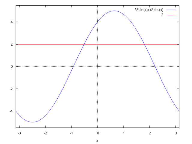
maxima
(%i1) load("trigtools")$
(%i2) eq:3*sin(x)+4*cos(x)=2$
(%i3) eq1:c2sin(lhs(eq))=2;
4
(%o3) 5 sin(x + atan(-)) = 2
3
(%i4) solvetrigwarn:false$
(%i5) solve(eq1)[1]$ x1:rhs(%);
2 4
(%o6) asin(-) - atan(-)
5 3
(%i7) float(%), numer;
(%o7) - 0.5157783719341241
(%i8) eq2:c2cos(lhs(eq))=2;
3
(%o8) 5 cos(x - atan(-)) = 2
4
(%i9) solve(eq2,x)[1]$ x2:rhs(%);
3 2
(%o10) atan(-) + acos(-)
4 5
(%i11) float(%), numer;
(%o11) 1.802780589520693
(%i12) sol:[x1,x2];
2 4 3 2
(%o12) [asin(-) - atan(-), atan(-) + acos(-)]
5 3 4 5
Answ.: $x = x_1 + 2\pi k,$ $x_1 = \sin^{-1}{2\over 5} - \tan^{-1}{4\over 3},$ or $x_1 = \tan^{-1}{3\over 4} + \cos^{-1}{2\over 5},$ for $k$ any integer.
c2trig (x) — Function
The function c2trig (convert to trigonometric) reduce expression with hyperbolic functions sinh, cosh, tanh, coth to trigonometric expression with sin, cos, tan, cot.
load("trigtools") loads these functions.
Examples:
maxima (%i1) load(trigtools)$
(%i2) sinh(x)=c2trig(sinh(x)); (%o2) sinh(x) = - %i sin(%i x)
(%i3) cosh(x)=c2trig(cosh(x)); (%o3) cosh(x) = cos(%i x)
(%i4) tanh(x)=c2trig(tanh(x)); (%o4) tanh(x) = - %i tan(%i x)
(%i5) coth(x)=c2trig(coth(x)); (%o5) coth(x) = %i cot(%i x)
2. see [https://maxima.sourceforge.io/ext/list_archives/2013/msg03230.html]()
```maxima
maxima
(%i1) load("trigtools")$
(%i2) cos(p+q*%i);
(%o2) cos(%i q + p)
(%i3) trigexpand(%);
(%o3) cos(p) cosh(q) - %i sin(p) sinh(q)
(%i4) c2trig(%);
(%o4) cos(%i q + p)
maxima (%i1) load(“trigtools”)$
(%i2) sin(a+b*%i); (%o2) sin(%i b + a)
(%i3) trigexpand(%); (%o3) %i cos(a) sinh(b) + sin(a) cosh(b)
(%i4) c2trig(%); (%o4) sin(%i b + a)
4. ```maxima
maxima
(%i1) load("trigtools")$
(%i2) cos(a*%i+b*%i);
(%o2) cos(%i b + %i a)
(%i3) trigexpand(%);
(%o3) sinh(a) sinh(b) + cosh(a) cosh(b)
(%i4) c2trig(%);
(%o4) cos(%i b + %i a)
maxima (%i1) load(“trigtools”)$
(%i2) tan(a+%i*b); (%o2) tan(%i b + a)
(%i3) trigexpand(%); %i tanh(b) + tan(a) (%o3) ——————— 1 - %i tan(a) tanh(b)
(%i4) c2trig(%); (%o4) tan(%i b + a)
6. ```maxima
maxima
(%i1) load("trigtools")$
(%i2) cot(x+%i*y);
(%o2) cot(%i y + x)
(%i3) trigexpand(%);
- %i cot(x) coth(y) - 1
(%o3) -----------------------
cot(x) - %i coth(y)
(%i4) c2trig(%);
(%o4) cot(%i y + x)
trigeval (x) — Function
The function trigeval compute values of expressions with $\sin {m\pi\over n},$ $\cos {m\pi\over n},$ $\tan {m\pi\over n},$ and $\cot {m\pi\over n}$ in radicals.
trigfactor (x) — Function
The function trigfactor factors expressions of form $\pm \sin x \pm \cos y.$
load("trigtools") loads this function.
Examples:
maxima (%i1) load(“trigtools”)$
(%i2) trigfactor(sin(x)+cos(x)); %pi (%o2) sqrt(2) cos(x - —) 4
(%i3) trigrat(%); (%o3) sin(x) + cos(x)
2. ```maxima
maxima
(%i1) load("trigtools")$
(%i2) trigfactor(sin(x)+cos(y));
y x %pi y x %pi
(%o2) 2 cos(- - - + ---) cos(- + - - ---)
2 2 4 2 2 4
(%i3) trigrat(%);
(%o3) cos(y) + sin(x)
maxima (%i1) load(“trigtools”)$
(%i2) trigfactor(sin(x)-cos(3*y)); 3 y x %pi 3 y x %pi (%o2) 2 sin(— - - + —) sin(— + - - —) 2 2 4 2 2 4
(%i3) trigrat(%); (%o3) sin(x) - cos(3 y)
4. ```maxima
maxima
(%i1) load("trigtools")$
(%i2) trigfactor(-sin(5*x)-cos(3*y));
3 y 5 x %pi 3 y 5 x %pi
(%o2) - 2 cos(--- - --- + ---) cos(--- + --- - ---)
2 2 4 2 2 4
(%i3) trigrat(%);
(%o3) - cos(3 y) - sin(5 x)
maxima (%i1) load(“trigtools”)$
(%i2) sin(alpha)+sin(beta)=trigfactor(sin(alpha)+sin(beta)); beta alpha (%o2) sin(beta) + sin(alpha) = 2 cos(–– - —–) 2 2 beta alpha sin(–– + —–) 2 2
(%i3) trigrat(%); (%o3) sin(beta) + sin(alpha) = sin(beta) + sin(alpha)
6. ```maxima
maxima
(%i1) load("trigtools")$
(%i2) sin(alpha)-sin(beta)=trigfactor(sin(alpha)-sin(beta));
beta alpha
(%o2) sin(alpha) - sin(beta) = - 2 sin(---- - -----)
2 2
beta alpha
cos(---- + -----)
2 2
maxima (%i1) load(“trigtools”)$
(%i2) cos(alpha)+cos(beta)=trigfactor(cos(alpha)+cos(beta)); beta alpha (%o2) cos(beta) + cos(alpha) = 2 cos(–– - —–) 2 2 beta alpha cos(–– + —–) 2 2
8. ```maxima
maxima
(%i1) load("trigtools")$
(%i2) cos(alpha)-cos(beta)=trigfactor(cos(alpha)-cos(beta));
beta alpha
(%o2) cos(alpha) - cos(beta) = 2 sin(---- - -----)
2 2
beta alpha
sin(---- + -----)
2 2
maxima (%i1) load(“trigtools”)$
(%i2) trigfactor(3sin(x)+7cos(x)); (%o2) 3 sin(x) + 7 cos(x)
(%i3) c2sin(%); 7 (%o3) sqrt(58) sin(x + atan(-)) 3
(%i4) trigexpand(%),expand; (%o4) 3 sin(x) + 7 cos(x)
10. ```maxima
maxima
(%i1) load("trigtools")$
(%i2) trigfactor(sin(2*x));
(%o2) sin(2 x)
(%i3) trigexpand(%);
(%o3) 2 cos(x) sin(x)
trigsolve (x) — Function
The function trigsolve find solutions of trigonometric equation from interval $[a,b).$
load("trigtools") loads this function.
Examples:
maxima
(%i1) eq:eq:3sin(x)+4cos(x)=2; (%o1) 3 sin(x) + 4 cos(x) = 2
(%i2) plot2d([3sin(x)+4cos(x),2],[x,-%pi,%pi]); (%o2) false

```maxima
maxima
(%i1) load("trigtools")$
(%i2) eq:eq:3*sin(x)+4*cos(x)=2$
(%i3) sol:trigsolve(eq,-%pi,%pi);
2 sqrt(21) 12 2 sqrt(21) 12
(%o3) {atan(---------- - --), %pi - atan(---------- + --)}
5 5 5 5
(%i4) float(%), numer;
(%o4) {- 0.5157783719341241, 1.8027805895206928}
Answ. : $x = \tan^{-1}\left({2\sqrt{21}\over 5} - {12\over 5}\right) + 2\pi k$ ; $x = \pi - \tan^{-1}\left({2\sqrt{21}\over 5} + {12\over 5}\right) + 2\pi k,$ $k$ – any integer. 2. ```maxima maxima (%i1) load(“trigtools”)$
(%i2) eq:cos(3x)-sin(x)=sqrt(3)(cos(x)-sin(3*x)); (%o2) cos(3 x) - sin(x) = sqrt(3) (cos(x) - sin(3 x))
(%i3) plot2d([lhs(eq)-rhs(eq)], [x,0,2*%pi])$
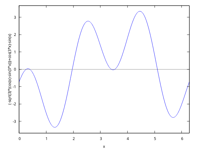
We have 6 solutions from [0, 2*pi].
```maxima
maxima
(%i1) load("trigtools")$
(%i2) eq:cos(3*x)-sin(x)=sqrt(3)*(cos(x)-sin(3*x))$
(%i3) plot2d([lhs(eq)-rhs(eq)], [x,0.2,0.5])$
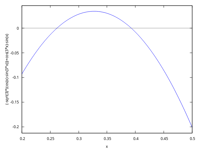
maxima
(%i1) load("trigtools")$
(%i2) load("trigtools")$
(%i3) eq:cos(3*x)-sin(x)=sqrt(3)*(cos(x)-sin(3*x))$
(%i4) plot2d([lhs(eq)-rhs(eq)], [x,3.3,3.6])$
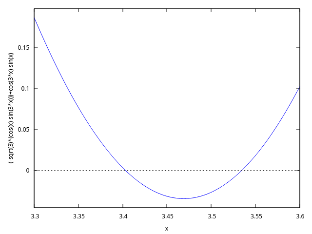
maxima
(%i1) load("trigtools")$
(%i2) eq:cos(3*x)-sin(x)=sqrt(3)*(cos(x)-sin(3*x))$
(%i3) trigfactor(lhs(eq))=map(trigfactor,rhs(eq));
%pi %pi
(%o3) - 2 sin(x + ---) sin(2 x - ---) =
4 4
%pi %pi
2 sqrt(3) sin(x - ---) sin(2 x - ---)
4 4
(%i4) factor(lhs(%)-rhs(%));
4 x + %pi 4 x - %pi
(%o4) - 2 (sin(---------) + sqrt(3) sin(---------))
4 4
8 x - %pi
sin(---------)
4
Equation is equivalent to
maxima
(%i1) load("trigtools")$
(%i2) eq:cos(3*x)-sin(x)=sqrt(3)*(cos(x)-sin(3*x))$
(%i3) trigfactor(lhs(eq))=map(trigfactor,rhs(eq));
%pi %pi
(%o3) - 2 sin(x + ---) sin(2 x - ---) =
4 4
%pi %pi
2 sqrt(3) sin(x - ---) sin(2 x - ---)
4 4
(%i4) L:factor(rhs(%)-lhs(%));
4 x + %pi 4 x - %pi 8 x - %pi
(%o4) 2 (sin(---------) + sqrt(3) sin(---------)) sin(---------)
4 4 4
(%i5) eq1:part(L,2)=0;
4 x + %pi 4 x - %pi
(%o5) sin(---------) + sqrt(3) sin(---------) = 0
4 4
(%i6) eq2:part(L,3)=0;
8 x - %pi
(%o6) sin(---------) = 0
4
(%i7) S1:trigsolve(eq1,0,2*%pi);
%pi 13 %pi
(%o7) {---, ------}
12 12
(%i8) S2:trigsolve(eq2,0,2*%pi);
%pi 5 %pi 9 %pi 13 %pi
(%o8) {---, -----, -----, ------}
8 8 8 8
(%i9) S:listify(union(S1,S2));
%pi %pi 5 %pi 13 %pi 9 %pi 13 %pi
(%o9) [---, ---, -----, ------, -----, ------]
12 8 8 12 8 8
(%i10) float(%), numer;
(%o10) [0.2617993877991494, 0.39269908169872414,
1.9634954084936207, 3.4033920413889422, 3.5342917352885173,
5.105088062083414]
Answer: $x = a + 2\pi k,$ where $a$ any from $S$, $k$ any integer. 3. ```maxima maxima (%i1) load(“trigtools”)$
(%i2) eq:8*cos(x)cos(4x)cos(5x)-1=0; (%o2) 8 cos(x) cos(4 x) cos(5 x) - 1 = 0
(%i3) trigrat(%); (%o3) 2 cos(10 x) + 2 cos(8 x) + 2 cos(2 x) + 1 = 0
Left side is periodic with period
$T=\pi.$
We have 10 solutions from [0, pi].
```maxima
maxima
(%i1) load("trigtools")$
(%i2) eq:8*cos(x)*cos(4*x)*cos(5*x)-1=0$
(%i3) plot2d([lhs(eq),rhs(eq)],[x,0,%pi]);
(%o3) false
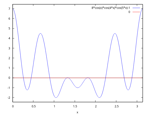
maxima
(%i1) load("trigtools")$
(%i2) eq:8*cos(x)*cos(4*x)*cos(5*x)-1=0$
(%i3) x4:find_root(eq, x, 1.3, 1.32);
(%o3) 1.3089969389957472
(%i4) x5:find_root(eq, x, 1.32, 1.35);
(%o4) 1.3463968515384828
(%i5) plot2d([lhs(eq),0], [x,1.3,1.35], [gnuplot_preamble, "set grid;"]);
(%o5) false
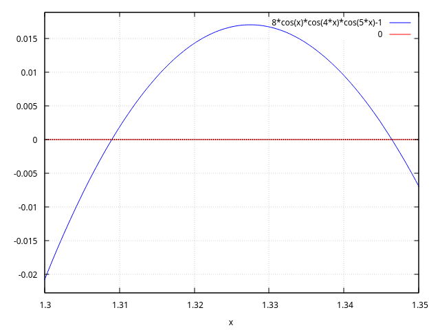
Equation we multiply by $2\sin x\cos 2x:$
maxima
(%i1) load("trigtools")$
(%i2) eq:8*cos(x)*cos(4*x)*cos(5*x)-1=0$
(%i3) eq*2*sin(x)*cos(2*x);
(%o3) 2 sin(x) cos(2 x) (8 cos(x) cos(4 x) cos(5 x) - 1) = 0
(%i4) eq1:trigreduce(%),expand;
(%o4) sin(13 x) + sin(x) = 0
(%i5) trigfactor(lhs(eq1))=0;
(%o5) 2 cos(6 x) sin(7 x) = 0
(%i6) S1:trigsolve(cos(6*x),0,%pi);
%pi %pi 5 %pi 7 %pi 3 %pi 11 %pi
(%o6) {---, ---, -----, -----, -----, ------}
12 4 12 12 4 12
(%i7) S2:trigsolve(sin(7*x),0,%pi);
%pi 2 %pi 3 %pi 4 %pi 5 %pi 6 %pi
(%o7) {0, ---, -----, -----, -----, -----, -----}
7 7 7 7 7 7
We remove solutions of $\sin x = 0$ and $\cos 2x = 0.$
maxima
(%i1) load("trigtools")$
(%i2) S1:trigsolve(cos(6*x),0,%pi)$
(%i3) S2:trigsolve(sin(7*x),0,%pi)$
(%i4) S3:trigsolve(sin(x),0,%pi);
(%o4) {0}
(%i5) S4:trigsolve(cos(2*x),0,%pi);
%pi 3 %pi
(%o5) {---, -----}
4 4
We find 10 solutions from $[0, \pi]:$
maxima
(%i1) load("trigtools")$
(%i2) S1:trigsolve(cos(6*x),0,%pi)$
(%i3) S2:trigsolve(sin(7*x),0,%pi)$
(%i4) S3:trigsolve(sin(x),0,%pi)$
(%i5) S4:trigsolve(cos(2*x),0,%pi)$
(%i6) union(S1,S2)$ setdifference(%,S3)$ setdifference(%,S4);
%pi %pi 2 %pi 5 %pi 3 %pi 4 %pi 7 %pi 5 %pi
(%o8) {---, ---, -----, -----, -----, -----, -----, -----,
12 7 7 12 7 7 12 7
6 %pi 11 %pi
-----, ------}
7 12
(%i9) S:listify(%);
%pi %pi 2 %pi 5 %pi 3 %pi 4 %pi 7 %pi 5 %pi
(%o9) [---, ---, -----, -----, -----, -----, -----, -----,
12 7 7 12 7 7 12 7
6 %pi 11 %pi
-----, ------]
7 12
(%i10) length(S);
(%o10) 10
(%i11) float(S), numer;
(%o11) [0.2617993877991494, 0.4487989505128276,
0.8975979010256552, 1.3089969389957472, 1.3463968515384828,
1.7951958020513104, 1.8325957145940461, 2.243994752564138,
2.6927937030769655, 2.8797932657906435]
Answer: $x = a + 2\pi k,$ where $a$ any from $S$, $k$ any integer.
trigvalue (x) — Function
The function trigvalue compute values of $\sin {m\pi\over n},$ $\cos {m\pi\over n},$ $\tan {m\pi\over n},$ and $\cot {m\pi\over n}$ in radicals.
trigvalue is essentially an internal function.
Use function trigeval in preference.
load("trigtools") loads this function.
See also: trigeval.
Units
ezunits
Function: `
The dimensional quantity operator.
An expression $a b$ represents a dimensional quantity, withaindicating a nondimensional quantity andbindicating the dimensional units. A symbol can be used as a unit without declaring it as such; unit symbols need not have any special properties. The quantity and unit of an expression $a b$ can
be extracted by the qty and units functions, respectively.
Arithmetic operations on dimensional quantities are carried out by conventional rules for such operations.
$(x a) * (y b)$ is equal to $(x * y) ` (a * b)$.
$(x a) + (y a)$ is equal to $(x + y) ` a$.
$(x a)^y$ is equal to $x^y a^y$ when y is nondimensional.
ezunits does not require that units in a sum have the same dimensions;
such terms are not added together, and no error is reported.
load ("ezunits") enables this operator.
Examples:
SI (Systeme Internationale) units.
(%i1) load ("ezunits")$
(%i2) foo : 10 ` m;
(%o2) 10 ` m
(%i3) qty (foo);
(%o3) 10
(%i4) units (foo);
(%o4) m
(%i5) dimensions (foo);
(%o5) length
“Customary” units.
(%i1) load ("ezunits")$
(%i2) bar : x ` acre;
(%o2) x ` acre
(%i3) dimensions (bar);
2
(%o3) length
(%i4) fundamental_units (bar);
2
(%o4) m
Units ad hoc.
(%i1) load ("ezunits")$
(%i2) baz : 3 ` sheep + 8 ` goat + 1 ` horse;
(%o2) 8 ` goat + 3 ` sheep + 1 ` horse
(%i3) subst ([sheep = 3*goat, horse = 10*goat], baz);
(%o3) 27 ` goat
(%i4) baz2 : 1000`gallon/fortnight;
gallon
(%o4) 1000 ` ---------
fortnight
(%i5) subst (fortnight = 14*day, baz2);
500 gallon
(%o5) --- ` ------
7 day
Arithmetic operations on dimensional quantities.
(%i1) load ("ezunits")$
(%i2) 100 ` kg + 200 ` kg;
(%o2) 300 ` kg
(%i3) 100 ` m^3 - 100 ` m^3;
3
(%o3) 0 ` m
(%i4) (10 ` kg) * (17 ` m/s^2);
kg m
(%o4) 170 ` ----
2
s
(%i5) (x ` m) / (y ` s);
x m
(%o5) - ` -
y s
(%i6) (a ` m)^2;
2 2
(%o6) a ` m
Function: ``
The unit conversion operator.
An expression $a b `` c$ converts from unitbto unitc. ezunitshas built-in conversions for SI base units, SI derived units, and some non-SI units. Unit conversions not already known toezunitscan be declared. The unit conversions known toezunitsare specified by the global variableknown_unit_conversions`,
which comprises built-in and user-defined conversions.
Conversions for products, quotients, and powers of units are
derived from the set of known unit conversions.
There is no preferred system for display of units;
input units are not converted to other units
unless conversion is explicitly indicated.
ezunits does not attempt to simplify units by prefixes
(milli-, centi-, deci-, etc)
unless such conversion is explicitly indicated.
load ("ezunits") enables this operator.
Examples:
The set of known unit conversions.
(%i1) load ("ezunits")$
(%i2) display2d : false$
(%i3) known_unit_conversions;
(%o3) {acre = 4840*yard^2,Btu = 1055*J,cfm = feet^3/minute,
cm = m/100,day = 86400*s,feet = 381*m/1250,ft = feet,
g = kg/1000,gallon = 757*l/200,GHz = 1000000000*Hz,
GOhm = 1000000000*Ohm,GPa = 1000000000*Pa,
GWb = 1000000000*Wb,Gg = 1000000*kg,Gm = 1000000000*m,
Gmol = 1000000*mol,Gs = 1000000000*s,ha = hectare,
hectare = 100*m^2,hour = 3600*s,Hz = 1/s,inch = feet/12,
km = 1000*m,kmol = 1000*mol,ks = 1000*s,l = liter,
lbf = pound_force,lbm = pound_mass,liter = m^3/1000,
metric_ton = Mg,mg = kg/1000000,MHz = 1000000*Hz,
microgram = kg/1000000000,micrometer = m/1000000,
micron = micrometer,microsecond = s/1000000,
mile = 5280*feet,minute = 60*s,mm = m/1000,
mmol = mol/1000,month = 2629800*s,MOhm = 1000000*Ohm,
MPa = 1000000*Pa,ms = s/1000,MWb = 1000000*Wb,
Mg = 1000*kg,Mm = 1000000*m,Mmol = 1000000000*mol,
Ms = 1000000*s,ns = s/1000000000,ounce = pound_mass/16,
oz = ounce,Ohm = s*J/C^2,
pound_force = 32*ft*pound_mass/s^2,
pound_mass = 200*kg/441,psi = pound_force/inch^2,
Pa = N/m^2,week = 604800*s,Wb = J/A,yard = 3*feet,
year = 31557600*s,C = s*A,F = C^2/J,GA = 1000000000*A,
GC = 1000000000*C,GF = 1000000000*F,GH = 1000000000*H,
GJ = 1000000000*J,GK = 1000000000*K,GN = 1000000000*N,
GS = 1000000000*S,GT = 1000000000*T,GV = 1000000000*V,
GW = 1000000000*W,H = J/A^2,J = m*N,kA = 1000*A,
kC = 1000*C,kF = 1000*F,kH = 1000*H,kHz = 1000*Hz,
kJ = 1000*J,kK = 1000*K,kN = 1000*N,kOhm = 1000*Ohm,
kPa = 1000*Pa,kS = 1000*S,kT = 1000*T,kV = 1000*V,
kW = 1000*W,kWb = 1000*Wb,mA = A/1000,mC = C/1000,
mF = F/1000,mH = H/1000,mHz = Hz/1000,mJ = J/1000,
mK = K/1000,mN = N/1000,mOhm = Ohm/1000,mPa = Pa/1000,
mS = S/1000,mT = T/1000,mV = V/1000,mW = W/1000,
mWb = Wb/1000,MA = 1000000*A,MC = 1000000*C,
MF = 1000000*F,MH = 1000000*H,MJ = 1000000*J,
MK = 1000000*K,MN = 1000000*N,MS = 1000000*S,
MT = 1000000*T,MV = 1000000*V,MW = 1000000*W,
N = kg*m/s^2,R = 5*K/9,S = 1/Ohm,T = J/(m^2*A),V = J/C,
W = J/s}
Elementary unit conversions.
(%i1) load ("ezunits")$
(%i2) 1 ` ft `` m;
Computing conversions to base units; may take a moment.
381
(%o2) ---- ` m
1250
(%i3) %, numer;
(%o3) 0.3048 ` m
(%i4) 1 ` kg `` lbm;
441
(%o4) --- ` lbm
200
(%i5) %, numer;
(%o5) 2.205 ` lbm
(%i6) 1 ` W `` Btu/hour;
720 Btu
(%o6) --- ` ----
211 hour
(%i7) %, numer;
Btu
(%o7) 3.412322274881517 ` ----
hour
(%i8) 100 ` degC `` degF;
(%o8) 212 ` degF
(%i9) -40 ` degF `` degC;
(%o9) (- 40) ` degC
(%i10) 1 ` acre*ft `` m^3;
60228605349 3
(%o10) ----------- ` m
48828125
(%i11) %, numer;
3
(%o11) 1233.48183754752 ` m
Coercing quantities in feet and meters to one or the other.
(%i1) load ("ezunits")$
(%i2) 100 ` m + 100 ` ft;
(%o2) 100 ` m + 100 ` ft
(%i3) (100 ` m + 100 ` ft) `` ft;
Computing conversions to base units; may take a moment.
163100
(%o3) ------ ` ft
381
(%i4) %, numer;
(%o4) 428.0839895013123 ` ft
(%i5) (100 ` m + 100 ` ft) `` m;
3262
(%o5) ---- ` m
25
(%i6) %, numer;
(%o6) 130.48 ` m
Dimensional analysis to find fundamental dimensions and fundamental units.
(%i1) load ("ezunits")$
(%i2) foo : 1 ` acre * ft;
(%o2) 1 ` acre ft
(%i3) dimensions (foo);
3
(%o3) length
(%i4) fundamental_units (foo);
3
(%o4) m
(%i5) foo `` m^3;
Computing conversions to base units; may take a moment.
60228605349 3
(%o5) ----------- ` m
48828125
(%i6) %, numer;
3
(%o6) 1233.48183754752 ` m
Declared unit conversions.
(%i1) load ("ezunits")$
(%i2) declare_unit_conversion (MMBtu = 10^6*Btu, kW = 1000*W);
(%o2) done
(%i3) declare_unit_conversion (kWh = kW*hour, MWh = 1000*kWh,
bell = 1800*s);
(%o3) done
(%i4) 1 ` kW*s `` MWh;
Computing conversions to base units; may take a moment.
1
(%o4) ------- ` MWh
3600000
(%i5) 1 ` kW/m^2 `` MMBtu/bell/ft^2;
1306449 MMBtu
(%o5) ---------- ` --------
8242187500 2
bell ft
constvalue (x) — Function
Shows the value and the units of one of the constants declared by package
physical_constants, which includes a list of physical constants, or
of a new constant declared in package ezunits (see
declare_constvalue).
Note that constant values as recognized by constvalue
are separate from values declared by numerval and
recognized by constantp.
Example:
(%i1) load ("physical_constants")$
(%i2) constvalue (%G);
3
m
(%o2) 6.67428 ` -----
2
kg s
(%i3) get ('%G, 'description);
(%o3) Newtonian constant of gravitation
See also: declare_constvalue.
declare_constvalue (a, x) — Function
Declares the value of a constant to be used in package ezunits. This
function should be loaded with load ("ezunits").
Example:
(%i1) load ("ezunits")$
(%i2) declare_constvalue (FOO, 100 ` lbm / acre);
lbm
(%o2) 100 ` ----
acre
(%i3) FOO * (50 ` acre);
(%o3) 50 FOO ` acre
(%i4) constvalue (%);
(%o4) 5000 ` lbm
declare_dimensions (a_1, d_1, …, a_n, d_n) — Function
Declares a_1, …, a_n to have dimensions d_1, …, d_n, respectively.
Each a_k is a symbol or a list of symbols. If it is a list, then every symbol in a_k is declared to have dimension d_k.
load ("ezunits") loads these functions.
Examples:
(%i1) load ("ezunits") $
(%i2) declare_dimensions ([x, y, z], length, [t, u], time);
(%o2) done
(%i3) dimensions (y^2/u);
2
length
(%o3) -------
time
(%i4) fundamental_units (y^2/u);
0 errors, 0 warnings
2
m
(%o4) --
s
declare_fundamental_dimensions (d_1, d_2, d_3, …) — Function
declare_fundamental_dimensions declares fundamental dimensions.
Symbols d_1, d_2, d_3, … are appended to the list of
fundamental dimensions, if they are not already on the list.
remove_fundamental_dimensions reverts the effect of declare_fundamental_dimensions.
fundamental_dimensions is the list of fundamental dimensions.
By default, the list comprises several physical dimensions.
load ("ezunits") loads these functions.
Examples:
(%i1) load ("ezunits") $
(%i2) fundamental_dimensions;
(%o2) [length, mass, time, current, temperature, quantity]
(%i3) declare_fundamental_dimensions (money, cattle, happiness);
(%o3) done
(%i4) fundamental_dimensions;
(%o4) [length, mass, time, current, temperature, quantity,
money, cattle, happiness]
(%i5) remove_fundamental_dimensions (cattle, happiness);
(%o5) done
(%i6) fundamental_dimensions;
(%o6) [length, mass, time, current, temperature, quantity, money]
declare_fundamental_units (u_1, d_1, …, u_n, d_n) — Function
declare_fundamental_units declares u_1, …, u_n
to have dimensions d_1, …, d_n, respectively.
All arguments must be symbols.
After calling declare_fundamental_units,
dimensions(u_k) returns d_k for each argument u_1, …, u_n,
and fundamental_units(d_k) returns u_k for each argument d_1, …, d_n.
remove_fundamental_units reverts the effect of declare_fundamental_units.
load ("ezunits") loads these functions.
Examples:
(%i1) load ("ezunits") $
(%i2) declare_fundamental_dimensions (money, cattle, happiness);
(%o2) done
(%i3) declare_fundamental_units (dollar, money, goat, cattle,
smile, happiness);
(%o3) [dollar, goat, smile]
(%i4) dimensions (100 ` dollar/goat/km^2);
money
(%o4) --------------
2
cattle length
(%i5) dimensions (x ` smile/kg);
happiness
(%o5) ---------
mass
(%i6) fundamental_units (money*cattle/happiness);
0 errors, 0 warnings
dollar goat
(%o6) -----------
smile
declare_qty (a, x) — Function
Declares that qty should return x for symbol a, where
x is a nondimensional quantity. This function should be loaded
with load ("ezunits").
Example:
(%i1) load ("ezunits")$
(%i2) declare_qty (aa, xx);
(%o2) xx
(%i3) qty (aa);
(%o3) xx
(%i4) qty (aa^2);
2
(%o4) xx
(%i5) foo : 100 ` kg;
(%o5) 100 ` kg
(%i6) qty (aa * foo);
(%o6) 100 xx
See also: qty.
declare_unit_conversion (u=v, …) — Function
Appends equations u = v, … to the list of unit conversions known to the unit conversion operator $``$. u and v are both multiplicative terms, in which any variables are units, or both literal dimensional expressions.
At present, it is necessary to express conversions such that the left-hand side of each equation is a simple unit (not a multiplicative expression) or a literal dimensional expression with the quantity equal to 1 and the unit being a simple unit. This limitation might be relaxed in future versions.
known_unit_conversions is the list of known unit conversions.
This function should be loaded with load ("ezunits").
Examples:
Unit conversions expressed by equations of multiplicative terms.
(%i1) load ("ezunits")$
(%i2) declare_unit_conversion (nautical_mile = 1852 * m,
fortnight = 14 * day);
(%o2) done
(%i3) 100 ` nautical_mile / fortnight `` m/s;
Computing conversions to base units; may take a moment.
463 m
(%o3) ---- ` -
3024 s
Unit conversions expressed by equations of literal dimensional expressions.
(%i1) load ("ezunits")$
(%i2) declare_unit_conversion (1 ` fluid_ounce = 2 ` tablespoon);
(%o2) done
(%i3) declare_unit_conversion (1 ` tablespoon = 3 ` teaspoon);
(%o3) done
(%i4) 15 ` fluid_ounce `` teaspoon;
Computing conversions to base units; may take a moment.
(%o4) 90 ` teaspoon
declare_units (a, u) — Function
Declares that units should return units u for a,
where u is an expression. This function should be loaded with
load ("ezunits").
Example:
(%i1) load ("ezunits")$
(%i2) units (aa);
(%o2) 1
(%i3) declare_units (aa, J);
(%o3) J
(%i4) units (aa);
(%o4) J
(%i5) units (aa^2);
2
(%o5) J
(%i6) foo : 100 ` kg;
(%o6) 100 ` kg
(%i7) units (aa * foo);
(%o7) kg J
See also: units.
dimensionless (L) — Function
Returns a basis for the dimensionless quantities which can be formed from a list L of dimensional quantities.
load ("ezunits") loads this function.
Examples:
(%i1) load ("ezunits") $
(%i2) dimensionless ([x ` m, y ` m/s, z ` s]);
0 errors, 0 warnings
0 errors, 0 warnings
y z
(%o2) [---]
x
Dimensionless quantities derived from fundamental physical quantities. Note that the first element on the list is proportional to the fine-structure constant.
(%i1) load ("ezunits") $
(%i2) load ("physical_constants") $
(%i3) dimensionless([%h_bar, %m_e, %m_P, %%e, %c, %e_0]);
0 errors, 0 warnings
0 errors, 0 warnings
2
%%e %m_e
(%o3) [--------------, ----]
%c %e_0 %h_bar %m_P
fundamental_units (x) — Function
fundamental_units(x) returns the units
associated with the fundamental dimensions of x.
as determined by dimensions(x).
x may be a literal dimensional expression $a b$, a symbol with declared units viadeclare_units`,
or an expression containing either or both of those.
fundamental_units() returns the list of all known fundamental units,
as declared by declare_fundamental_units.
load ("ezunits") loads this function.
Examples:
(%i1) load ("ezunits")$
(%i2) fundamental_units ();
(%o2) [m, kg, s, A, K, mol]
(%i3) fundamental_units (100 ` mile/hour);
m
(%o3) -
s
(%i4) declare_units (aa, g/foot^2);
g
(%o4) -----
2
foot
(%i5) fundamental_units (aa);
kg
(%o5) --
2
m
natural_unit (expr, [v_1, …, v_n]) — Function
Finds exponents e_1, …, e_n such that
dimension(expr) = dimension(v_1^e_1 ... v_n^e_n).
load ("ezunits") loads this function.
Examples:
qty (x) — Function
Returns the nondimensional part of a dimensional quantity x, or returns x if x is nondimensional. x may be a literal dimensional expression $a ` b$, a symbol with declared quantity, or an expression containing either or both of those.
This function should be loaded with load ("ezunits").
Example:
(%i1) load ("ezunits")$
(%i2) foo : 100 ` kg;
(%o2) 100 ` kg
(%i3) qty (foo);
(%o3) 100
(%i4) bar : v ` m/s;
m
(%o4) v ` -
s
(%i5) foo * bar;
kg m
(%o5) 100 v ` ----
s
(%i6) qty (foo * bar);
(%o6) 100 v
remove_constvalue (a) — Function
Reverts the effect of declare_005fconstvalue. This function should be
loaded with load ("ezunits").
See also: declare_constvalue.
remove_dimensions (a_1, …, a_n) — Function
Reverts the effect of declare_dimensions. This function should be
loaded with load ("ezunits").
unitp (x) — Function
Returns true if x is a literal dimensional expression,
a symbol declared dimensional,
or an expression in which the main operator is declared dimensional.
unitp returns false otherwise.
load ("ezunits") loads this function.
Examples:
unitp applied to a literal dimensional expression.
(%i1) load ("ezunits")$
(%i2) unitp (100 ` kg);
(%o2) true
unitp applied to a symbol declared dimensional.
(%i1) load ("ezunits")$
(%i2) unitp (foo);
(%o2) false
(%i3) declare (foo, dimensional);
(%o3) done
(%i4) unitp (foo);
(%o4) true
unitp applied to an expression in which the main operator is declared dimensional.
(%i1) load ("ezunits")$
(%i2) unitp (bar (x, y, z));
(%o2) false
(%i3) declare (bar, dimensional);
(%o3) done
(%i4) unitp (bar (x, y, z));
(%o4) true
units (x) — Function
Returns the units of a dimensional quantity x, or returns 1 if x is nondimensional.
x may be a literal dimensional expression $a b$, a symbol with declared units viadeclare_units`,
or an expression containing either or both of those.
This function should be loaded with load ("ezunits").
Example:
(%i1) load ("ezunits")$
(%i2) foo : 100 ` kg;
(%o2) 100 ` kg
(%i3) bar : x ` m/s;
m
(%o3) x ` -
s
(%i4) units (foo);
(%o4) kg
(%i5) units (bar);
m
(%o5) -
s
(%i6) units (foo * bar);
kg m
(%o6) ----
s
(%i7) units (foo / bar);
kg s
(%o7) ----
m
(%i8) units (foo^2);
2
(%o8) kg
unit
%unitexpand — Variable
Default value: 2
This is the value supplied to metricexpandall during the initial loading
of unit.
convert (expr, list) — Function
When resetting the global environment is overkill, there is the convert
command, which allows one time conversions. It can accept either a single
argument or a list of units to use in conversion. When a convert operation is
done, the normal global evaluation system is bypassed, in order to avoid the
desired result being converted again. As a consequence, for inexact calculations
“rat” warnings will be visible if the global environment controlling this behavior
(ratprint) is true. This is also useful for spot-checking the
accuracy of a global conversion. Another feature is convert will allow a
user to do Base Dimension conversions even if the global environment is set to
simplify to a Derived Dimension.
(%i2) kg*m/s^2;
kg m
(%o2) ----
2
s
(%i3) convert(kg*m/s^2,[g,km,s]);
g km
(%o3) ----
2
s
(%i4) convert(kg*m/s^2,[g,inch,minute]);
`rat' replaced 39.37007874015748 by 5000/127 = 39.37007874015748
18000000000 %in g
(%o4) (-----------) (-----)
127 2
%min
(%i5) convert(kg*m/s^2,[N]);
(%o5) N
(%i6) convert(kg*m^2/s^2,[N]);
(%o6) m N
(%i7) setunits([N,J]);
(%o7) done
(%i8) convert(kg*m^2/s^2,[N]);
(%o8) m N
(%i9) convert(kg*m^2/s^2,[N,inch]);
`rat' replaced 39.37007874015748 by 5000/127 = 39.37007874015748
5000
(%o9) (----) (%in N)
127
(%i10) convert(kg*m^2/s^2,[J]);
(%o10) J
(%i11) kg*m^2/s^2;
(%o11) J
(%i12) setunits([g,inch,s]);
(%o12) done
(%i13) kg*m/s^2;
(%o13) N
(%i14) uforget(N);
(%o14) false
(%i15) kg*m/s^2;
5000000 %in g
(%o15) (-------) (-----)
127 2
s
(%i16) convert(kg*m/s^2,[g,inch,s]);
`rat' replaced 39.37007874015748 by 5000/127 = 39.37007874015748
5000000 %in g
(%o16) (-------) (-----)
127 2
s
See also setunits and uforget. To use this function write first load("unit").
See also: setunits, uforget.
metricexpandall (x) — Function
Rebuilds global unit lists automatically creating all desired metric units. x is a numerical argument which is used to specify how many metric prefixes the user wishes defined. The arguments are as follows, with each higher number defining all lower numbers’ units:
0 - none. Only base units
1 - kilo, centi, milli
(default) 2 - giga, mega, kilo, hecto, deka, deci, centi, milli,
micro, nano
3 - peta, tera, giga, mega, kilo, hecto, deka, deci,
centi, milli, micro, nano, pico, femto
4 - all
Normally, Maxima will not define the full expansion since this results in a
very large number of units, but metricexpandall can be used to
rebuild the list in a more or less complete fashion. The relevant variable
in the unit.mac file is %unitexpand.
setunits (list) — Function
By default, the unit package does not use any derived dimensions, but will convert all units to the seven fundamental dimensions using MKS units.
(%i2) N;
kg m
(%o2) ----
2
s
(%i3) dyn;
1 kg m
(%o3) (------) (----)
100000 2
s
(%i4) g;
1
(%o4) (----) (kg)
1000
(%i5) centigram*inch/minutes^2;
127 kg m
(%o5) (-------------) (----)
1800000000000 2
s
In some cases this is the desired behavior. If the user wishes to use other
units, this is achieved with the setunits command:
(%i6) setunits([centigram,inch,minute]);
(%o6) done
(%i7) N;
1800000000000 %in cg
(%o7) (-------------) (------)
127 2
%min
(%i8) dyn;
18000000 %in cg
(%o8) (--------) (------)
127 2
%min
(%i9) g;
(%o9) (100) (cg)
(%i10) centigram*inch/minutes^2;
%in cg
(%o10) ------
2
%min
The setting of units is quite flexible. For example, if we want to get back to kilograms, meters, and seconds as defaults for those dimensions we can do:
(%i11) setunits([kg,m,s]);
(%o11) done
(%i12) centigram*inch/minutes^2;
127 kg m
(%o12) (-------------) (----)
1800000000000 2
s
Derived units are also handled by this command:
(%i17) setunits(N);
(%o17) done
(%i18) N;
(%o18) N
(%i19) dyn;
1
(%o19) (------) (N)
100000
(%i20) kg*m/s^2;
(%o20) N
(%i21) centigram*inch/minutes^2;
127
(%o21) (-------------) (N)
1800000000000
Notice that the unit package recognized the non MKS combination of mass, length, and inverse time squared as a force, and converted it to Newtons. This is how Maxima works in general. If, for example, we prefer dyne to Newtons, we simply do the following:
(%i22) setunits(dyn);
(%o22) done
(%i23) kg*m/s^2;
(%o23) (100000) (dyn)
(%i24) centigram*inch/minutes^2;
127
(%o24) (--------) (dyn)
18000000
To discontinue simplifying to any force, we use the uforget command:
(%i26) uforget(dyn);
(%o26) false
(%i27) kg*m/s^2;
kg m
(%o27) ----
2
s
(%i28) centigram*inch/minutes^2;
127 kg m
(%o28) (-------------) (----)
1800000000000 2
s
This would have worked equally well with uforget(N) or
uforget(%force).
See also uforget. To use this function write first load("unit").
See also: uforget.
uforget (list) — Function
By default, the unit package converts all units to the
seven fundamental dimensions using MKS units. This behavior can
be changed with the setunits command. After that, the
user can restore the default behavior for a particular dimension
by means of the uforget command:
(%i13) setunits([centigram,inch,minute]);
(%o13) done
(%i14) centigram*inch/minutes^2;
%in cg
(%o14) ------
2
%min
(%i15) uforget([cg,%in,%min]);
(%o15) [false, false, false]
(%i16) centigram*inch/minutes^2;
127 kg m
(%o16) (-------------) (----)
1800000000000 2
s
uforget operates on dimensions,
not units, so any unit of a particular dimension will work. The
dimension itself is also a legal argument.
See also setunits. To use this function write first load("unit").
See also: setunits.
usersetunits — Variable
Default value: none
If a user wishes to have a default unit behavior other than that described,
they can make use of maxima-init.mac and the usersetunits
variable. The unit package will check on startup to see if this variable
has been assigned a list. If it has, it will use setunits on that list and take
the units from that list to be defaults. uforget will revert to the behavior
defined by usersetunits over its own defaults. For example, if we have a
maxima-init.mac file containing:
usersetunits : [N,J];
we would see the following behavior:
(%i1) load("unit")$
*******************************************************************
* Units version 0.50 *
* Definitions based on the NIST Reference on *
* Constants, Units, and Uncertainty *
* Conversion factors from various sources including *
* NIST and the GNU units package *
*******************************************************************
Redefining necessary functions...
WARNING: DEFUN/DEFMACRO: redefining function
TOPLEVEL-MACSYMA-EVAL ...
WARNING: DEFUN/DEFMACRO: redefining function MSETCHK ...
WARNING: DEFUN/DEFMACRO: redefining function KILL1 ...
WARNING: DEFUN/DEFMACRO: redefining function NFORMAT ...
Initializing unit arrays...
Done.
User defaults found...
User defaults initialized.
(%i2) kg*m/s^2;
(%o2) N
(%i3) kg*m^2/s^2;
(%o3) J
(%i4) kg*m^3/s^2;
(%o4) J m
(%i5) kg*m*km/s^2;
(%o5) (1000) (J)
(%i6) setunits([dyn,eV]);
(%o6) done
(%i7) kg*m/s^2;
(%o7) (100000) (dyn)
(%i8) kg*m^2/s^2;
(%o8) (6241509596477042688) (eV)
(%i9) kg*m^3/s^2;
(%o9) (6241509596477042688) (eV m)
(%i10) kg*m*km/s^2;
(%o10) (6241509596477042688000) (eV)
(%i11) uforget([dyn,eV]);
(%o11) [false, false]
(%i12) kg*m/s^2;
(%o12) N
(%i13) kg*m^2/s^2;
(%o13) J
(%i14) kg*m^3/s^2;
(%o14) J m
(%i15) kg*m*km/s^2;
(%o15) (1000) (J)
Without usersetunits, the initial inputs would have been converted
to MKS, and uforget would have resulted in a return to MKS rules. Instead,
the user preferences are respected in both cases. Notice these can still
be overridden if desired. To completely eliminate this simplification - i.e.
to have the user defaults reset to factory defaults - the dontusedimension
command can be used. uforget can restore user settings again, but
only if usedimension frees it for use. Alternately,
kill(usersetunits) will completely remove all knowledge of the user defaults
from the session. Here are some examples of how these various options work.
(%i2) kg*m/s^2;
(%o2) N
(%i3) kg*m^2/s^2;
(%o3) J
(%i4) setunits([dyn,eV]);
(%o4) done
(%i5) kg*m/s^2;
(%o5) (100000) (dyn)
(%i6) kg*m^2/s^2;
(%o6) (6241509596477042688) (eV)
(%i7) uforget([dyn,eV]);
(%o7) [false, false]
(%i8) kg*m/s^2;
(%o8) N
(%i9) kg*m^2/s^2;
(%o9) J
(%i10) dontusedimension(N);
(%o10) [%force]
(%i11) dontusedimension(J);
(%o11) [%energy, %force]
(%i12) kg*m/s^2;
kg m
(%o12) ----
2
s
(%i13) kg*m^2/s^2;
2
kg m
(%o13) -----
2
s
(%i14) setunits([dyn,eV]);
(%o14) done
(%i15) kg*m/s^2;
kg m
(%o15) ----
2
s
(%i16) kg*m^2/s^2;
2
kg m
(%o16) -----
2
s
(%i17) uforget([dyn,eV]);
(%o17) [false, false]
(%i18) kg*m/s^2;
kg m
(%o18) ----
2
s
(%i19) kg*m^2/s^2;
2
kg m
(%o19) -----
2
s
(%i20) usedimension(N);
Done. To have Maxima simplify to this dimension, use
setunits([unit]) to select a unit.
(%o20) true
(%i21) usedimension(J);
Done. To have Maxima simplify to this dimension, use
setunits([unit]) to select a unit.
(%o21) true
(%i22) kg*m/s^2;
kg m
(%o22) ----
2
s
(%i23) kg*m^2/s^2;
2
kg m
(%o23) -----
2
s
(%i24) setunits([dyn,eV]);
(%o24) done
(%i25) kg*m/s^2;
(%o25) (100000) (dyn)
(%i26) kg*m^2/s^2;
(%o26) (6241509596477042688) (eV)
(%i27) uforget([dyn,eV]);
(%o27) [false, false]
(%i28) kg*m/s^2;
(%o28) N
(%i29) kg*m^2/s^2;
(%o29) J
(%i30) kill(usersetunits);
(%o30) done
(%i31) uforget([dyn,eV]);
(%o31) [false, false]
(%i32) kg*m/s^2;
kg m
(%o32) ----
2
s
(%i33) kg*m^2/s^2;
2
kg m
(%o33) -----
2
s
Unfortunately this wide variety of options is a little confusing at first, but once the user grows used to them they should find they have very full control over their working environment.