draw
allocation — Variable
Default value: false
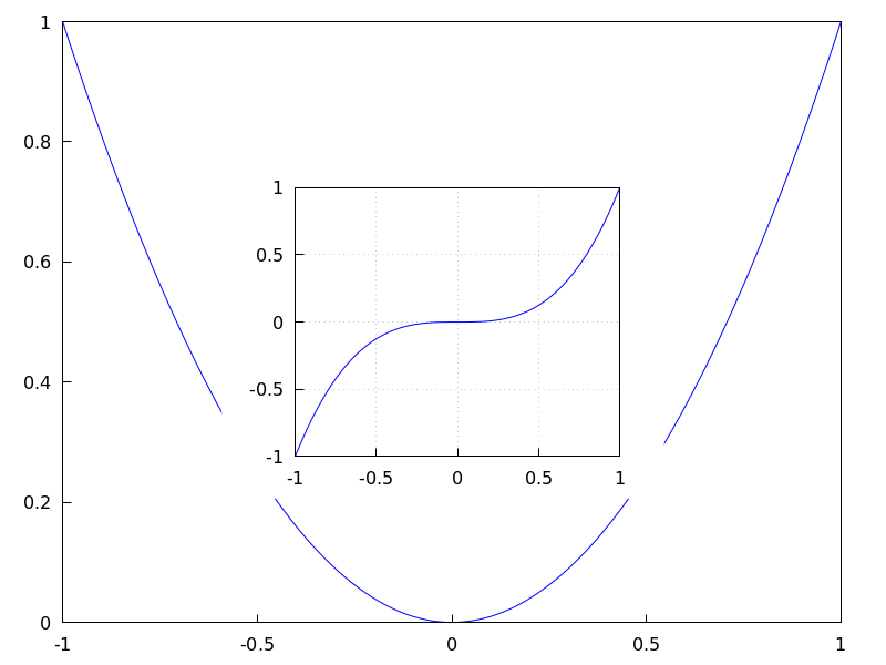
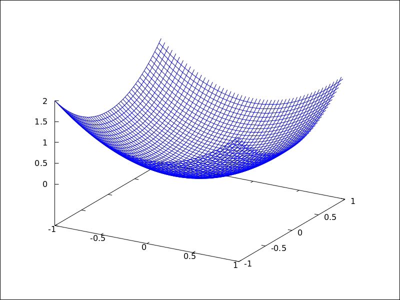
With option allocation it is possible to place a scene in the
output window at will; this is of interest in multiplots. When false,
the scene is placed automatically, depending on the value assigned to option
columns. In any other case, allocation must be set to a list of
two pairs of numbers; the first corresponds to the position of the lower left
corner of the scene, and the second pair gives the width and height of the plot.
All quantities must be given in relative coordinates, between 0 and 1.
Examples:
In site graphics.
(%i1) draw(
        gr2d(
          explicit(x^2,x,-1,1)),
        gr2d(
          allocation = [[1/4, 1/4],[1/2, 1/2]],
          explicit(x^3,x,-1,1),
          grid = true) ) $
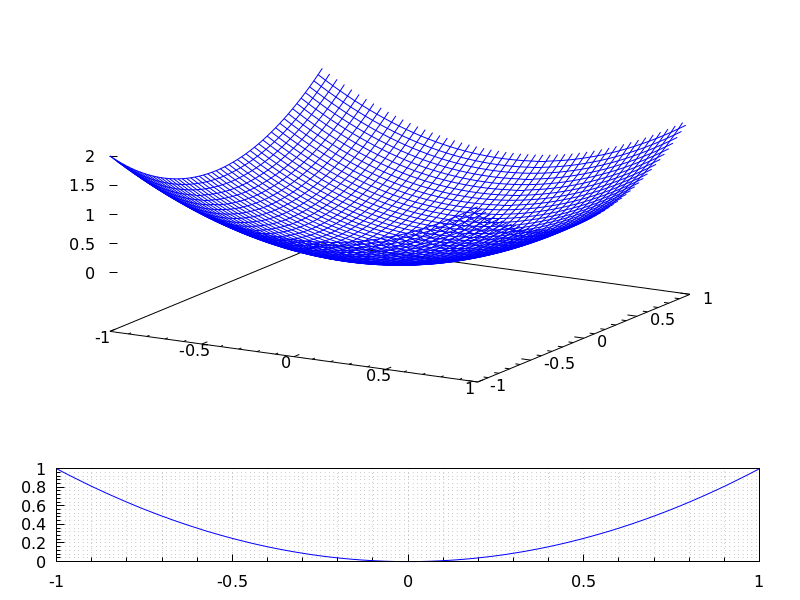
Multiplot with selected dimensions.
(%i1) draw(
        terminal = wxt,
        gr2d(
          grid=[5,5],
          allocation = [[0, 0],[1, 1/4]],
          explicit(x^2,x,-1,1)),
        gr3d(
          allocation = [[0, 1/4],[1, 3/4]],
          explicit(x^2+y^2,x,-1,1,y,-1,1) ))$
See also option columns.
See also: columns.
axis_3d — Variable
Default value: true
If axis_3d is true, the x, y and z axis are shown in 3d scenes.
Since this is a global graphics option, its position in the scene description does not matter.
Example:
(%i1) draw3d(axis_3d = false,
             explicit(sin(x^2+y^2),x,-2,2,y,-2,2) )$
See also axis_bottom, axis_left, axis_top, and axis_right for axis in 2d.
See also: axis_bottom, axis_left, axis_top, axis_right.
axis_bottom — Variable
Default value: true
If axis_bottom is true, the bottom axis is shown in 2d scenes.
Since this is a global graphics option, its position in the scene description does not matter.
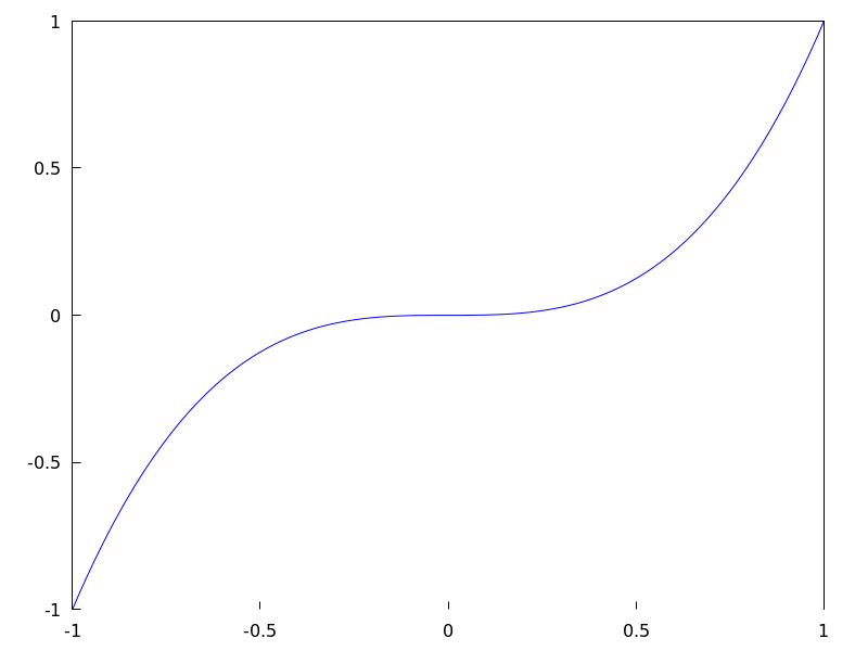
Example:
(%i1) draw2d(axis_bottom = false,
             explicit(x^3,x,-1,1))$
See also axis_left, axis_top, axis_right and axis_005f3d.
See also: axis_left, axis_top, axis_right, axis_3d.
axis_left — Variable
Default value: true
If axis_left is true, the left axis is shown in 2d scenes.
Since this is a global graphics option, its position in the scene description does not matter.
Example:
(%i1) draw2d(axis_left = false,
             explicit(x^3,x,-1,1))$
See also axis_bottom, axis_top, axis_right and axis_005f3d.
See also: axis_bottom, axis_top, axis_right, axis_3d.
axis_right — Variable
Default value: true
If axis_right is true, the right axis is shown in 2d scenes.
Since this is a global graphics option, its position in the scene description does not matter.
Example:
(%i1) draw2d(axis_right = false,
             explicit(x^3,x,-1,1))$
See also axis_bottom, axis_left, axis_top and axis_005f3d.
See also: axis_bottom, axis_left, axis_top, axis_3d.
axis_top — Variable
Default value: true
If axis_top is true, the top axis is shown in 2d scenes.
Since this is a global graphics option, its position in the scene description does not matter.
Example:
(%i1) draw2d(axis_top = false,
             explicit(x^3,x,-1,1))$
See also axis_bottom, axis_left, axis_right, and axis_005f3d.
See also: axis_bottom, axis_left, axis_right, axis_3d.
background_color — Variable
Default value: white
Sets the background color for terminals. Default background color is white.
Since this is a global graphics option, its position in the scene description does not matter.
This option does not work with terminals epslatex and epslatex_standalone.
See also color
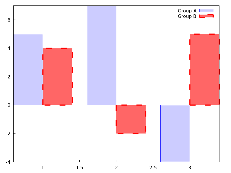
bars ([x1, h1, w1], [x2, h2, w2, …]) — Function
Draws vertical bars in 2D.
2D
bars ([x1,h1,w1], [x2,h2,w2, ...])
draws bars centered at values x1, x2, … with heights h1, h2, …
and widths w1, w2, …
This object is affected by the following graphic options: key,
fill_color, fill_density and line_005fwidth.
Example:
(%i1) draw2d(
       key          = "Group A",
       fill_color   = blue,
       fill_density = 0.2,
       bars([0.8,5,0.4],[1.8,7,0.4],[2.8,-4,0.4]),
       key          = "Group B",
       fill_color   = red,
       fill_density = 0.6,
       line_width   = 4,
       bars([1.2,4,0.4],[2.2,-2,0.4],[3.2,5,0.4]),
       xaxis = true);
See also: key, fill_color, fill_density, line_width.
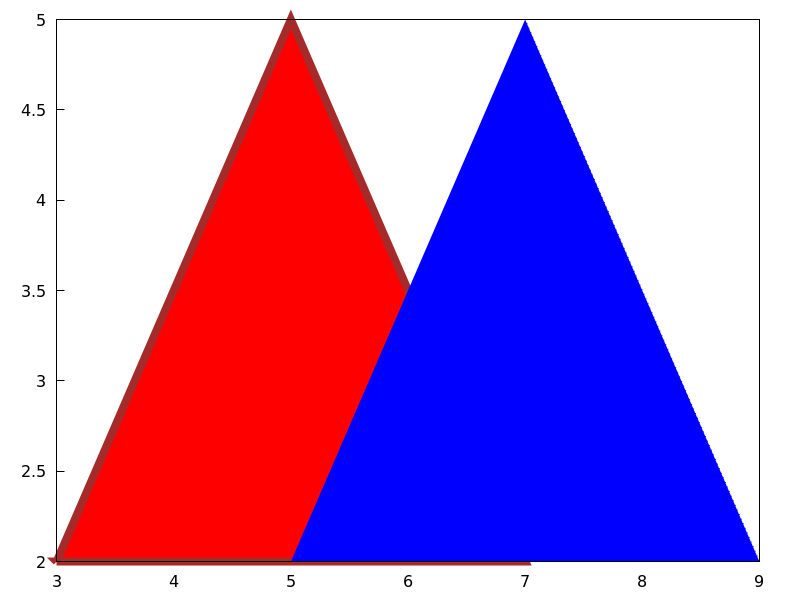
border — Variable
Default value: true
If border is true, borders of polygons are painted
according to line_type and line_width.
This option affects the following graphic objects:
gr2d: polygon, rectangle and ellipse.
Example:
(%i1) draw2d(color       = brown,
             line_width  = 8,
             polygon([[3,2],[7,2],[5,5]]),
             border      = false,
             fill_color  = blue,
             polygon([[5,2],[9,2],[7,5]]) )$
See also: polygon, rectangle, ellipse.
boundaries_array — Variable
Default value: false
boundaries_array is where the graphic object geomap looks
for boundaries coordinates.
Each component of boundaries_array is an array of floating
point quantities, the coordinates of a polygonal segment or map boundary.
See also geomap.
See also: geomap.
capping — Variable
Default value: [false, false]
A list with two possible elements, true and false,
indicating whether the extremes of a graphic object tube remain closed
or open. By default, both extremes are left open.
Setting capping = false is equivalent to capping = [false, false],
and capping = true is equivalent to capping = [true, true].
Example:
(%i1) draw3d(
        capping = [false, true],
        tube(0, 0, a, 1,
             a, 0, 8) )$
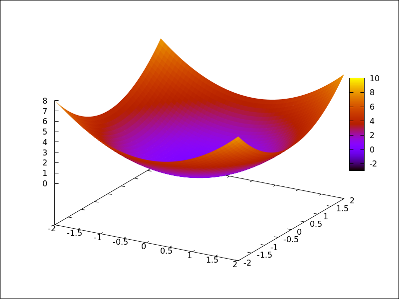
cbrange — Variable
Default value: auto
If cbrange is auto, the range for the values which are
colored when enhanced3d is not false is computed
automatically. Values outside of the color range use color of the
nearest extreme.
When enhanced3d or colorbox is false, option cbrange has
no effect.
If the user wants a specific interval for the colored values, it must
be given as a Maxima list, as in cbrange=[-2, 3].
Since this is a global graphics option, its position in the scene description does not matter.
Example:
(%i1) draw3d (
        enhanced3d     = true,
        color          = green,
        cbrange = [-3,10],
        explicit(x^2+y^2, x,-2,2,y,-2,2)) $
See also enhanced3d, colorbox and cbtics.
See also: enhanced3d, colorbox, cbtics.
cbtics — Variable
Default value: auto
This graphic option controls the way tic marks are drawn on the colorbox
when option enhanced3d is not false.
When enhanced3d or colorbox is false, option cbtics has
no effect.
See xtics for a complete description.
Example :
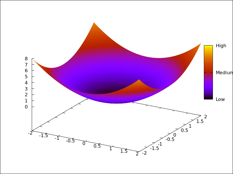
(%i1) draw3d (
        enhanced3d = true,
        color      = green,
        cbtics  = {["High",10],["Medium",05],["Low",0]},
        cbrange = [0, 10],
        explicit(x^2+y^2, x,-2,2,y,-2,2)) $
See also enhanced3d, colorbox and cbrange.
See also: enhanced3d, colorbox, cbrange.
colorbox — Variable
Default value: true
If colorbox is true, a color scale without label is drawn together with
image 2D objects, or coloured 3d objects. If colorbox is false, no
color scale is shown. If colorbox is a string, a color scale with label is drawn.
Since this is a global graphics option, its position in the scene description does not matter.
Example:
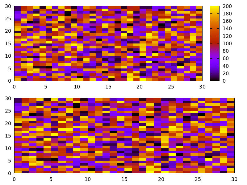
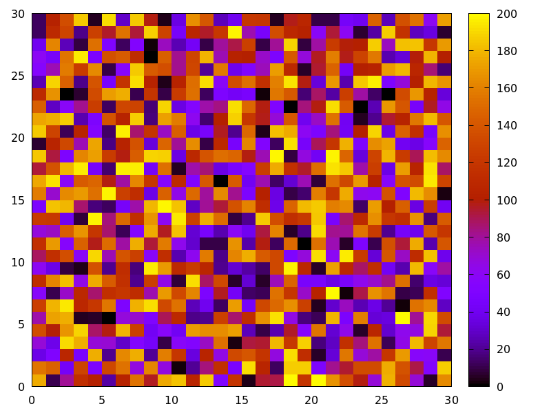
Color scale and images.
(%i1) im: apply('matrix,
                 makelist(makelist(random(200),i,1,30),i,1,30))$
(%i2) draw(
          gr2d(image(im,0,0,30,30)),
          gr2d(colorbox = false, image(im,0,0,30,30))
      )$
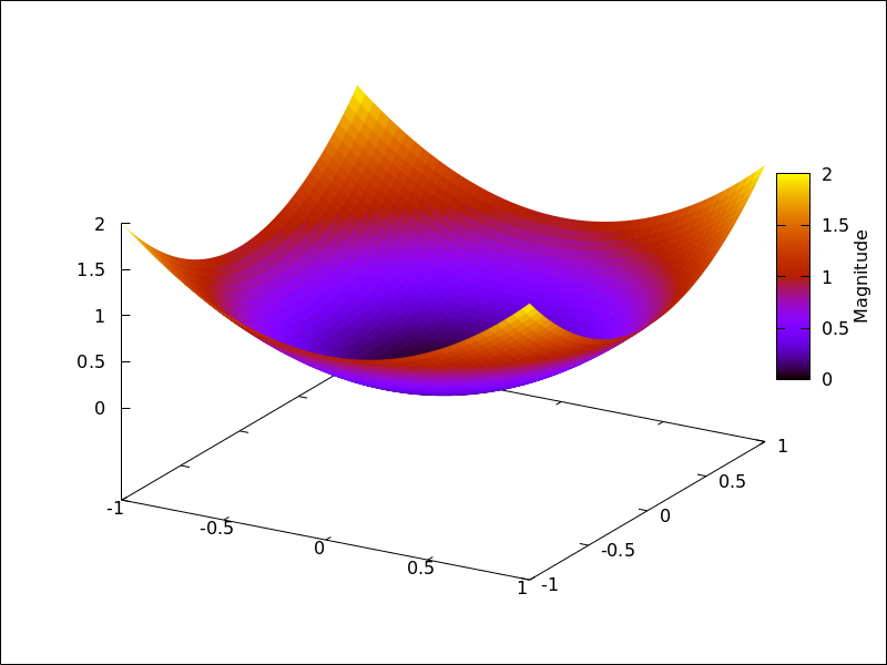
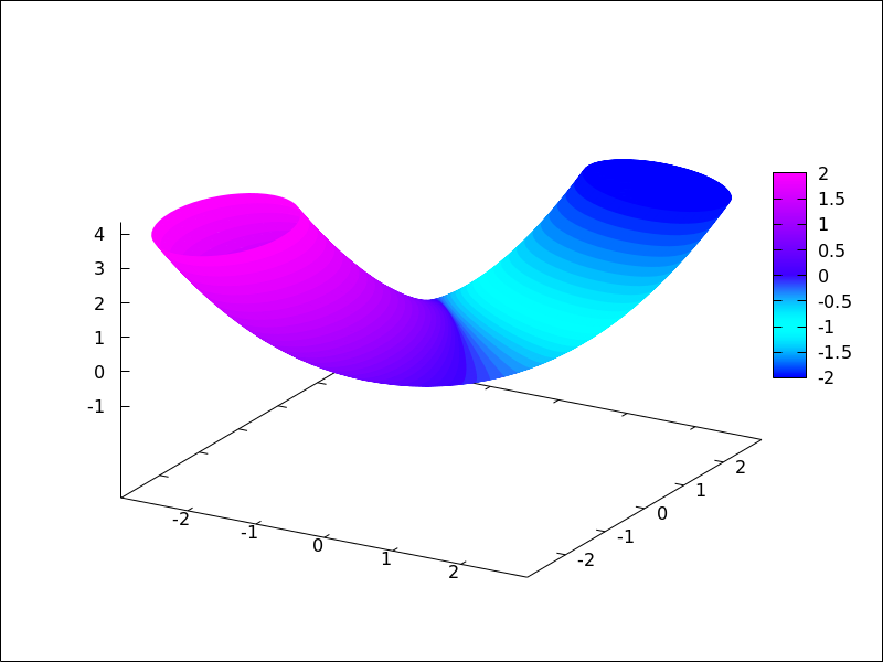
 Color scale and 3D coloured object.
(%i1) draw3d(
        colorbox   = "Magnitude",
        enhanced3d = true,
        explicit(x^2+y^2,x,-1,1,y,-1,1))$
See also palette_005fdraw.
See also: palette_draw.
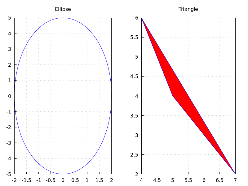
columns — Variable
Default value: 1
columns is the number of columns in multiple plots.
Since this is a global graphics option, its position in the scene description
does not matter. It can be also used as an argument of function draw.
Example:
(%i1) scene1: gr2d(title="Ellipse",
                   nticks=30,
                   parametric(2*cos(t),5*sin(t),t,0,2*%pi))$
(%i2) scene2: gr2d(title="Triangle",
                   polygon([4,5,7],[6,4,2]))$
(%i3) draw(scene1, scene2, columns = 2)$

contour — Variable
Default value: none
Option contour enables the user to select where to plot contour lines.
Possible values are:
none:
no contour lines are plotted.
base:
contour lines are projected on the xy plane.
surface:
contour lines are plotted on the surface.
both:
two contour lines are plotted: on the xy plane and on the surface.
map:
contour lines are projected on the xy plane, and the view point is
set just in the vertical.
Since this is a global graphics option, its position in the scene description does not matter.
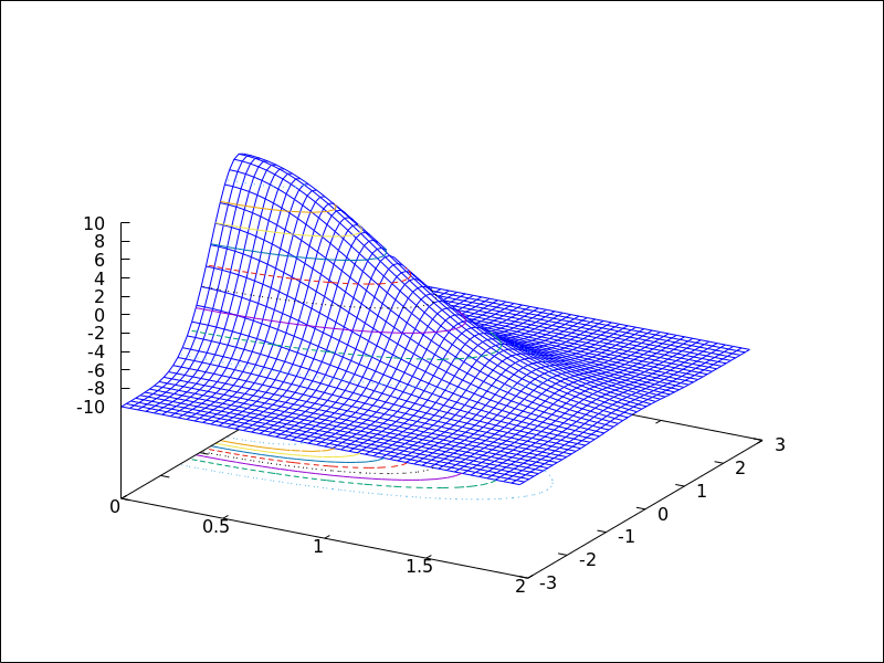
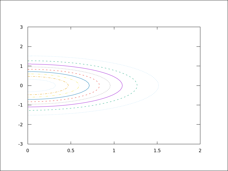
Example:
(%i1) draw3d(explicit(20*exp(-x^2-y^2)-10,x,0,2,y,-3,3),
             contour_levels = 15,
             contour        = both,
             surface_hide   = true) $
(%i1) draw3d(explicit(20*exp(-x^2-y^2)-10,x,0,2,y,-3,3),
             contour_levels = 15,
             contour        = map
      ) $
contour_levels — Variable
Default value: 5
This graphic option controls the way contours are drawn.
contour_levels can be set to a positive integer number, a list of three
numbers or an arbitrary set of numbers:
When option contour_levels is bounded to positive integer n,
n contour lines will be drawn at equal intervals. By default, five
equally spaced contours are plotted.
When option contour_levels is bounded to a list of length three of the
form [lowest,s,highest], contour lines are plotted from lowest
to highest in steps of s.
When option contour_levels is bounded to a set of numbers of the
form {n1, n2, ...}, contour lines are plotted at values n1,
n2, …
Since this is a global graphics option, its position in the scene description does not matter.
Examples:
Ten equally spaced contour lines. The actual number of levels can be adjusted to give simple labels.
(%i1) draw3d(color = green,
             explicit(20*exp(-x^2-y^2)-10,x,0,2,y,-3,3),
             contour_levels = 10,
             contour        = both,
             surface_hide   = true) $
From -8 to 8 in steps of 4.
(%i1) draw3d(color = green,
             explicit(20*exp(-x^2-y^2)-10,x,0,2,y,-3,3),
             contour_levels = [-8,4,8],
             contour        = both,
             surface_hide   = true) $
Isolines at levels -7, -6, 0.8 and 5.
(%i1) draw3d(color = green,
             explicit(20*exp(-x^2-y^2)-10,x,0,2,y,-3,3),
             contour_levels = {-7, -6, 0.8, 5},
             contour        = both,
             surface_hide   = true) $
See also contour.
See also: contour.
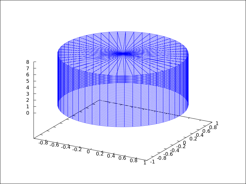
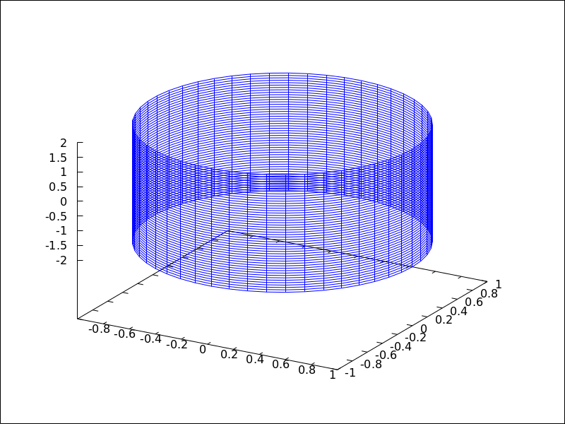
cylindrical (radius, z, minz, maxz, azi, minazi, maxazi) — Function
Draws 3D functions defined in cylindrical coordinates.
3D
cylindrical(radius, z, minz, maxz, azi, minazi, maxazi) plots the function radius(z, azi) defined in cylindrical coordinates, with variable z taking
values from minz to maxz and azimuth azi taking values
from minazi to maxazi.
This object is affected by the following graphic options: xu_grid,
yv_grid, line_type, key, wired_surface, enhanced3d and color
Example:
(%i1) draw3d(cylindrical(1,z,-2,2,az,0,2*%pi))$
See also: xu_grid, yv_grid, line_type, key, wired_surface.
data_file_name — Variable
Default value: "data.gnuplot"
This is the name of the file with the numeric data needed by Gnuplot to build the requested plot.
Since this is a global graphics option, its position in the scene description
does not matter. It can be also used as an argument of function draw.
See example in gnuplot_file_name.
delay — Variable
Default value: 5
This is the delay in 1/100 seconds of frames in animated gif files.
Since this is a global graphics option, its position in the scene description
does not matter. It can be also used as an argument of function draw.
Example:
(%i1) draw(
        delay     = 100,
        file_name = "zzz",
        terminal  = 'animated_gif,
        gr2d(explicit(x^2,x,-1,1)),
        gr2d(explicit(x^3,x,-1,1)),
        gr2d(explicit(x^4,x,-1,1)));
End of animation sequence
(%o2)          [gr2d(explicit), gr2d(explicit), gr2d(explicit)]
Option delay is only active in animated gif’s; it is ignored in
any other case.
See also terminal, and dimensions.
See also: terminal.
dimensions — Variable
Default value: [600,500]
Dimensions of the output terminal. Its value is a list formed by the width and the height. The meaning of the two numbers depends on the terminal you are working with.
With terminals gif, animated_gif, png, jpg,
svg, screen, wxt, qt, x11,
windows and aquaterm, the integers represent the number of
points in each direction. If they are not integers, they are rounded.
With terminals eps, epslatex, epslatex_standalone,
eps_color, multipage_eps, multipage_eps_color,
cairolatex_pdf, cairolatex_pdf_standalone,
pdf, multipage_pdf, pdfcairo,
multipage_pdfcairo, tikz, and tikz_standalone, both
numbers represent hundredths of cm, which means that, by default,
pictures in these formats are 6 cm in width and 5 cm in height.
Since this is a global graphics option, its position in the scene description
does not matter. It can be also used as an argument of function draw.
Examples:
Option dimensions applied to file output
and to wxt canvas.
(%i1) draw2d(
        dimensions = [300,300],
        terminal   = 'png,
        explicit(x^4,x,-1,1)) $
(%i2) draw2d(
        dimensions = [300,300],
        terminal   = 'wxt,
        explicit(x^4,x,-1,1)) $
Option dimensions applied to eps output.
We want an eps file with A4 portrait dimensions.
(%i1) A4portrait: 100*[21, 29.7]$
(%i2) draw3d(
        dimensions = A4portrait,
        terminal   = 'eps,
        explicit(x^2-y^2,x,-2,2,y,-2,2)) $
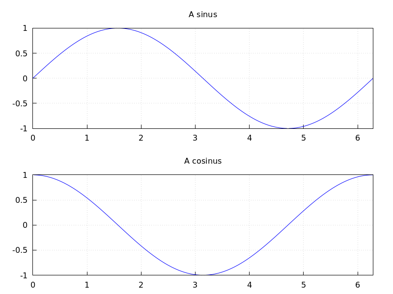
draw (<arg_1>, …) — Function
Plots a series of scenes; its arguments are gr2d and/or gr3d
objects, together with some options, or lists of scenes and options.
By default, the scenes are put together
in one column.
Besides scenes the function draw accepts the following global options:
terminal, columns, dimensions, file_name
and delay.
Functions draw2d and draw3d short cuts that can be used
when only one scene is required, in two or three dimensions, respectively.
See also gr2d and gr3d.
Examples:
(%i1) scene1: gr2d(title="Ellipse",
                   nticks=300,
                   parametric(2*cos(t),5*sin(t),t,0,2*%pi))$
(%i2) scene2: gr2d(title="Triangle",
                   polygon([4,5,7],[6,4,2]))$
(%i3) draw(scene1, scene2, columns = 2)$
(%i1) scene1: gr2d(title="A sinus",
        grid=true,
        explicit(sin(t),t,0,2*%pi))$
(%i2) scene2: gr2d(title="A cosinus",
        grid=true,
        explicit(cos(t),t,0,2*%pi))$
(%i3) draw(scene1, scene2)$
The following two draw sentences are equivalent:
(%i1) draw(gr3d(explicit(x^2+y^2,x,-1,1,y,-1,1)));
(%o1)                          [gr3d(explicit)]
(%i2) draw3d(explicit(x^2+y^2,x,-1,1,y,-1,1));
(%o2)                          [gr3d(explicit)]
Creating an animated gif file:
(%i1) draw(
        delay     = 100,
        file_name = "zzz",
        terminal  = 'animated_gif,
        gr2d(explicit(x^2,x,-1,1)),
        gr2d(explicit(x^3,x,-1,1)),
        gr2d(explicit(x^4,x,-1,1)));
End of animation sequence
(%o1)          [gr2d(explicit), gr2d(explicit), gr2d(explicit)]
 See also
 gr2d, gr3d, draw2d and draw3d.
See also: terminal, columns, dimensions, file_name, delay, draw2d, draw3d, gr2d, gr3d.
draw2d (argument_1, …) — Function
This function is a shortcut for
draw(gr2d(options, ..., graphic_object, ...)).
It can be used to plot a unique scene in 2d, as can be seen in most examples below.
See also draw and gr2d.
See also: draw, gr2d.
draw3d (argument_1, …) — Function
This function is a shortcut for
draw(gr3d(options, ..., graphic_object, ...)).
It can be used to plot a unique scene in 3d, as can be seen in many examples below.
See also draw and gr3d.
See also: draw, gr3d.
draw_file (graphic option, …, graphic object, …) — Function
Saves the current plot into a file. Accepted graphics options are:
terminal, dimensions and file_name.
Example:
(%i1) /* screen plot */
      draw(gr3d(explicit(x^2+y^2,x,-1,1,y,-1,1)))$
(%i2) /* same plot in eps format */
      draw_file(terminal  = eps,
                dimensions = [5,5]) $
draw_realpart — Variable
Default value: true
When true, functions to be drawn are considered as complex functions whose
real part value should be plotted; when false, nothing will be plotted when
the function does not give a real value.
This option affects objects explicit and parametric in 2D and 3D, and
parametric_005fsurface.
Example:
(%i1) draw2d(
        draw_realpart = false,
        explicit(sqrt(x^2  - 4*x) - x, x, -1, 5),
        color         = red,
        draw_realpart = true,
        parametric(x,sqrt(x^2  - 4*x) - x + 1, x, -1, 5) );
See also: explicit, parametric, parametric_surface.
draw_renderer — Variable
Default value: gnuplot_pipes
The only permitted values are gnuplot_pipes, gnuplot,
vtk, vtk6 or vtk7. When draw_renderer is set
to vtk, the VTK interface is used for draw.
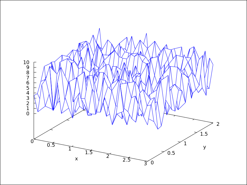
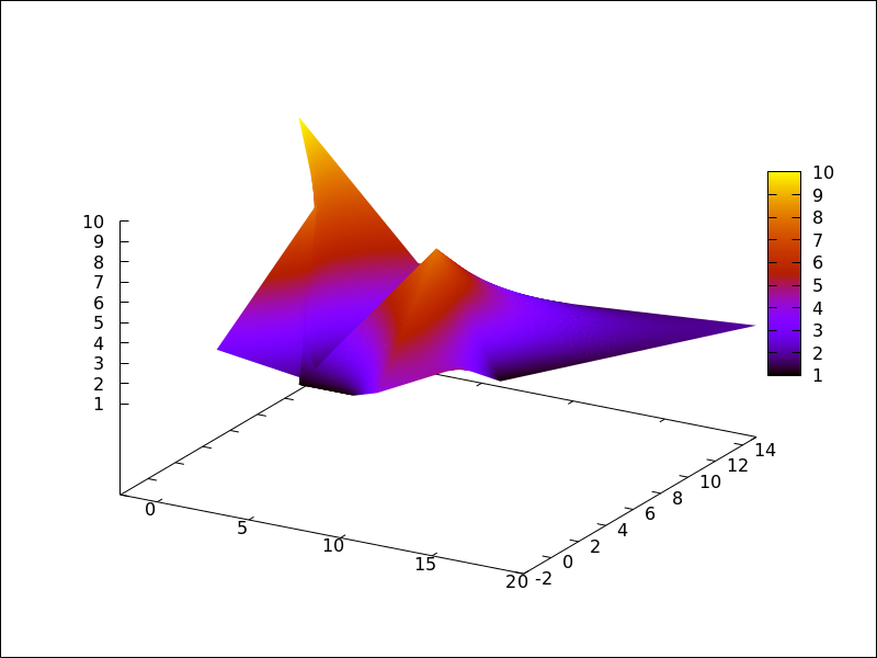
elevation_grid (mat, x0, y0, width, height) — Function
Draws matrix mat in 3D space. z values are taken from mat, the abscissas range from x0 to $x0 + width$ and ordinates from y0 to $y0 + height$. Element $a(1,1)$ is projected on point $(x0,y0+height)$, $a(1,n)$ on $(x0+width,y0+height)$, $a(m,1)$ on $(x0,y0)$, and $a(m,n)$ on $(x0+width,y0)$.
This object is affected by the following graphic options: line_type,,
line_width key, wired_surface, enhanced3d and color
In older versions of Maxima, elevation_grid was called mesh.
See also mesh.
Example:
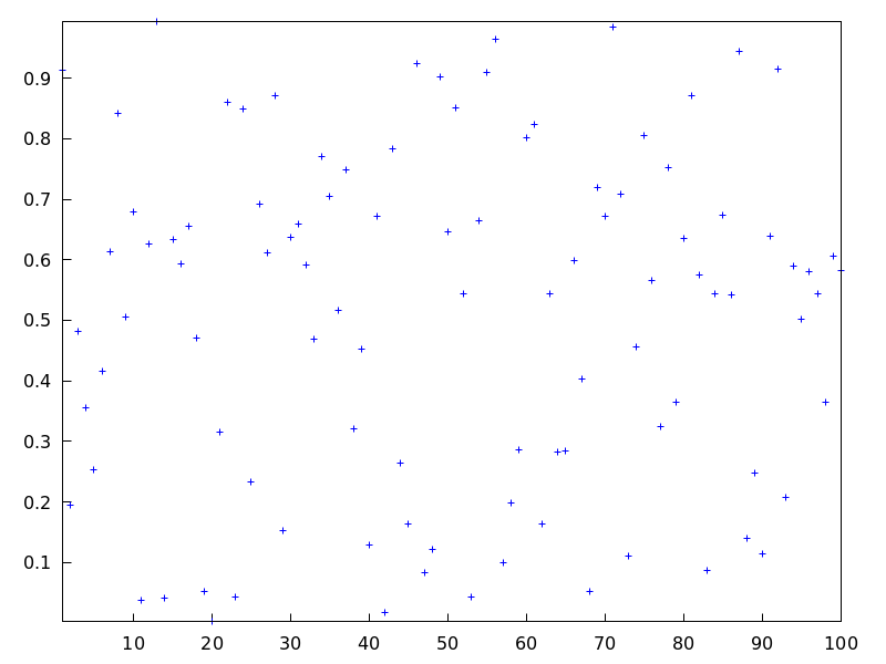
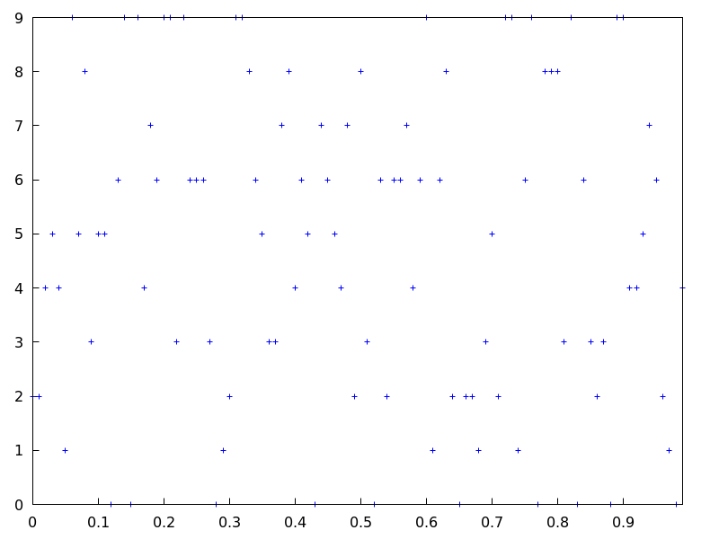
(%i1) m: apply(
            matrix,
            makelist(makelist(random(10.0),k,1,30),i,1,20)) $
(%i2) draw3d(
         color = blue,
         elevation_grid(m,0,0,3,2),
         xlabel = "x",
         ylabel = "y",
         surface_hide = true);
See also: line_type, line_width, key, wired_surface, enhanced3d, elevation_grid, mesh.
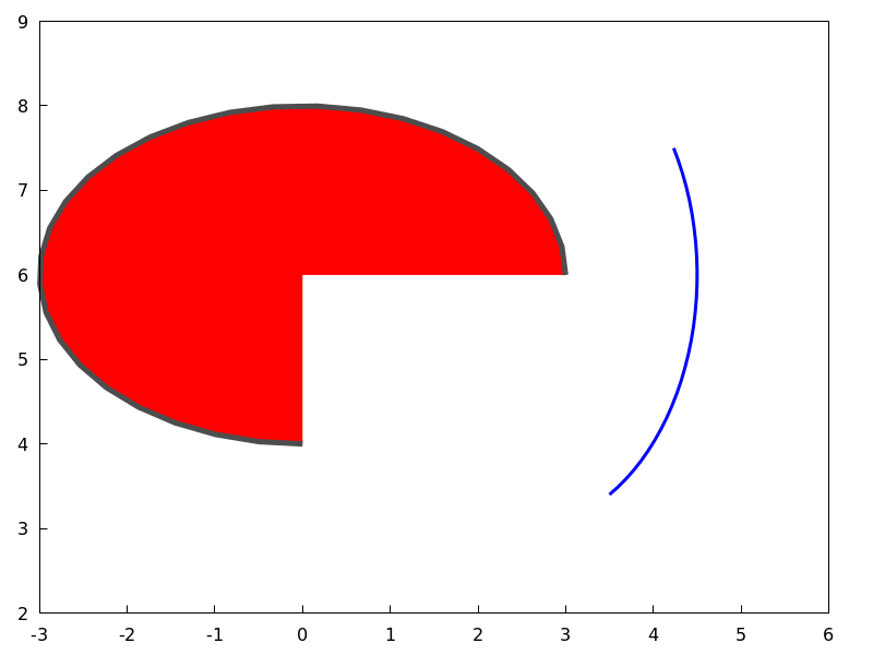
ellipse (xc, yc, a, b, ang1, ang2) — Function
Draws ellipses and circles in 2D.
2D
ellipse (xc, yc, a, b, ang1, ang2)
plots an ellipse centered at [xc, yc] with horizontal and vertical
semi axis a and b, respectively, starting at angle ang1 with an amplitude
equal to angle ang2.
This object is affected by the following graphic options: nticks,
transparent, fill_color, fill_density, border, line_width,
line_type, key and color
Example:
(%i1) draw2d(transparent = false,
             fill_color  = red,
             color       = gray30,
             transparent = false,
             line_width  = 5,
             ellipse(0,6,3,2,270,-270),
             /* center (x,y), a, b, start & end in degrees */
             transparent = true,
             color       = blue,
             line_width  = 3,
             ellipse(2.5,6,2,3,30,-90),
             xrange      = [-3,6],
             yrange      = [2,9] )$
See also: nticks, transparent, fill_color, fill_density, border, line_type, key.
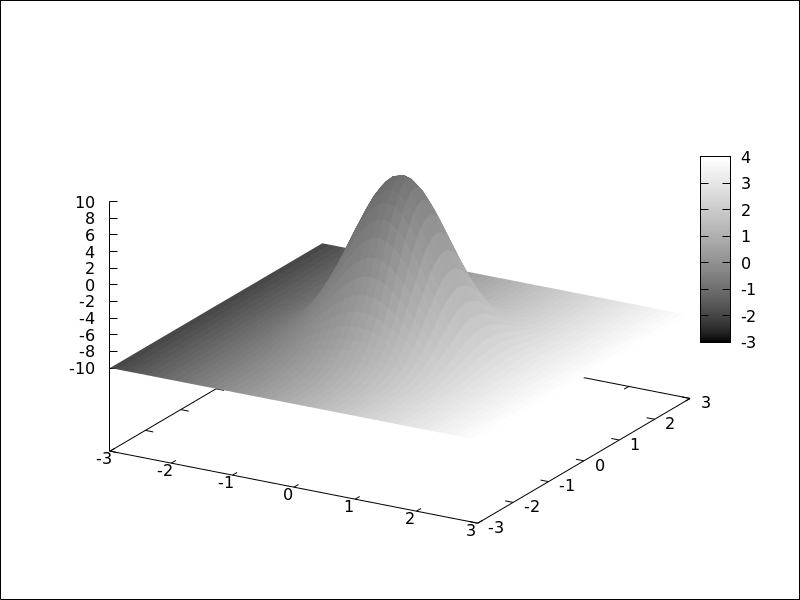
enhanced3d — Variable
Default value: none
If enhanced3d is none, surfaces are not colored in 3D plots.
In order to get a colored surface, a list must be assigned to option
enhanced3d, where the first element is an expression and the rest
are the names of the variables or parameters used in that expression. A list such
[f(x,y,z), x, y, z] means that point [x,y,z] of the surface
is assigned number f(x,y,z), which will be colored according to
the actual palette. For those 3D graphic objects defined in terms of
parameters, it is possible to define the color number in terms of
the parameters, as in [f(u), u], as in objects parametric and
tube, or [f(u,v), u, v], as in object parametric_surface.
While all 3D objects admit the model based on absolute coordinates,
[f(x,y,z), x, y, z], only two of them, namely explicit
and elevation_grid, accept also models defined on the [x,y] coordinates,
[f(x,y), x, y]. 3D graphic object implicit accepts only the
[f(x,y,z), x, y, z] model. Object points accepts also the
[f(x,y,z), x, y, z] model, but when points have a chronological nature,
model [f(k), k] is also valid, being k an ordering parameter.
When enhanced3d is assigned something different to none, options
color and surface_hide are ignored.
The names of the variables defined in the lists may be different to those used in the definitions of the graphic objects.
In order to maintain back compatibility, enhanced3d = false is equivalent
to enhanced3d = none, and enhanced3d = true is equivalent to
enhanced3d = [z, x, y, z]. If an expression is given to enhanced3d,
its variables must be the same used in the surface definition. This is not
necessary when using lists.
See option palette to learn how palettes are specified.
Examples:
explicit object with coloring defined by the [f(x,y,z), x, y, z] model.
(%i1) draw3d(
         enhanced3d = [x-z/10,x,y,z],
         palette    = gray,
         explicit(20*exp(-x^2-y^2)-10,x,-3,3,y,-3,3))$
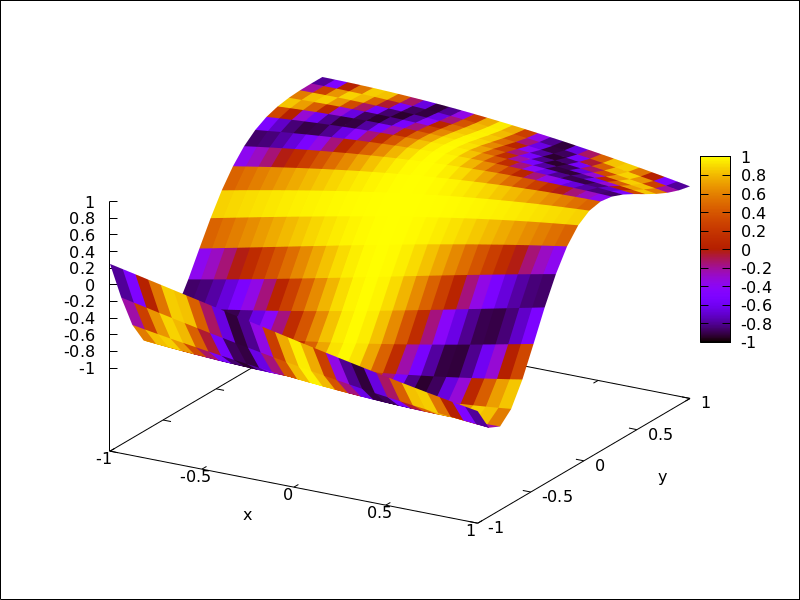
explicit object with coloring defined by the [f(x,y), x, y] model.
The names of the variables defined in the lists may be different to those
used in the definitions of the graphic objects; in this case, r corresponds
to x, and s to y.
(%i1) draw3d(
         enhanced3d = [sin(r*s),r,s],
         explicit(20*exp(-x^2-y^2)-10,x,-3,3,y,-3,3))$

parametric object with coloring defined by the [f(x,y,z), x, y, z] model.
(%i1) draw3d(
         nticks = 100,
         line_width = 2,
         enhanced3d = [if y>= 0 then 1 else 0, x, y, z],
         parametric(sin(u)^2,cos(u),u,u,0,4*%pi)) $
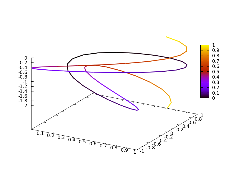
parametric object with coloring defined by the [f(u), u] model.
In this case, (u-1)^2 is a shortcut for [(u-1)^2,u].
(%i1) draw3d(
         nticks = 60,
         line_width = 3,
         enhanced3d = (u-1)^2,
         parametric(cos(5*u)^2,sin(7*u),u-2,u,0,2))$
elevation_grid object with coloring defined by the [f(x,y), x, y] model.
(%i1) m: apply(
           matrix,
           makelist(makelist(cos(i^2/80-k/30),k,1,30),i,1,20)) $
(%i2) draw3d(
         enhanced3d = [cos(x*y*10),x,y],
         elevation_grid(m,-1,-1,2,2),
         xlabel = "x",
         ylabel = "y");
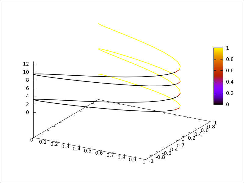
tube object with coloring defined by the [f(x,y,z), x, y, z] model.
(%i1) draw3d(
         enhanced3d = [cos(x-y),x,y,z],
         palette = gray,
         xu_grid = 50,
         tube(cos(a), a, 0, 1, a, 0, 4*%pi) )$
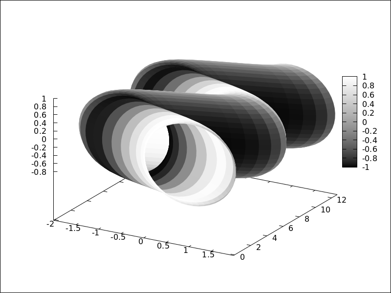
tube object with coloring defined by the [f(u), u] model.
Here, enhanced3d = -a would be the shortcut for enhanced3d = [-foo,foo].
(%i1) draw3d(
         capping = [true, false],
         palette = [26,15,-2],
         enhanced3d = [-foo, foo],
         tube(a, a, a^2, 1, a, -2, 2) )$
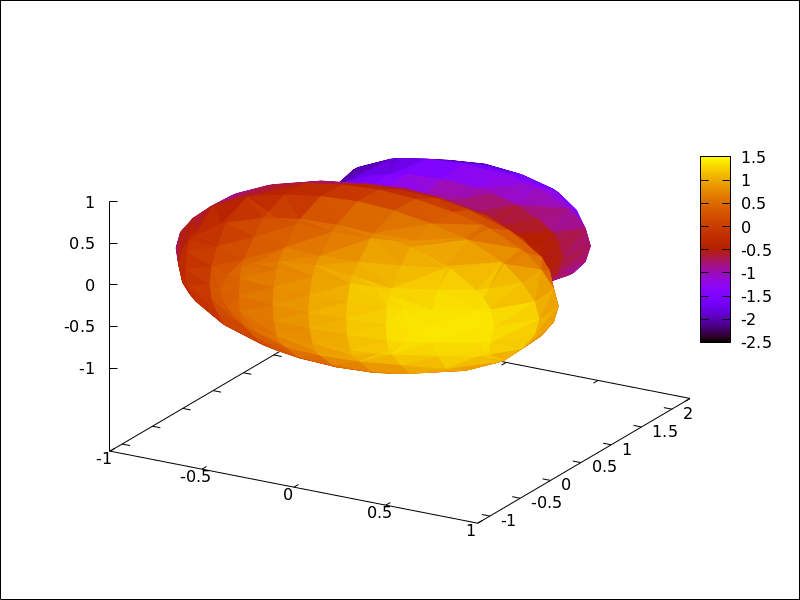
implicit and points objects with coloring defined by the [f(x,y,z), x, y, z] model.
(%i1) draw3d(
enhanced3d = [x-y,x,y,z],
implicit((x^2+y^2+z^2-1)*(x^2+(y-1.5)^2+z^2-0.5)=0.015,
x,-1,1,y,-1.2,2.3,z,-1,1)) $
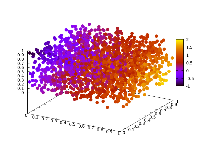
(%i2) m: makelist([random(1.0),random(1.0),random(1.0)],k,1,2000)$
(%i3) draw3d(
         point_type = filled_circle,
         point_size = 2,
         enhanced3d = [u+v-w,u,v,w],
         points(m) ) $
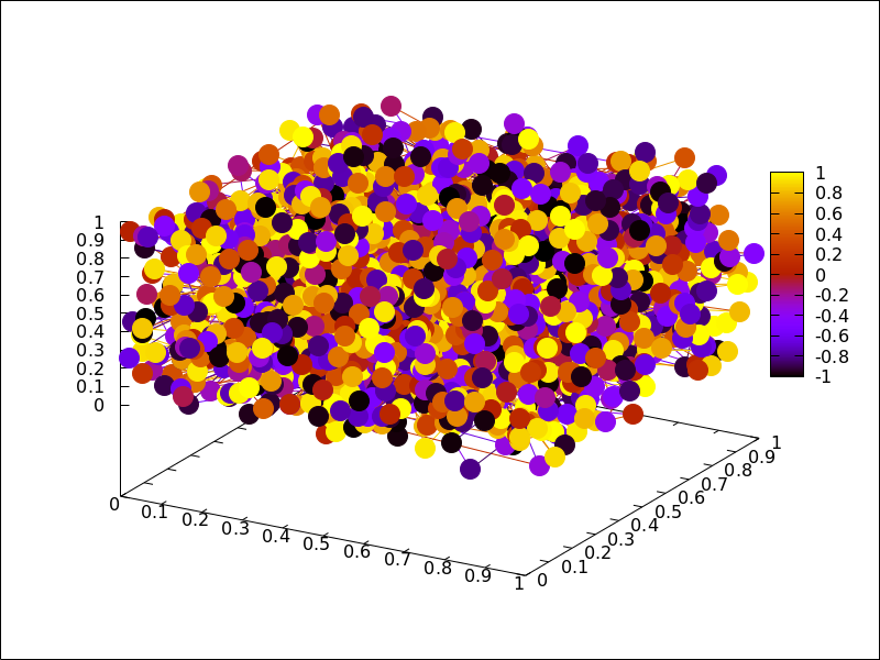
When points have a chronological nature, model [f(k), k] is also valid,
being k an ordering parameter.
(%i1) m:makelist([random(1.0), random(1.0), random(1.0)],k,1,5)$
(%i2) draw3d(
         enhanced3d = [sin(j), j],
         point_size = 3,
         point_type = filled_circle,
         points_joined = true,
         points(m)) $
See also: enhanced3d, parametric, tube, elevation_grid.
error_type — Variable
Default value: y
Depending on its value, which can be x, y, or xy,
graphic object errors will draw points with horizontal, vertical,
or both, error bars. When error_type=boxes, boxes will be drawn
instead of crosses.
See also errors.
See also: errors.
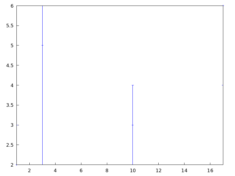
errors ([x1, x2, …], [y1, y2, …]) — Function
Draws points with error bars, horizontally, vertically or both, depending on the
value of option error_type.
2D
If error_type = x, arguments to errors must be of the form
[x, y, xdelta] or [x, y, xlow, xhigh]. If error_type = y,
arguments must be of the form [x, y, ydelta] or
[x, y, ylow, yhigh]. If error_type = xy or
error_type = boxes, arguments to errors must be of the form
[x, y, xdelta, ydelta] or [x, y, xlow, xhigh, ylow, yhigh].
See also error_005ftype.
This object is affected by the following graphic options: error_type,points_joined, line_width, key, line_type,color fill_density, xaxis_secondary and yaxis_005fsecondary.
Option fill_density is only relevant when error_type=boxes.
Examples:
Horizontal error bars.
(%i1) draw2d(
        error_type = 'y,
        errors([[1,2,1], [3,5,3], [10,3,1], [17,6,2]]))$
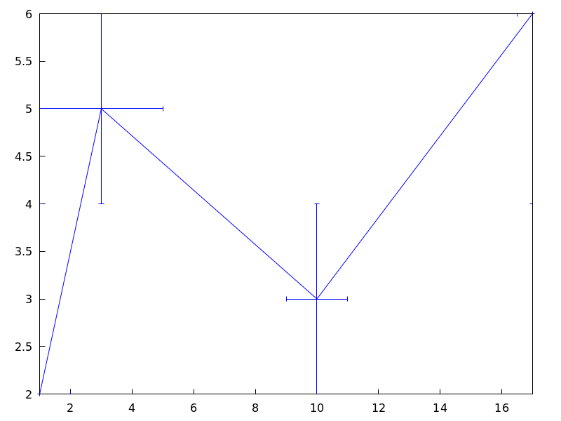
Vertical and horizontal error bars.
(%i1) draw2d(
        error_type = 'xy,
        points_joined = true,
        color = blue,
        errors([[1,2,1,2], [3,5,2,1], [10,3,1,1], [17,6,1/2,2]]));
See also: error_type, points_joined, line_width, key, line_type, fill_density, xaxis_secondary, yaxis_secondary.
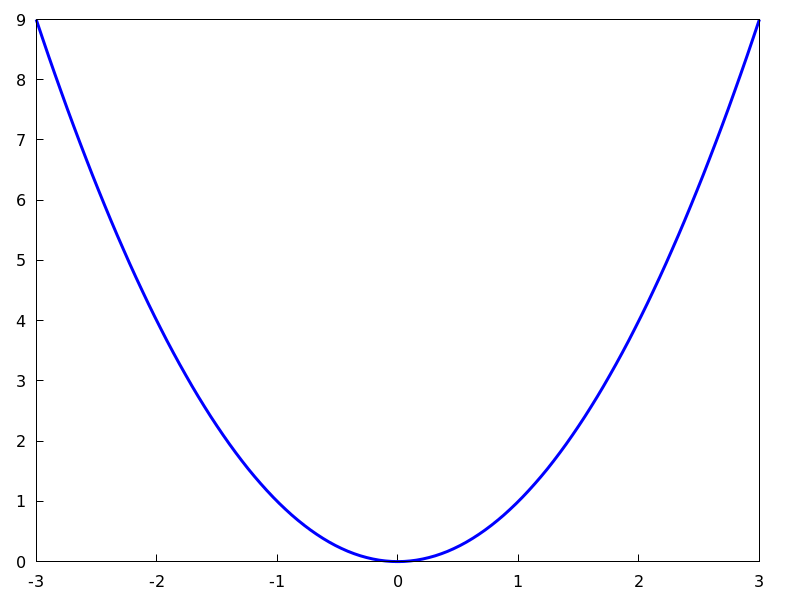
explicit (expr, var, minval, maxval) — Function
Draws explicit functions in 2D and 3D.
2D
explicit(fcn,var,minval,maxval) plots explicit function fcn,
with variable var taking values from minval to maxval.
This object is affected by the following graphic options: nticks,
adapt_depth, draw_realpart, line_width, line_type, key,
filled_func, fill_color, fill_density, and color
Example:
(%i1) draw2d(line_width = 3,
             color      = blue,
             explicit(x^2,x,-3,3) )$
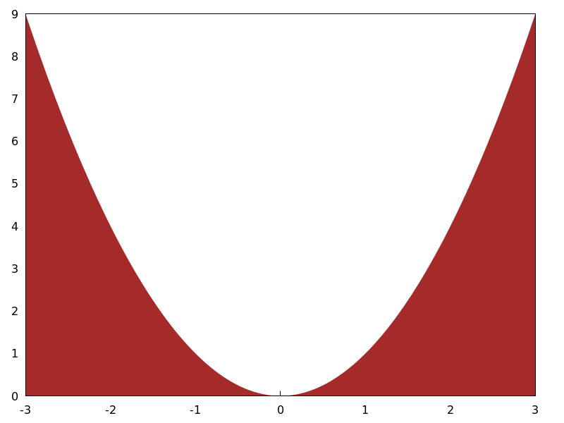
(%i2) draw2d(fill_color  = brown,
             filled_func = true,
             explicit(x^2,x,-3,3) )$
3D
explicit(fcn, var1, minval1, maxval1, var2, minval2, maxval2) plots the explicit function fcn, with
variable var1 taking values from minval1 to maxval1 and
variable var2 taking values from minval2 to maxval2.
This object is affected by the following graphic options: draw_realpart, xu_grid,
yv_grid, line_type, line_width, key, wired_surface,
enhanced3d and color.
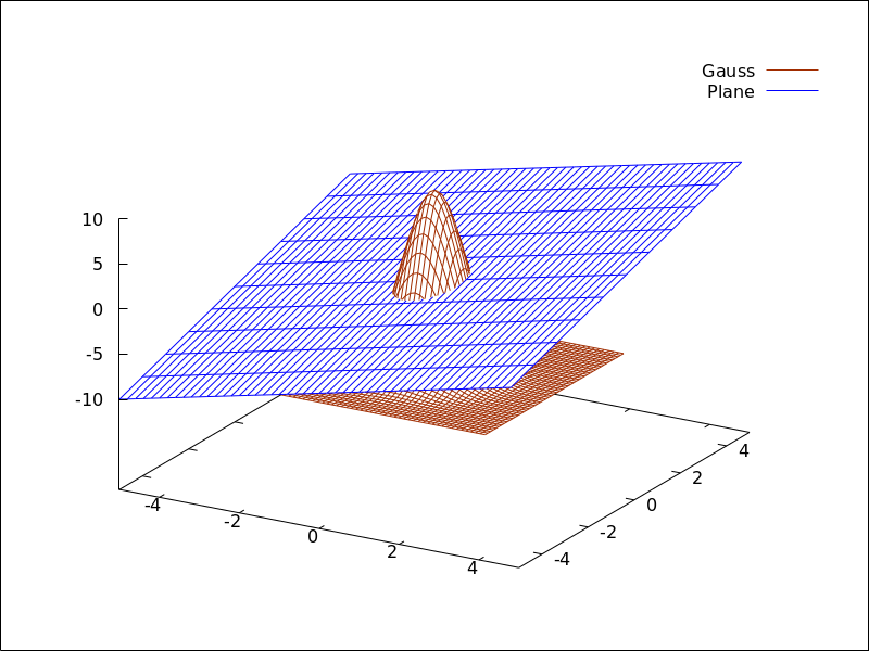
Example:
(%i1) draw3d(key   = "Gauss",
             color = "#a02c00",
             explicit(20*exp(-x^2-y^2)-10,x,-3,3,y,-3,3),
             yv_grid     = 10,
             color = blue,
             key   = "Plane",
             explicit(x+y,x,-5,5,y,-5,5),
             surface_hide = true)$
See also filled_func for filled functions.
See also: nticks, draw_realpart, line_width, line_type, key, filled_func, fill_color, fill_density, xu_grid, yv_grid, wired_surface, enhanced3d.
file_name — Variable
Default value: "maxima_out"
This is the name of the file where terminals png, jpg, gif,
eps, eps_color, pdf, pdfcairo and svg
will save the graphic.
Since this is a global graphics option, its position in the scene description
does not matter. It can be also used as an argument of function draw.
Example:
(%i1) draw2d(file_name = "myfile",
             explicit(x^2,x,-1,1),
             terminal  = 'png)$
See also terminal, dimensions_005fdraw.
See also: terminal, dimensions_draw.
fill_color — Variable
Default value: "red"
fill_color specifies the color for filling polygons and
2d explicit functions.
See color to learn how colors are specified.
fill_density — Variable
Default value: 0
fill_density is a number between 0 and 1 that specifies
the intensity of the fill_color in bars objects.
See bars for examples.
filled_func — Variable
Default value: false
Option filled_func controls how regions limited by functions
should be filled. When filled_func is true, the region
bounded by the function defined with object explicit and the
bottom of the graphic window is filled with fill_color. When
filled_func contains a function expression, then the region bounded
by this function and the function defined with object explicit
will be filled. By default, explicit functions are not filled.
A useful special case is filled_func=0, which generates the region
bond by the horizontal axis and the explicit function.
This option affects only the 2d graphic object explicit.
Example:
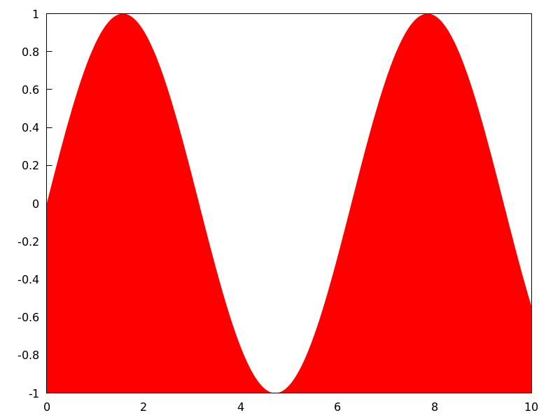
Region bounded by an explicit object and the bottom of the
graphic window.
(%i1) draw2d(fill_color  = red,
             filled_func = true,
             explicit(sin(x),x,0,10) )$
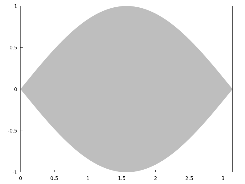
Region bounded by an explicit object and the function
defined by option filled_func. Note that the variable in
filled_func must be the same as that used in explicit.
(%i1) draw2d(fill_color  = grey,
             filled_func = sin(x),
             explicit(-sin(x),x,0,%pi));
 See also
 fill_color and explicit.
See also: explicit, fill_color.
font — Variable
Default value: "" (empty string)
This option can be used to set the font face to be used by the terminal. Only one font face and size can be used throughout the plot.
Since this is a global graphics option, its position in the scene description does not matter.
See also font_005fsize.
Gnuplot doesn’t handle fonts by itself, it leaves this task to the support libraries of the different terminals, each one with its own philosophy about it. A brief summary follows:
x11: Uses the normal x11 font server mechanism.
Example:
(%i1) draw2d(font      = "Arial",
             font_size = 20,
             label(["Arial font, size 20",1,1]))$
windows: The windows terminal doesn’t support changing of fonts from inside the plot. Once the plot has been generated, the font can be changed right-clicking on the menu of the graph window.
png, jpeg, gif:
The libgd library uses the font path stored in the environment
variable GDFONTPATH; in this case, it is only necessary to
set option font to the font’s name. It is also possible to
give the complete path to the font file.
Examples:
Option font can be given the complete path to the font file:
(%i1) path: "/usr/share/fonts/truetype/freefont/" $
(%i2) file: "FreeSerifBoldItalic.ttf" $
(%i3) draw2d(
        font      = concat(path, file),
        font_size = 20,
        color     = red,
        label(["FreeSerifBoldItalic font, size 20",1,1]),
        terminal  = png)$
If environment variable GDFONTPATH is set to the
path where font files are allocated, it is possible to
set graphic option font to the name of the font.
(%i1) draw2d(
        font      = "FreeSerifBoldItalic",
        font_size = 20,
        color     = red,
        label(["FreeSerifBoldItalic font, size 20",1,1]),
        terminal  = png)$
Postscript:
Standard Postscript fonts are:
"Times-Roman", "Times-Italic", "Times-Bold",
"Times-BoldItalic",
"Helvetica", "Helvetica-Oblique", "Helvetica-Bold",
"Helvetic-BoldOblique", "Courier",
"Courier-Oblique", "Courier-Bold",
and "Courier-BoldOblique".
Example:
(%i1) draw2d(
        font      = "Courier-Oblique",
        font_size = 15,
        label(["Courier-Oblique font, size 15",1,1]),
        terminal = eps)$
pdf: Uses same fonts as Postscript.
pdfcairo: Uses same fonts as wxt.
wxt:
The pango library finds fonts via the fontconfig utility.
aqua:
Default is "Times-Roman".
The gnuplot documentation is an important source of information about terminals and fonts.
See also: font_size.
font_size — Variable
Default value: 10
This option can be used to set the font size to be used by the terminal.
Only one font face and size can be used throughout the plot. font_size is
active only when option font is not equal to the empty string.
Since this is a global graphics option, its position in the scene description does not matter.
See also font.
See also: font.
geomap (numlist) — Function
Draws cartographic maps in 2D and 3D.
2D
This function works together with global variable boundaries_array.
Argument numlist is a list containing numbers or lists of numbers.
All these numbers must be integers greater or equal than zero,
representing the components of global array boundaries_array.
Each component of boundaries_array is an array of floating
point quantities, the coordinates of a polygonal segment or map boundary.
geomap (numlist) flattens its arguments and draws the
associated boundaries in boundaries_array.
This object is affected by the following graphic options: line_width,
line_type and color.
Examples:
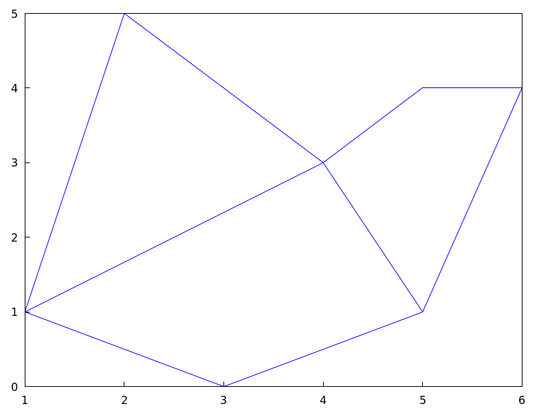
A simple map defined by hand:
(%i1) load("worldmap")$
(%i2) /* Vertices of boundary #0: {(1,1),(2,5),(4,3)} */
   ( bnd0: make_array(flonum,6),
     bnd0[0]:1.0, bnd0[1]:1.0, bnd0[2]:2.0,
     bnd0[3]:5.0, bnd0[4]:4.0, bnd0[5]:3.0 )$
(%i3) /* Vertices of boundary #1: {(4,3),(5,4),(6,4),(5,1)} */
   ( bnd1: make_array(flonum,8),
     bnd1[0]:4.0, bnd1[1]:3.0, bnd1[2]:5.0, bnd1[3]:4.0,
     bnd1[4]:6.0, bnd1[5]:4.0, bnd1[6]:5.0, bnd1[7]:1.0)$
(%i4) /* Vertices of boundary #2: {(5,1), (3,0), (1,1)} */
   ( bnd2: make_array(flonum,6),
     bnd2[0]:5.0, bnd2[1]:1.0, bnd2[2]:3.0,
     bnd2[3]:0.0, bnd2[4]:1.0, bnd2[5]:1.0 )$
(%i5) /* Vertices of boundary #3: {(1,1), (4,3)} */
   ( bnd3: make_array(flonum,4),
     bnd3[0]:1.0, bnd3[1]:1.0, bnd3[2]:4.0, bnd3[3]:3.0)$
(%i6) /* Vertices of boundary #4: {(4,3), (5,1)} */
   ( bnd4: make_array(flonum,4),
     bnd4[0]:4.0, bnd4[1]:3.0, bnd4[2]:5.0, bnd4[3]:1.0)$
(%i7) /* Pack all together in boundaries_array */
   ( boundaries_array: make_array(any,5),
     boundaries_array[0]: bnd0, boundaries_array[1]: bnd1,
     boundaries_array[2]: bnd2, boundaries_array[3]: bnd3,
     boundaries_array[4]: bnd4 )$
(%i8) draw2d(geomap([0,1,2,3,4]))$
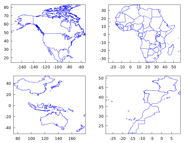
The auxiliary package worldmap sets the global variable
boundaries_array to real world boundaries in
(longitude, latitude) coordinates. These data are in the
public domain and come from
https://web.archive.org/web/20100310124019/http://www-cger.nies.go.jp/grid-e/gridtxt/grid19.html.
Package worldmap defines also boundaries for countries,
continents and coastlines as lists with the necessary components of
boundaries_array (see file share/draw/worldmap.mac
for more information). Package worldmap automatically loads
package worldmap.
(%i1) load("worldmap")$
(%i2) c1: gr2d(geomap([Canada,United_States,
Mexico,Cuba]))$
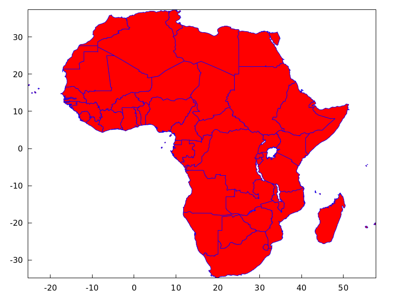
(%i3) c2: gr2d(geomap(Africa))$
(%i4) c3: gr2d(geomap([Oceania,China,Japan]))$
(%i5) c4: gr2d(geomap([France,Portugal,Spain,
Morocco,Western_Sahara]))$
(%i6) draw(columns = 2,
c1,c2,c3,c4)$
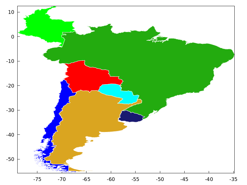
Package worldmap is also useful for plotting
countries as polygons. In this case, graphic object
geomap is no longer necessary and the polygon
object is used instead. Since lists are now used and not
arrays, maps rendering will be slower. See also make_poly_country
and make_poly_continent to understand the following code.
(%i1) load("worldmap")$
(%i2) mymap: append(
   [color      = white],  /* borders are white */
   [fill_color = red],             make_poly_country(Bolivia),
   [fill_color = cyan],            make_poly_country(Paraguay),
   [fill_color = green],           make_poly_country(Colombia),
   [fill_color = blue],            make_poly_country(Chile),
   [fill_color = "#23ab0f"],       make_poly_country(Brazil),
   [fill_color = goldenrod],       make_poly_country(Argentina),
   [fill_color = "midnight-blue"], make_poly_country(Uruguay))$
(%i3) apply(draw2d, mymap)$
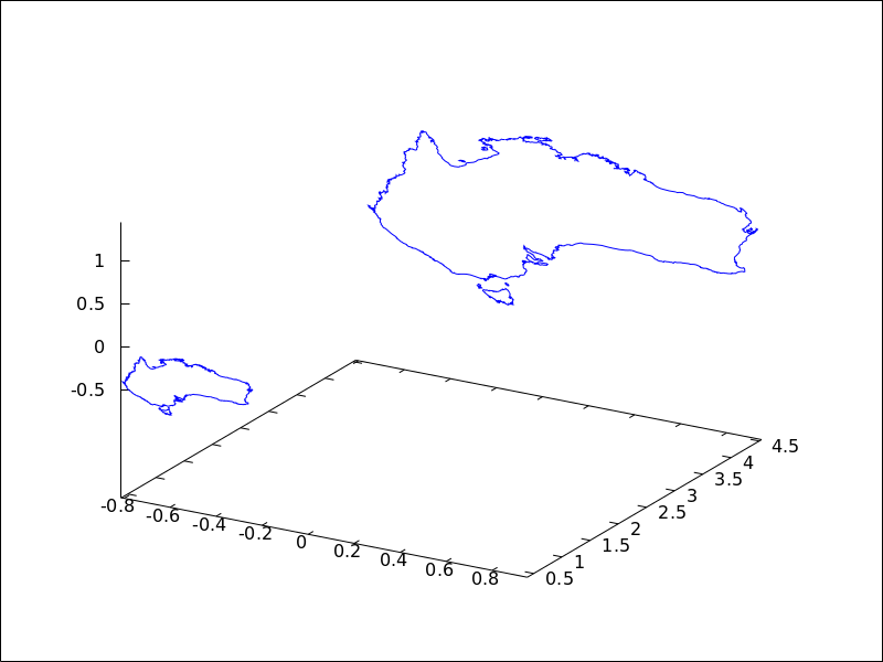
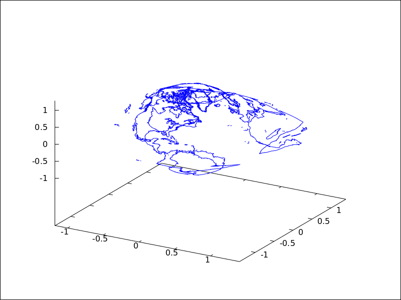
3D
geomap (numlist) projects map boundaries on the sphere of radius 1
centered at (0,0,0). It is possible to change the sphere or the projection type
by using geomap (numlist,3Dprojection).
Available 3D projections:
[spherical_projection,x,y,z,r]: projects map boundaries on the sphere of
radius r centered at (x,y,z).
(%i1) load("worldmap")$
(%i2) draw3d(geomap(Australia), /* default projection */
             geomap(Australia,
                    [spherical_projection,2,2,2,3]))$
[cylindrical_projection,x,y,z,r,rc]: re-projects spherical map boundaries on the cylinder of radius
rc and axis passing through the poles of the globe of radius r centered at (x,y,z).
(%i1) load("worldmap")$
(%i2) draw3d(geomap([America_coastlines,Eurasia_coastlines],
                    [cylindrical_projection,2,2,2,3,4]))$
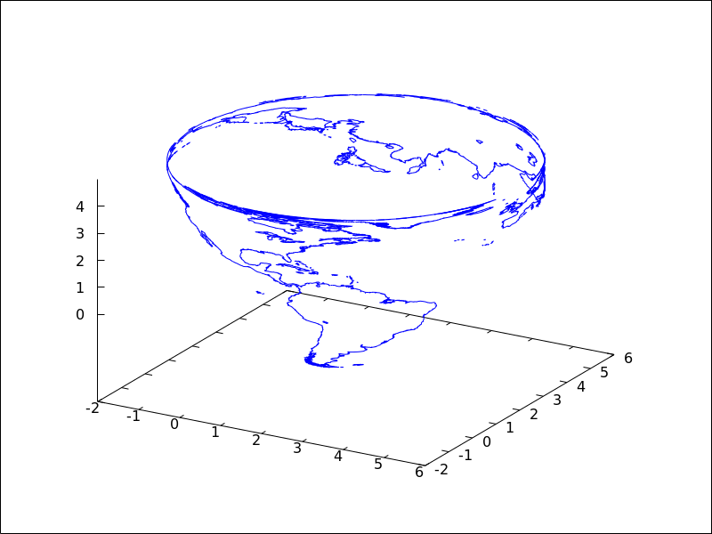
[conic_projection,x,y,z,r,alpha]: re-projects spherical map boundaries on the cones of angle alpha,
with axis passing through the poles of the globe of radius r centered at (x,y,z). Both
the northern and southern cones are tangent to sphere.
(%i1) load("worldmap")$
(%i2) draw3d(geomap(World_coastlines,
                    [conic_projection,0,0,0,1,90]))$
See also https://riotorto.users.sourceforge.net/Maxima/gnuplot/geomap/ for more elaborated examples.
See also: line_width, line_type, make_poly_country, make_poly_continent.
get_pixel (pic, x, y) — Function
Returns pixel from picture. Coordinates x and y range from 0 to
width-1 and height-1, respectively.
gnuplot_file_name — Variable
Default value: "maxout_xxx.gnuplot" with "xxx"
being a number that is unique to each concurrently-running
maxima process.
This is the name of the file with the necessary commands to be processed by Gnuplot.
Since this is a global graphics option, its position in the scene description
does not matter. It can be also used as an argument of function draw.
Example:
(%i1) draw2d(
       file_name = "my_file",
       gnuplot_file_name = "my_commands_for_gnuplot",
       data_file_name    = "my_data_for_gnuplot",
       terminal          = png,
       explicit(x^2,x,-1,1)) $
See also data_005ffile_005fname.
See also: data_file_name.
gr2d (argument_1, …) — Function
Function gr2d builds an object describing a 2D scene. Arguments are
graphic options, graphic objects, or lists containing both graphic options and objects.
This scene is interpreted sequentially: graphic options affect those graphic objects
placed on its right. Some graphic options affect the global appearance of the scene.
This is the list of graphic objects available for scenes in two dimensions:
bars, ellipse, explicit, image, implicit, label,
parametric, points, polar, polygon, quadrilateral,
rectangle, triangle, vector and geomap
(this one defined in package worldmap).
See also draw
and draw2d.
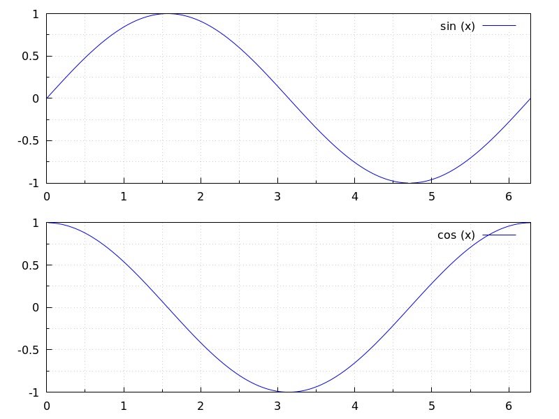
(%i1) draw(
    gr2d(
        key="sin (x)",grid=[2,2],
        explicit(
            sin(x),
            x,0,2*%pi
        )
    ),
    gr2d(
        key="cos (x)",grid=[2,2],
        explicit(
            cos(x),
            x,0,2*%pi
        )
    )
 );
(%o1)           [gr2d(explicit), gr2d(explicit)]
See also: bars, ellipse, explicit, image, implicit, label, parametric, points, polar, polygon, quadrilateral, rectangle, triangle, vector, draw, draw2d.
gr3d (argument_1, …) — Function
Function gr3d builds an object describing a 3d scene. Arguments are
graphic options, graphic objects, or lists containing both graphic options
and objects. This scene is interpreted sequentially: graphic options affect those
graphic objects placed on its right. Some graphic options affect the global
appearance of the scene.
This is the list of graphic objects available for scenes in three dimensions:
cylindrical, elevation_grid, explicit, implicit,
label, mesh, parametric,
parametric_surface, points, quadrilateral,
spherical, triangle, tube,
vector, and geomap (this one defined in package worldmap).
See also draw and draw3d.
See also: cylindrical, elevation_grid, explicit, implicit, label, mesh, parametric, parametric_surface, points, quadrilateral, spherical, triangle, tube, vector, geomap, draw, draw3d.
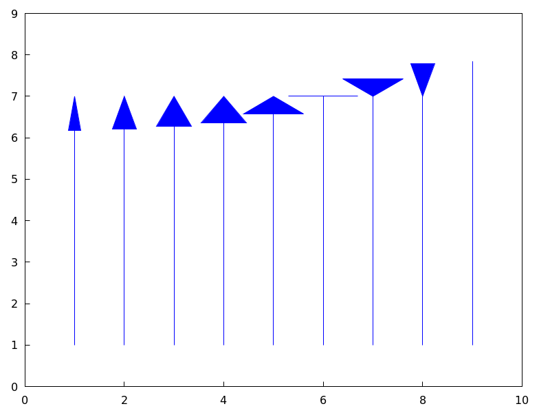
head_angle — Variable
Default value: 45
head_angle indicates the angle, in degrees, between the arrow heads and
the segment.
This option is relevant only for vector objects.
Example:
(%i1) draw2d(xrange      = [0,10],
             yrange      = [0,9],
             head_length = 0.7,
             head_angle  = 10,
             vector([1,1],[0,6]),
             head_angle  = 20,
             vector([2,1],[0,6]),
             head_angle  = 30,
             vector([3,1],[0,6]),
             head_angle  = 40,
             vector([4,1],[0,6]),
             head_angle  = 60,
             vector([5,1],[0,6]),
             head_angle  = 90,
             vector([6,1],[0,6]),
             head_angle  = 120,
             vector([7,1],[0,6]),
             head_angle  = 160,
             vector([8,1],[0,6]),
             head_angle  = 180,
             vector([9,1],[0,6]) )$
See also head_both, head_length, and head_005ftype.
See also: head_both, head_length, head_type.
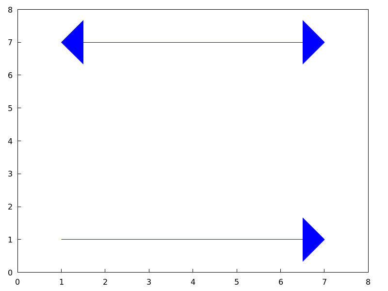
head_both — Variable
Default value: false
If head_both is true, vectors are plotted with two arrow heads.
If false, only one arrow is plotted.
This option is relevant only for vector objects.
Example:
(%i1) draw2d(xrange      = [0,8],
             yrange      = [0,8],
             head_length = 0.7,
             vector([1,1],[6,0]),
             head_both   = true,
             vector([1,7],[6,0]) )$
See also head_length, head_angle, and head_005ftype.
See also: head_length, head_angle, head_type.
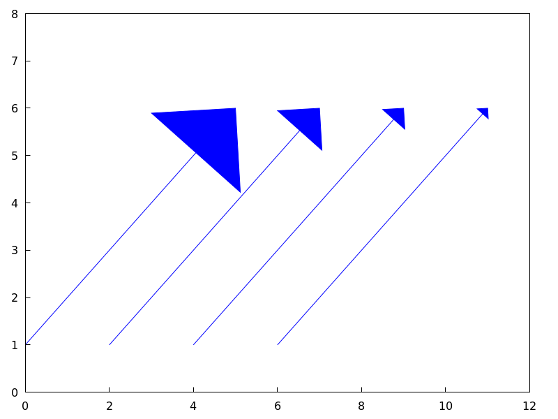
head_length — Variable
Default value: 2
head_length indicates, in x-axis units, the length of arrow heads.
This option is relevant only for vector objects.
Example:
(%i1) draw2d(xrange      = [0,12],
             yrange      = [0,8],
             vector([0,1],[5,5]),
             head_length = 1,
             vector([2,1],[5,5]),
             head_length = 0.5,
             vector([4,1],[5,5]),
             head_length = 0.25,
             vector([6,1],[5,5]))$
See also head_both, head_angle, and head_005ftype.
See also: head_both, head_angle, head_type.
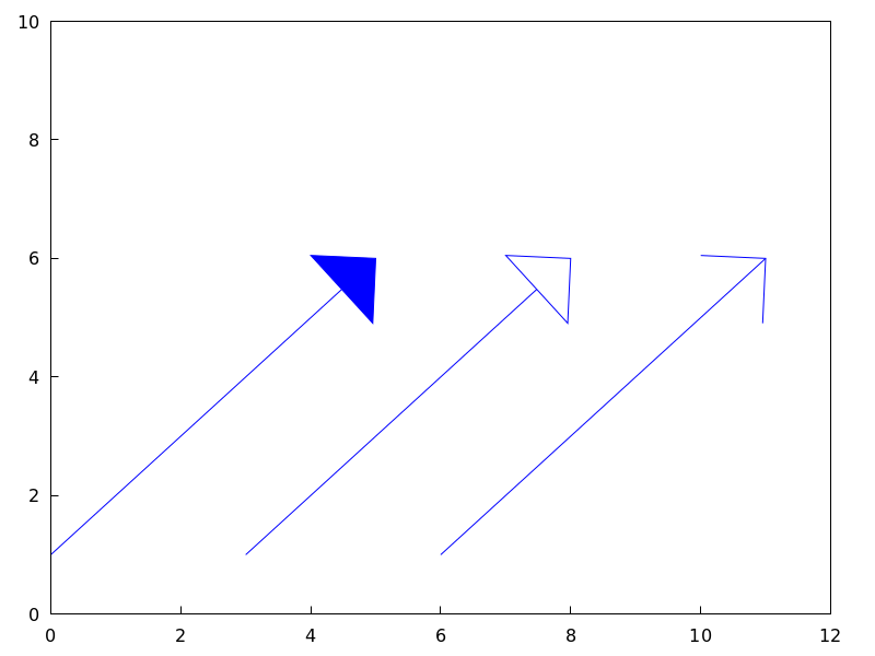
head_type — Variable
Default value: filled
head_type is used to specify how arrow heads are plotted. Possible
values are: filled (closed and filled arrow heads), empty
(closed but not filled arrow heads), and nofilled (open arrow heads).
This option is relevant only for vector objects.
Example:
(%i1) draw2d(xrange      = [0,12],
             yrange      = [0,10],
             head_length = 1,
             vector([0,1],[5,5]), /* default type */
             head_type = 'empty,
             vector([3,1],[5,5]),
             head_type = 'nofilled,
             vector([6,1],[5,5]))$
See also head_both, head_angle, and head_005flength.
See also: head_both, head_angle, head_length.
image (im, x0, y0, width, height) — Function
Renders images in 2D.
2D
image (im,x0,y0,width,height) plots image im in the rectangular
region from vertex (x0,y0) to (x0+width,y0+height) on the real
plane. Argument im must be a matrix of real numbers, a matrix of
vectors of length three or a picture object.
If im is a matrix of real numbers or a levels picture object,
pixel values are interpreted according to graphic option palette,
which is a vector of length three with components
ranging from -36 to +36; each value is an index for a formula mapping the levels
onto red, green and blue colors, respectively:
0: 0               1: 0.5           2: 1
 3: x               4: x^2           5: x^3
 6: x^4             7: sqrt(x)       8: sqrt(sqrt(x))
 9: sin(90x)       10: cos(90x)     11: |x-0.5|
12: (2x-1)^2       13: sin(180x)    14: |cos(180x)|
15: sin(360x)      16: cos(360x)    17: |sin(360x)|
18: |cos(360x)|    19: |sin(720x)|  20: |cos(720x)|
21: 3x             22: 3x-1         23: 3x-2
24: |3x-1|         25: |3x-2|       26: (3x-1)/2
27: (3x-2)/2       28: |(3x-1)/2|   29: |(3x-2)/2|
30: x/0.32-0.78125                  31: 2*x-0.84
32: 4x;1;-2x+1.84;x/0.08-11.5
33: |2*x - 0.5|    34: 2*x          35: 2*x - 0.5
36: 2*x - 1
negative numbers mean negative colour component.
palette = gray and palette = color are short cuts for
palette = [3,3,3] and palette = [7,5,15], respectively.
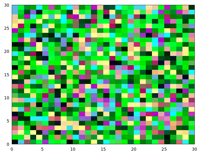
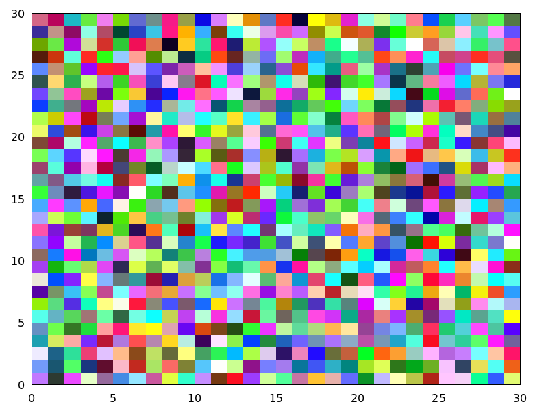
If im is a matrix of vectors of length three or an rgb picture object, they are interpreted as red, green and blue color components.
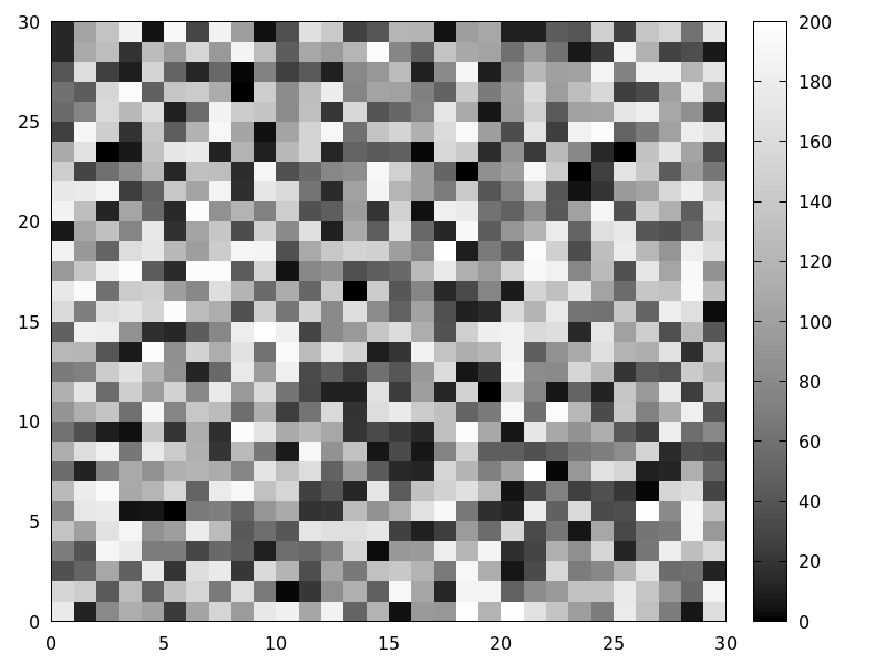
Examples:
If im is a matrix of real numbers, pixel values are interpreted according
to graphic option palette.
(%i1) im: apply(
           'matrix,
            makelist(makelist(random(200),i,1,30),i,1,30))$
(%i2) /* palette = color, default */
      draw2d(image(im,0,0,30,30))$
(%i3) draw2d(palette = gray, image(im,0,0,30,30))$
(%i4) draw2d(palette = [15,20,-4],
             colorbox=false,
             image(im,0,0,30,30))$
See also colorbox.
If im is a matrix of vectors of length three, they are interpreted as red, green and blue color components.
(%i1) im: apply(
            'matrix,
             makelist(
               makelist([random(300),
                         random(300),
                         random(300)],i,1,30),i,1,30))$
(%i2) draw2d(image(im,0,0,30,30))$
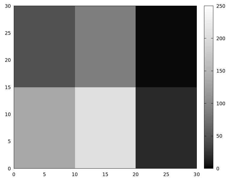
Package draw automatically loads package picture. In this
example, a level picture object is built by hand and then rendered.
(%i1) im: make_level_picture([45,87,2,134,204,16],3,2);
(%o1)       picture(level, 3, 2, {Array:  #(45 87 2 134 204 16)})
(%i2) /* default color palette */
      draw2d(image(im,0,0,30,30))$
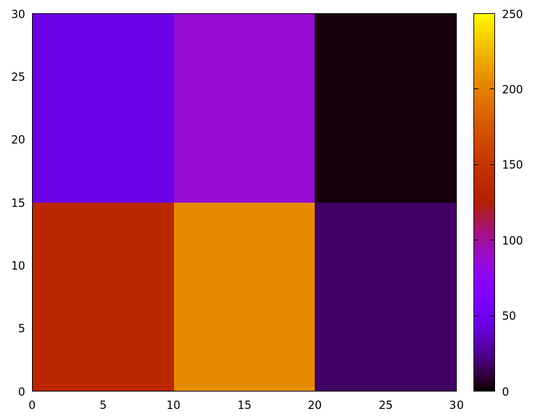
(%i3) /* gray palette */
      draw2d(palette = gray,
             image(im,0,0,30,30))$
An xpm file is read and then rendered.
(%i1) im: read_xpm("myfile.xpm")$
(%i2) draw2d(image(im,0,0,10,7))$
See also make_level_picture, make_rgb_picture and read_005fxpm.
http://www.telefonica.net/web2/biomates/maxima/gpdraw/image
contains more elaborated examples.
See also: colorbox, make_level_picture, make_rgb_picture, read_xpm.
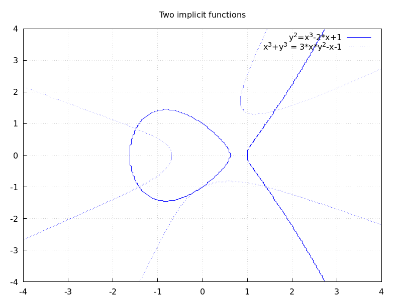
implicit (fcn, x, xmin, xmax, y, ymin, ymax) — Function
Draws implicit functions in 2D and 3D.
2D
implicit(fcn,x,xmin,xmax,y,ymin,ymax)
plots the implicit function defined by fcn, with variable x taking values
from xmin to xmax, and variable y taking values
from ymin to ymax.
This object is affected by the following graphic options: ip_grid,
ip_grid_in, line_width, line_type, key and color.
Example:
(%i1) draw2d(grid      = true,
             line_type = solid,
             key       = "y^2=x^3-2*x+1",
             implicit(y^2=x^3-2*x+1, x, -4,4, y, -4,4),
             line_type = dots,
             key       = "x^3+y^3 = 3*x*y^2-x-1",
             implicit(x^3+y^3 = 3*x*y^2-x-1, x,-4,4, y,-4,4),
             title     = "Two implicit functions" )$
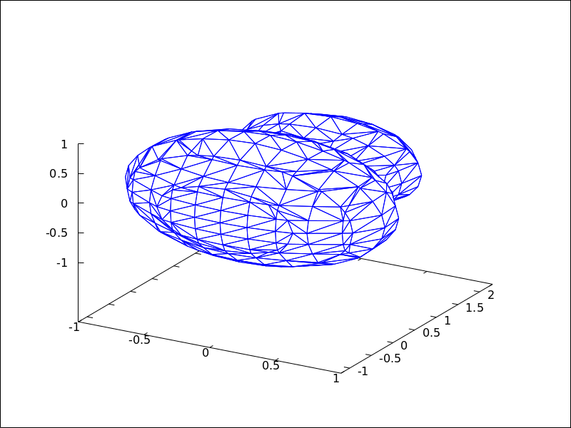
3D
implicit (fcn,x,xmin,xmax, y,ymin,ymax, z,zmin,zmax)
plots the implicit surface defined by fcn, with variable x taking values
from xmin to xmax, variable y taking values
from ymin to ymax and variable z taking values
from zmin to zmax. This object implements the marching cubes algorithm.
This object is affected by the following graphic options: x_voxel,
y_voxel, z_voxel, line_width, line_type, key,
wired_surface, enhanced3d and color.
Example:
(%i1) draw3d(
        color=blue,
        implicit((x^2+y^2+z^2-1)*(x^2+(y-1.5)^2+z^2-0.5)=0.015,
                 x,-1,1,y,-1.2,2.3,z,-1,1),
        surface_hide=true);
See also: ip_grid, ip_grid_in, line_width, line_type, key, x_voxel, y_voxel, z_voxel, wired_surface, enhanced3d.
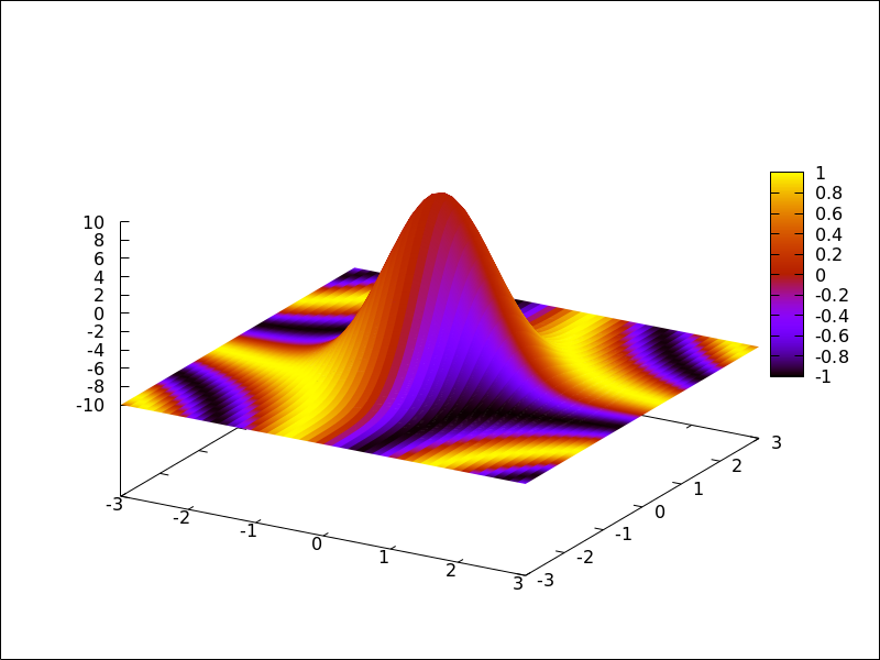
interpolate_color — Variable
Default value: false
This option is relevant only when enhanced3d is not false.
When interpolate_color is false, surfaces are colored with
homogeneous quadrangles. When true, color transitions are smoothed
by interpolation.
interpolate_color also accepts a list of two numbers, [m,n].
For positive m and n, each quadrangle or triangle is interpolated
m times and n times in the respective direction. For negative
m and n, the interpolation frequency is chosen so that there will be at least
|m| and |n| points drawn; you can consider this as a special gridding function.
Zeros, i.e. interpolate_color=[0,0], will automatically choose an
optimal number of interpolated surface points.
Also, interpolate_color=true is equivalent to interpolate_color=[0,0].
Examples:
Color interpolation with explicit functions.
(%i1) draw3d(
        enhanced3d   = sin(x*y),
        explicit(20*exp(-x^2-y^2)-10, x ,-3, 3, y, -3, 3)) $

(%i2) draw3d(
        interpolate_color = true,
        enhanced3d   = sin(x*y),
        explicit(20*exp(-x^2-y^2)-10, x ,-3, 3, y, -3, 3)) $

(%i3) draw3d(
        interpolate_color = [-10,0],
        enhanced3d   = sin(x*y),
        explicit(20*exp(-x^2-y^2)-10, x ,-3, 3, y, -3, 3)) $
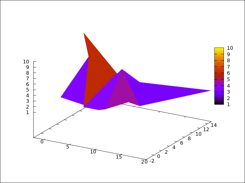
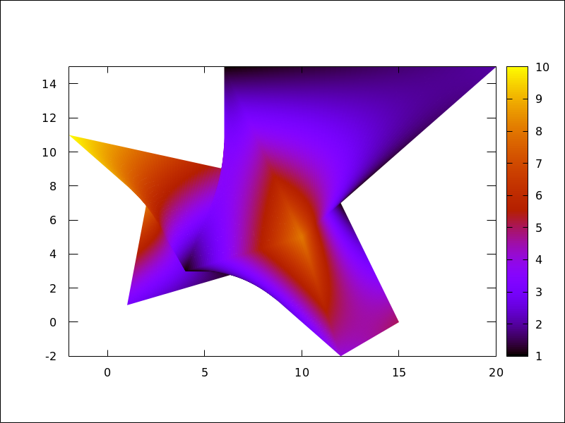
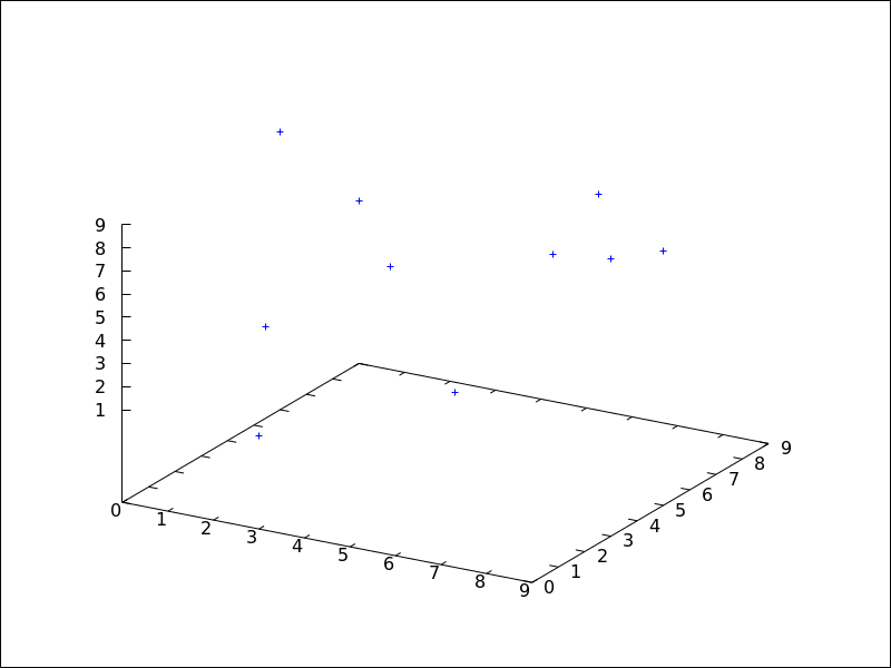
Color interpolation with the mesh graphic object.
Interpolating colors in parametric surfaces can give unexpected results.
(%i1) draw3d(
        enhanced3d = true,
        mesh([[1,1,3],   [7,3,1],[12,-2,4],[15,0,5]],
             [[2,7,8],   [4,3,1],[10,5,8], [12,7,1]],
             [[-2,11,10],[6,9,5],[6,15,1], [20,15,2]])) $
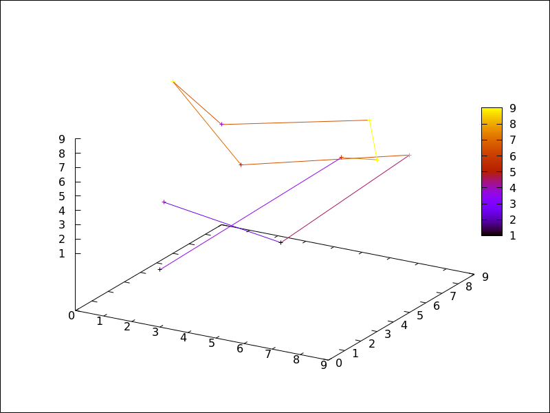
(%i2) draw3d(
        enhanced3d        = true,
        interpolate_color = true,
        mesh([[1,1,3],   [7,3,1],[12,-2,4],[15,0,5]],
             [[2,7,8],   [4,3,1],[10,5,8], [12,7,1]],
             [[-2,11,10],[6,9,5],[6,15,1], [20,15,2]])) $
(%i3) draw3d(
        enhanced3d        = true,
        interpolate_color = true,
        view=map,
        mesh([[1,1,3],   [7,3,1],[12,-2,4],[15,0,5]],
             [[2,7,8],   [4,3,1],[10,5,8], [12,7,1]],
             [[-2,11,10],[6,9,5],[6,15,1], [20,15,2]])) $
See also enhanced3d.
See also: enhanced3d.
ip_grid — Variable
Default value: [50, 50]
ip_grid sets the grid for the first sampling in implicit plots.
This option is relevant only for implicit objects.
ip_grid_in — Variable
Default value: [5, 5]
ip_grid_in sets the grid for the second sampling in implicit plots.
This option is relevant only for implicit objects.
key — Variable
Default value: "" (empty string)
key is the name of a function in the legend. If key is an
empty string, no key is assigned to the function.
This option affects the following graphic objects:
gr2d: points, polygon, rectangle,
ellipse, vector, explicit, implicit,
parametric and polar.
gr3d: points, explicit, parametric
and parametric_005fsurface.
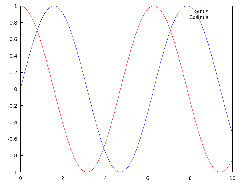
Example:
(%i1) draw2d(key   = "Sinus",
             explicit(sin(x),x,0,10),
             key   = "Cosinus",
             color = red,
             explicit(cos(x),x,0,10) )$
See also: points, polygon, rectangle, ellipse, vector, explicit, implicit, parametric, polar, parametric_surface.
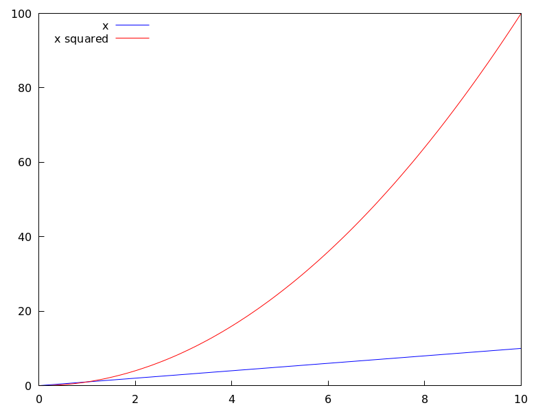
key_pos — Variable
Default value: "" (empty string)
key_pos defines at which position the legend will be drawn. If key is an
empty string, "top_right" is used.
Available position specifiers are: top_left, top_center, top_right,
center_left, center, center_right,
bottom_left, bottom_center, and bottom_right.
Since this is a global graphics option, its position in the scene description does not matter.
Example:
(%i1) draw2d(
key_pos = top_left,
key = "x",
explicit(x, x,0,10),
color= red,
key = "x squared",
explicit(x^2,x,0,10))$
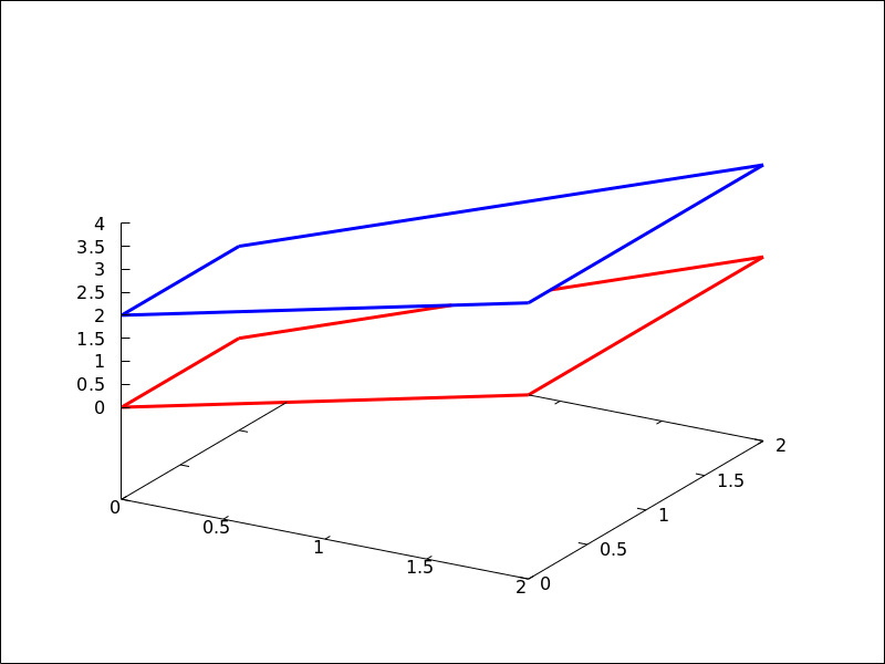
(%i3) draw3d(
key_pos = center,
key = "x",
explicit(x+y,x,0,10,y,0,10),
color= red,
key = "x squared",
explicit(x^2+y^2,x,0,10,y,0,10))$
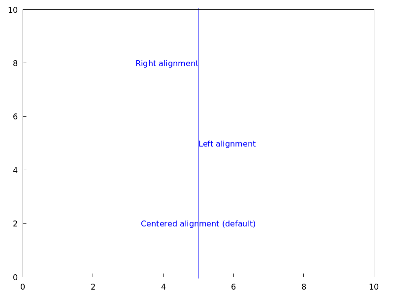
label_alignment — Variable
Default value: center
label_alignment is used to specify where to write labels with
respect to the given coordinates. Possible values are: center,
left, and right.
This option is relevant only for label objects.
Example:
(%i1) draw2d(xrange          = [0,10],
             yrange          = [0,10],
             points_joined   = true,
             points([[5,0],[5,10]]),
             color           = blue,
             label(["Centered alignment (default)",5,2]),
             label_alignment = 'left,
             label(["Left alignment",5,5]),
             label_alignment = 'right,
             label(["Right alignment",5,8]))$
See also label_orientation, and color
See also: label_orientation.
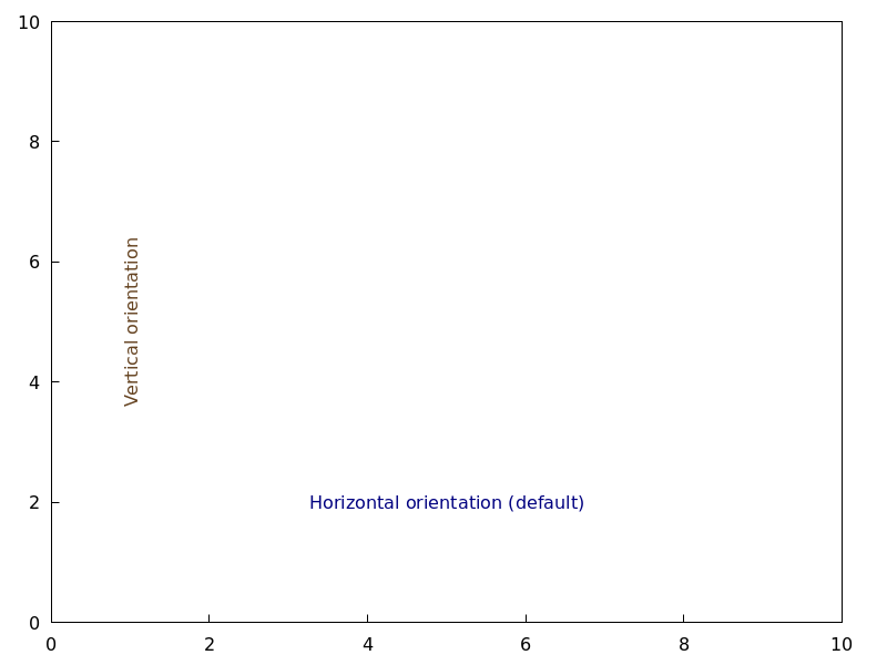
label_orientation — Variable
Default value: horizontal
label_orientation is used to specify orientation of labels.
Possible values are: horizontal, and vertical.
This option is relevant only for label objects.
Example:
In this example, a dummy point is added to get an image.
Package draw needs always data to draw an scene.
(%i1) draw2d(xrange     = [0,10],
             yrange     = [0,10],
             point_size = 0,
             points([[5,5]]),
             color      = navy,
             label(["Horizontal orientation (default)",5,2]),
             label_orientation = 'vertical,
             color             = "#654321",
             label(["Vertical orientation",1,5]))$
See also label_alignment and color
See also: label_alignment.
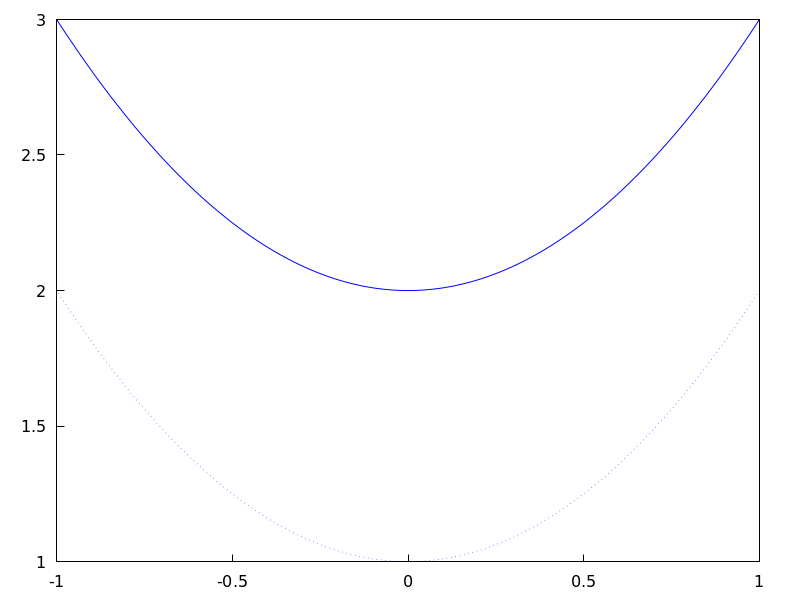
line_type — Variable
Default value: solid
line_type indicates how lines are displayed; possible values are
solid and dots, both available in all terminals, and
dashes, short_dashes, short_long_dashes, short_short_long_dashes,
and dot_dash, which are not available in png, jpg, and gif terminals.
This option affects the following graphic objects:
gr2d: points, polygon, rectangle,
ellipse, vector, explicit, implicit,
parametric and polar.
gr3d: points, explicit, parametric and parametric_005fsurface.
Example:
(%i1) draw2d(line_type = dots,
             explicit(1 + x^2,x,-1,1),
             line_type = solid, /* default */
             explicit(2 + x^2,x,-1,1))$
See also line_005fwidth.
See also: points, polygon, rectangle, ellipse, vector, explicit, implicit, parametric, polar, parametric_surface, line_width.
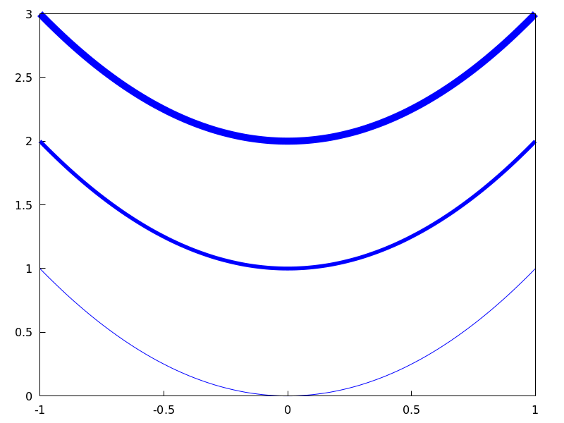
line_width — Variable
Default value: 1
line_width is the width of plotted lines.
Its value must be a positive number.
This option affects the following graphic objects:
gr2d: points, polygon, rectangle,
ellipse, vector, explicit, implicit,
parametric and polar.
gr3d: points and parametric.
Example:
(%i1) draw2d(explicit(x^2,x,-1,1), /* default width */
             line_width = 5.5,
             explicit(1 + x^2,x,-1,1),
             line_width = 10,
             explicit(2 + x^2,x,-1,1))$
See also line_005ftype.
See also: points, polygon, rectangle, ellipse, vector, explicit, implicit, parametric, polar, line_type.
logcb — Variable
Default value: false
If logcb is true, the tics in the colorbox will be drawn in the
logarithmic scale.
When enhanced3d or colorbox is false, option logcb has
no effect.
Since this is a global graphics option, its position in the scene description does not matter.
Example:
(%i1) draw3d (
        enhanced3d = true,
        color      = green,
        logcb = true,
        logz  = true,
        palette = [-15,24,-9],
        explicit(exp(x^2-y^2), x,-2,2,y,-2,2)) $
See also enhanced3d, colorbox and cbrange.
See also: logcb, enhanced3d, colorbox, cbrange.
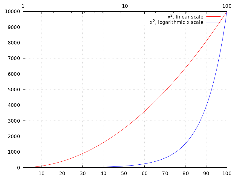
logx_secondary — Variable
Default value: false
If logx_secondary is true, the secondary x axis
will be drawn in the logarithmic scale.
This option is relevant only for 2d scenes.
Since this is a global graphics option, its position in the scene description does not matter.
Example:
(%i1) draw2d(
        grid = true,
        key="x^2, linear scale",
        color=red,
        explicit(x^2,x,1,100),
        xaxis_secondary = true,
        xtics_secondary = true,
        logx_secondary  = true,
        key = "x^2, logarithmic x scale",
        color = blue,
        explicit(x^2,x,1,100) )$
See also logx_draw, logy_draw, logy_secondary, and logz.
See also: logx_draw, logy_draw, logy_secondary, logz.
logy_secondary — Variable
Default value: false
If logy_secondary is true, the secondary y axis
will be drawn in the logarithmic scale.
This option is relevant only for 2d scenes.
Since this is a global graphics option, its position in the scene description does not matter.
Example:
(%i1) draw2d(
        grid = true,
        key="x^2, linear scale",
        color=red,
        explicit(x^2,x,1,100),
        yaxis_secondary = true,
        ytics_secondary = true,
        logy_secondary  = true,
        key = "x^2, logarithmic y scale",
        color = blue,
        explicit(x^2,x,1,100) )$
See also logx_draw, logy_draw, logx_secondary, and logz.
See also: logx_draw, logy_draw, logx_secondary, logz.
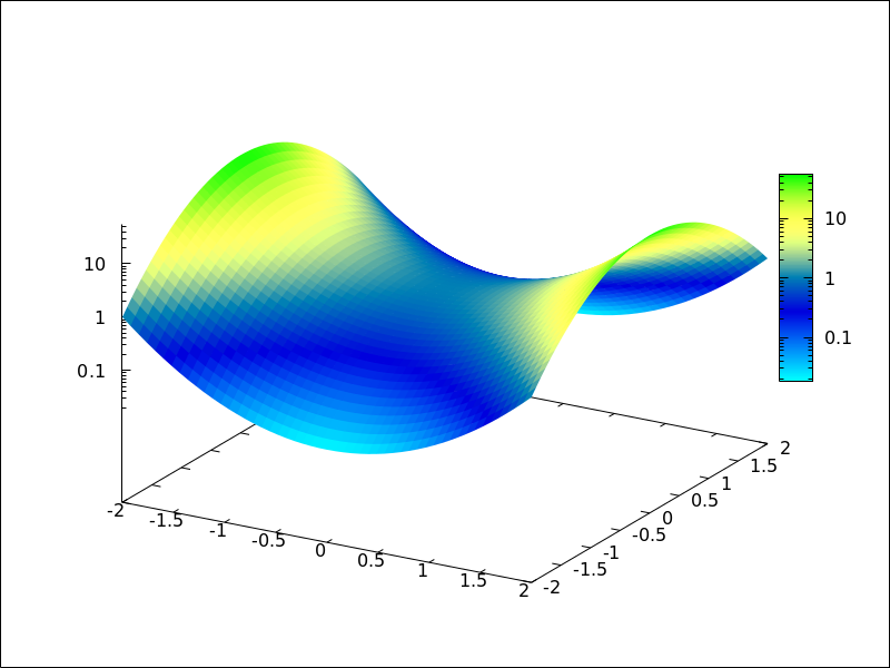
logz — Variable
Default value: false
If logz is true, the z axis will be drawn in the
logarithmic scale.
Since this is a global graphics option, its position in the scene description does not matter.
Example:
(%i1) draw3d(logz = true,
             explicit(exp(u^2+v^2),u,-2,2,v,-2,2))$
See also logx_draw and logy_005fdraw.
See also: logx_draw, logy_draw.
make_level_picture (data) — Function
Returns a levels picture object. make_level_picture (data)
builds the picture object from matrix data.
make_level_picture (data,width,height)
builds the object from a list of numbers; in this case, both the
width and the height must be given.
The returned picture object contains the following four parts:
- symbol
level - image width
- image height
- an integer array with pixel data ranging from 0 to 255. Argument data must contain only numbers ranged from 0 to 255; negative numbers are substituted by 0, and those which are greater than 255 are set to 255.
Example:
Level picture from matrix.
(%i1) make_level_picture(matrix([3,2,5],[7,-9,3000]));
(%o1)         picture(level, 3, 2, {Array:  #(3 2 5 7 0 255)})
Level picture from numeric list.
(%i1) make_level_picture([-2,0,54,%pi],2,2);
(%o1)            picture(level, 2, 2, {Array:  #(0 0 54 3)})
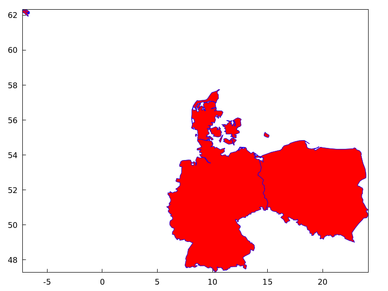
make_poly_continent (continent_name) — Function
Makes the necessary polygons to draw a colored continent or a list of countries.
Example:
(%i1) load("worldmap")$
(%i2) /* A continent */
      make_poly_continent(Africa)$
(%i3) apply(draw2d, %)$
(%i4) /* A list of countries */
      make_poly_continent([Germany,Denmark,Poland])$
(%i5) apply(draw2d, %)$
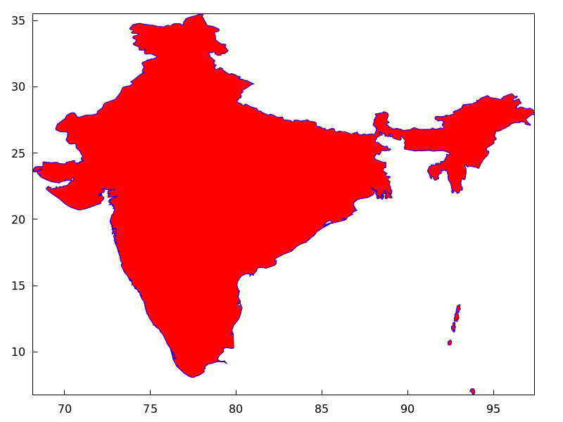
make_poly_country (country_name) — Function
Makes the necessary polygons to draw a colored country. If islands exist, one country can be defined with more than just one polygon.
Example:
(%i1) load("worldmap")$
(%i2) make_poly_country(India)$
(%i3) apply(draw2d, %)$
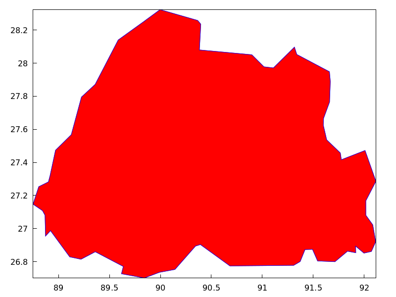
make_polygon (nlist) — Function
Returns a polygon object from boundary indices. Argument
nlist is a list of components of boundaries_array.
Example:
Bhutan is defined by boundary numbers 171, 173
and 1143, so that make_polygon([171,173,1143])
appends arrays of coordinates boundaries_array[171],
boundaries_array[173] and boundaries_array[1143] and
returns a polygon object suited to be plotted by
draw. To avoid an error message, arrays must be
compatible in the sense that any two consecutive
arrays have two coordinates in the extremes in common. In this
example, the two first components of boundaries_array[171] are
equal to the last two coordinates of boundaries_array[173], and
the two first of boundaries_array[173] are equal to the two first
of boundaries_array[1143]; in conclusion, boundary numbers
171, 173 and 1143 (in this order) are compatible and the colored
polygon can be drawn.
(%i1) load("worldmap")$
(%i2) Bhutan;
(%o2)                        [[171, 173, 1143]]
(%i3) boundaries_array[171];
(%o3) {Array:
       #(88.750549 27.14727 88.806351 27.25305 88.901367 27.282221
         88.917877 27.321039)}
(%i4) boundaries_array[173];
(%o4) {Array:
       #(91.659554 27.76511 91.6008 27.66666 91.598022 27.62499
         91.631348 27.536381 91.765533 27.45694 91.775253 27.4161
         92.007751 27.471939 92.11441 27.28583 92.015259 27.168051
         92.015533 27.08083 92.083313 27.02277 92.112183 26.920271
         92.069977 26.86194 91.997192 26.85194 91.915253 26.893881
         91.916924 26.85416 91.8358 26.863331 91.712479 26.799999
         91.542191 26.80444 91.492188 26.87472 91.418854 26.873329
         91.371353 26.800831 91.307457 26.778049 90.682457 26.77417
         90.392197 26.903601 90.344131 26.894159 90.143044 26.75333
         89.98996 26.73583 89.841919 26.70138 89.618301 26.72694
         89.636093 26.771111 89.360786 26.859989 89.22081 26.81472
         89.110237 26.829161 88.921631 26.98777 88.873016 26.95499
         88.867737 27.080549 88.843307 27.108601 88.750549
         27.14727)}
(%i5) boundaries_array[1143];
(%o5) {Array:
       #(91.659554 27.76511 91.666924 27.88888 91.65831 27.94805
         91.338028 28.05249 91.314972 28.096661 91.108856 27.971109
         91.015808 27.97777 90.896927 28.05055 90.382462 28.07972
         90.396088 28.23555 90.366074 28.257771 89.996353 28.32333
         89.83165 28.24888 89.58609 28.139999 89.35997 27.87166
         89.225517 27.795 89.125793 27.56749 88.971077 27.47361
         88.917877 27.321039)}
(%i6) Bhutan_polygon: make_polygon([171,173,1143])$
(%i7) draw2d(Bhutan_polygon)$
make_rgb_picture (redlevel, greenlevel, bluelevel) — Function
Returns an rgb-coloured picture object. All three arguments must be levels picture; with red, green and blue levels.
The returned picture object contains the following four parts:
- symbol
rgb - image width
- image height
- an integer array of length 3widthheight with pixel data ranging from 0 to 255. Each pixel is represented by three consecutive numbers (red, green, blue).
Example:
(%i1) red: make_level_picture(matrix([3,2],[7,260]));
(%o1)           picture(level, 2, 2, {Array:  #(3 2 7 255)})
(%i2) green: make_level_picture(matrix([54,23],[73,-9]));
(%o2)           picture(level, 2, 2, {Array:  #(54 23 73 0)})
(%i3) blue: make_level_picture(matrix([123,82],[45,32.5698]));
(%o3)          picture(level, 2, 2, {Array:  #(123 82 45 33)})
(%i4) make_rgb_picture(red,green,blue);
(%o4) picture(rgb, 2, 2,
              {Array:  #(3 54 123 2 23 82 7 73 45 255 0 33)})
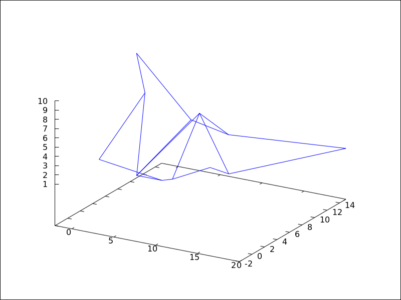
mesh (row_1, row_2, …) — Function
Draws a quadrangular mesh in 3D.
3D
Argument row_i is a list of n 3D points of the form
[[x_i1,y_i1,z_i1], ...,[x_in,y_in,z_in]], and all rows are
of equal length. All these points define an arbitrary surface in 3D and
in some sense it’s a generalization of the elevation_grid object.
This object is affected by the following graphic options: line_type,
line_width, color, key, wired_surface, enhanced3d and transform.
Examples:
A simple example.
(%i1) draw3d(
         mesh([[1,1,3],   [7,3,1],[12,-2,4],[15,0,5]],
              [[2,7,8],   [4,3,1],[10,5,8], [12,7,1]],
              [[-2,11,10],[6,9,5],[6,15,1], [20,15,2]])) $
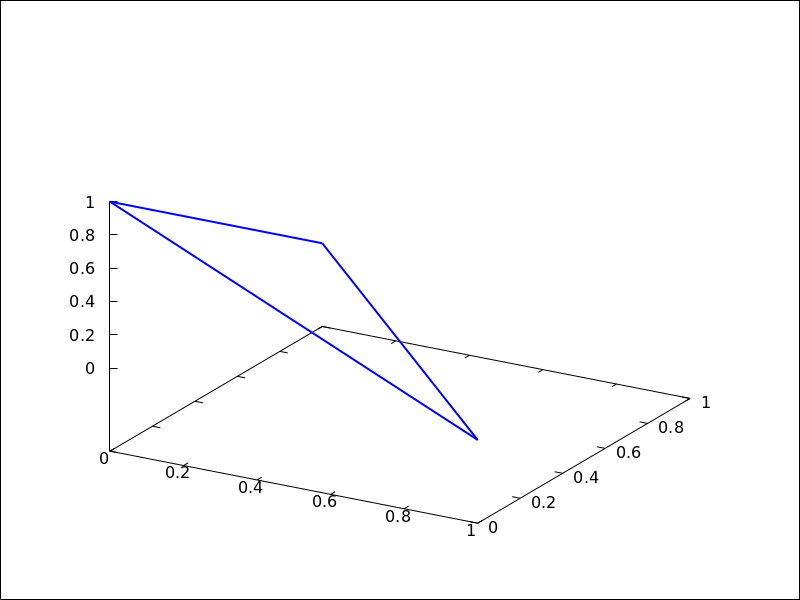
Plotting a triangle in 3D.
(%i1) draw3d(
        line_width = 2,
        mesh([[1,0,0],[0,1,0]],
             [[0,0,1],[0,0,1]])) $
Two quadrilaterals.
(%i1) draw3d(
        surface_hide = true,
        line_width   = 3,
        color = red,
        mesh([[0,0,0], [0,1,0]],
             [[2,0,2], [2,2,2]]),
        color = blue,
        mesh([[0,0,2], [0,1,2]],
             [[2,0,4], [2,2,4]])) $
See also: line_type, line_width, color, key, wired_surface, enhanced3d, transform.
multiplot_mode (term) — Function
This function enables Maxima to work in one-window multiplot mode with terminal
term; accepted arguments for this function are screen,
wxt, aquaterm, windows and none.
When multiplot mode is enabled, each call to draw sends a new plot to the
same window, without erasing the previous ones. To disable the multiplot mode,
write multiplot_mode(none).
When multiplot mode is enabled, global option terminal is blocked and you
have to disable this working mode before changing to another terminal.
On Windows this feature requires Gnuplot 5.0 or newer.
Note, that just plotting multiple expressions into the same plot doesn’t require
multiplot: It can be done by just issuing multiple explicit or similar
commands in a row.
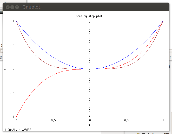
Example:
(%i1) set_draw_defaults(
         xrange = [-1,1],
         yrange = [-1,1],
         grid   = true,
         title  = "Step by step plot" )$
(%i2) multiplot_mode(screen)$
(%i3) draw2d(color=blue,  explicit(x^2,x,-1,1))$
(%i4) draw2d(color=red,   explicit(x^3,x,-1,1))$
(%i5) draw2d(color=brown, explicit(x^4,x,-1,1))$
(%i6) multiplot_mode(none)$
See also: explicit.
negative_picture (pic) — Function
Returns the negative of a (level or rgb) picture.
numbered_boundaries (nlist) — Function
Draws a list of polygonal segments (boundaries), labeled by
its numbers (boundaries_array coordinates). This is of great
help when building new geographical entities.
Example:
Map of Europe labeling borders with their component number in
boundaries_array.
(%i1) load("worldmap")$
(%i2) european_borders:
           region_boundaries(-31.81,74.92,49.84,32.06)$
(%i3) numbered_boundaries(european_borders)$
parametric (xfun, yfun, par, parmin, parmax) — Function
Draws parametric functions in 2D and 3D.
This object is affected by the following graphic options: nticks,
line_width, line_type, key, color and enhanced3d.
2D
The command parametric(xfun, yfun, par, parmin, parmax) plots the parametric function [xfun, yfun],
with parameter par taking values from parmin to parmax.
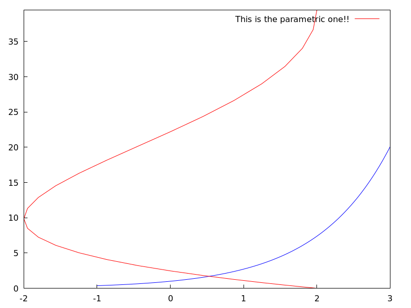
Example:
(%i1) draw2d(explicit(exp(x),x,-1,3),
             color = red,
             key   = "This is the parametric one!!",
             parametric(2*cos(rrr),rrr^2,rrr,0,2*%pi))$
3D
parametric(xfun, yfun, zfun, par, parmin, parmax) plots the parametric curve [xfun, yfun, zfun], with parameter par taking values from parmin to
parmax.
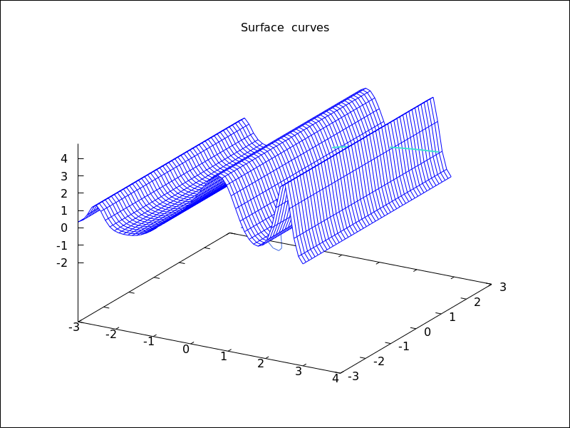
Example:
(%i1) draw3d(explicit(exp(sin(x)+cos(x^2)),x,-3,3,y,-3,3),
             color = royalblue,
             parametric(cos(5*u)^2,sin(7*u),u-2,u,0,2),
             color      = turquoise,
             line_width = 2,
             parametric(t^2,sin(t),2+t,t,0,2),
             surface_hide = true,
             title = "Surface & curves" )$
See also: nticks, line_width, line_type, key, color, enhanced3d.
parametric_surface (xfun, yfun, zfun, par1, par1min, par1max, par2, par2min, par2max) — Function
Draws parametric surfaces in 3D.
3D
The command parametric_surface(xfun, yfun, zfun, par1, par1min, par1max, par2, par2min, par2max) plots the parametric surface [xfun, yfun, zfun], with parameter par1 taking values from par1min to
par1max and parameter par2 taking values from par2min to
par2max.
This object is affected by the following graphic options: draw_realpart, xu_grid,
yv_grid, line_type, line_width, key, wired_surface, enhanced3d
and color.
Example:
(%i1) draw3d(title          = "Sea shell",
             xu_grid        = 100,
             yv_grid        = 25,
             view           = [100,20],
             surface_hide   = true,
             parametric_surface(0.5*u*cos(u)*(cos(v)+1),
                           0.5*u*sin(u)*(cos(v)+1),
                           u*sin(v) - ((u+3)/8*%pi)^2 - 20,
                           u, 0, 13*%pi, v, -%pi, %pi) )$
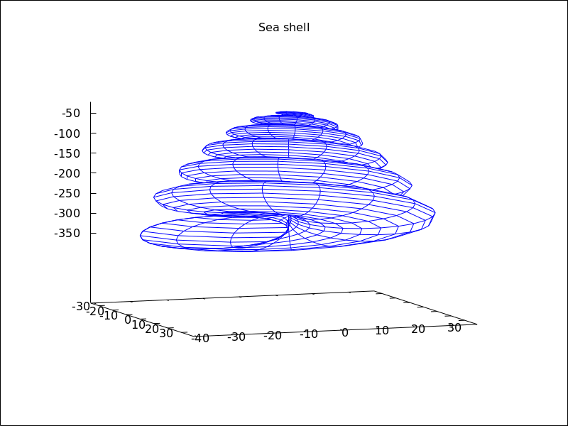
See also: draw_realpart, xu_grid, yv_grid, line_type, line_width, key, wired_surface, enhanced3d.
picture_equalp (x, y) — Function
Returns true in case of equal pictures, and false otherwise.
picturep (x) — Function
Returns true if the argument is a well formed image,
and false otherwise.
point_size — Variable
Default value: 1
point_size sets the size for plotted points. It must be a
non negative number.
This option has no effect when graphic option point_type is
set to dot.
This option affects the following graphic objects:
gr2d: points.
gr3d: points.
Example:
(%i1) draw2d(points(makelist([random(20),random(50)],k,1,10)),
        point_size = 5,
        points(makelist(k,k,1,20),makelist(random(30),k,1,20)))$
See also: points.
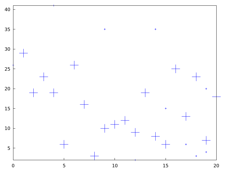
points ([[x1, y1], [x2, y2], …]) — Function
Draws points in 2D and 3D.
This object is affected by the following graphic options: point_size,
point_type, points_joined, line_width, key,
line_type and color. In 3D mode, it is also affected by enhanced3d
2D
points ([[x1,y1], [x2,y2],...]) or
points ([x1,x2,...], [y1,y2,...])
plots points [x1,y1], [x2,y2], etc. If abscissas
are not given, they are set to consecutive positive integers, so that
points ([y1,y2,...]) draws points [1,y1], [2,y2], etc.
If matrix is a two-column or two-row matrix, points (matrix)
draws the associated points. If matrix is an one-column or one-row matrix,
abscissas are assigned automatically.
If 1d_y_array is a 1D lisp array of numbers, points (1d_y_array) plots them
setting abscissas to consecutive positive integers. points (1d_x_array, 1d_y_array)
plots points with their coordinates taken from the two arrays passed as arguments. If
2d_xy_array is a 2D array with two columns, or with two rows, points (2d_xy_array)
plots the corresponding points on the plane.
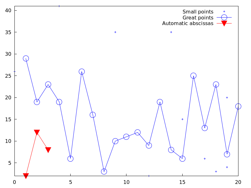
Examples:
Two types of arguments for points, a list of pairs and two lists
of separate coordinates.
(%i1) draw2d(
        key = "Small points",
        points(makelist([random(20),random(50)],k,1,10)),
        point_type    = circle,
        point_size    = 3,
        points_joined = true,
        key           = "Great points",
        points(makelist(k,k,1,20),makelist(random(30),k,1,20)),
        point_type    = filled_down_triangle,
        key           = "Automatic abscissas",
        color         = red,
        points([2,12,8]))$
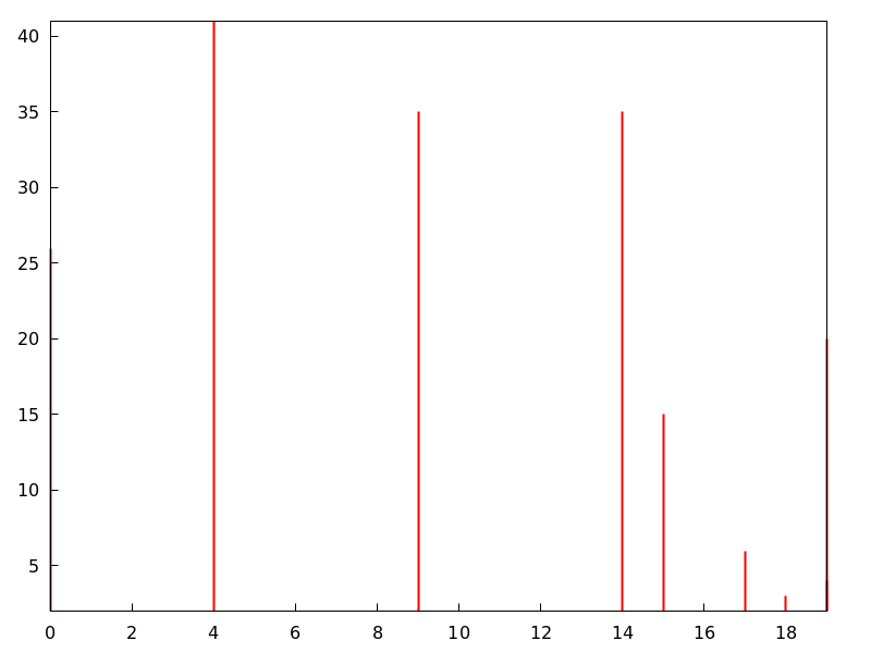
Drawing impulses.
(%i1) draw2d(
        points_joined = impulses,
        line_width    = 2,
        color         = red,
        points(makelist([random(20),random(50)],k,1,10)))$
Array with ordinates.
(%i1) a: make_array (flonum, 100) $
(%i2) for i:0 thru 99 do a[i]: random(1.0) $
(%i3) draw2d(points(a)) $
Two arrays with separate coordinates.
(%i1) x: make_array (flonum, 100) $
(%i2) y: make_array (fixnum, 100) $
(%i3) for i:0 thru 99 do (
        x[i]: float(i/100),
        y[i]: random(10) ) $
(%i4) draw2d(points(x, y)) $
A two-column 2D array.
(%i1) xy: make_array(flonum, 100, 2) $
(%i2) for i:0 thru 99 do (
        xy[i, 0]: float(i/100),
        xy[i, 1]: random(10) ) $
(%i3) draw2d(points(xy)) $

Drawing an array filled with function read_array.
(%i1) a: make_array(flonum,100) $
(%i2) read_array (file_search ("pidigits.data"), a) $
(%i3) draw2d(points(a)) $
3D
points([[x1, y1, z1], [x2, y2, z2], ...]) or points([x1, x2, ...], [y1, y2, ...], [z1, z2,...]) plots points [x1, y1, z1],
[x2, y2, z2], etc. If matrix is a three-column
or three-row matrix, points (matrix) draws the associated points.
When arguments are lisp arrays, points (1d_x_array, 1d_y_array, 1d_z_array)
takes coordinates from the three 1D arrays. If 2d_xyz_array is a 2D array with three columns,
or with three rows, points (2d_xyz_array) plots the corresponding points.
Examples:
One tridimensional sample,
(%i1) load ("numericalio")$
(%i2) s2 : read_matrix (file_search ("wind.data"))$
(%i3) draw3d(title = "Daily average wind speeds",
             point_size = 2,
             points(args(submatrix (s2, 4, 5))) )$
Two tridimensional samples,
(%i1) load ("numericalio")$
(%i2) s2 : read_matrix (file_search ("wind.data"))$
(%i3) draw3d(
         title = "Daily average wind speeds. Two data sets",
         point_size = 2,
         key        = "Sample from stations 1, 2 and 3",
         points(args(submatrix (s2, 4, 5))),
         point_type = 4,
         key        = "Sample from stations 1, 4 and 5",
         points(args(submatrix (s2, 2, 3))) )$
Unidimensional arrays,
(%i1) x: make_array (fixnum, 10) $
(%i2) y: make_array (fixnum, 10) $
(%i3) z: make_array (fixnum, 10) $
(%i4) for i:0 thru 9 do (
        x[i]: random(10),
        y[i]: random(10),
        z[i]: random(10) ) $
(%i5) draw3d(points(x,y,z)) $
Bidimensional colored array,
(%i1) xyz: make_array(fixnum, 10, 3) $
(%i2) for i:0 thru 9 do (
        xyz[i, 0]: random(10),
        xyz[i, 1]: random(10),
        xyz[i, 2]: random(10) ) $
(%i3) draw3d(
         enhanced3d = true,
         points_joined = true,
         points(xyz)) $
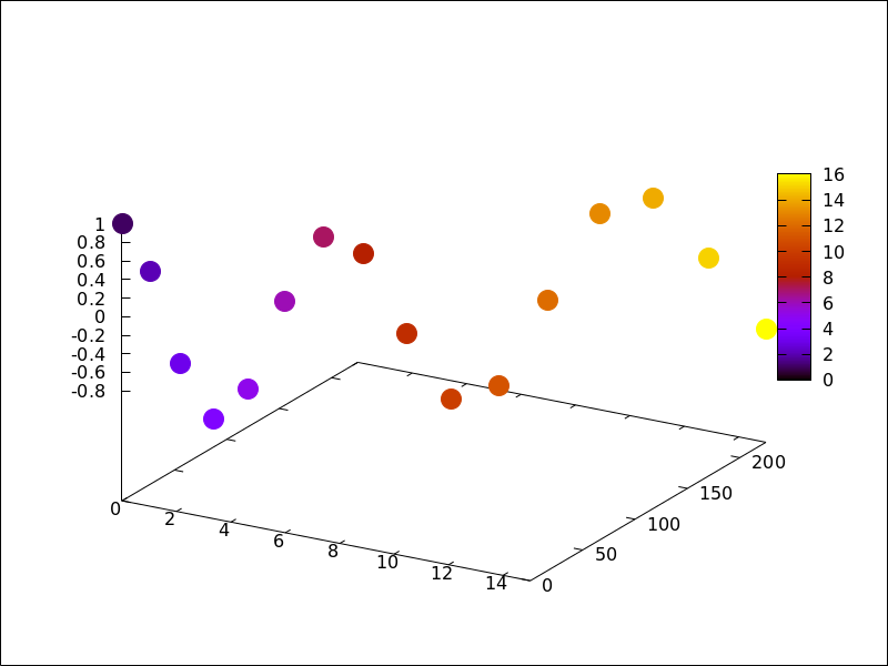
Color numbers explicitly specified by the user.
(%i1) pts: makelist([t,t^2,cos(t)], t, 0, 15)$
(%i2) col_num: makelist(k, k, 1, length(pts))$
(%i3) draw3d(
        enhanced3d = ['part(col_num,k),k],
        point_size = 3,
        point_type = filled_circle,
        points(pts))$
See also: point_size, point_type, points_joined, line_width, key, line_type, enhanced3d.
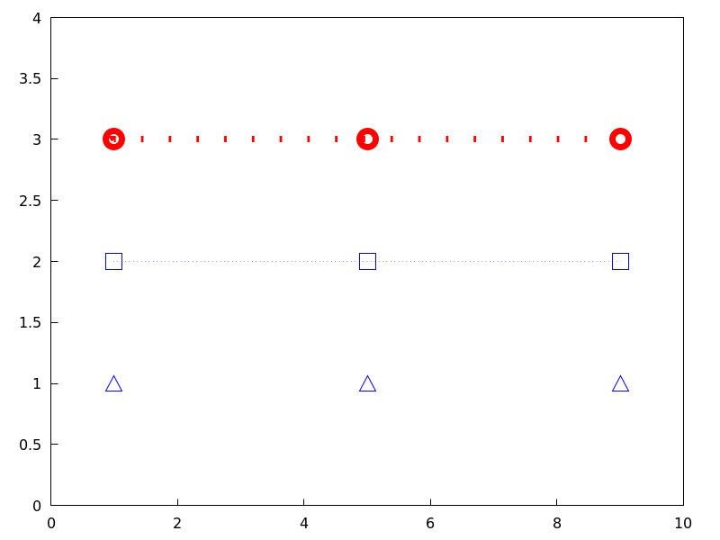
points_joined — Variable
Default value: false
When points_joined is true, points are joined by lines; when false,
isolated points are drawn. A third possible value for this graphic option is
impulses; in such case, vertical segments are drawn from points to the x-axis (2D)
or to the xy-plane (3D).
This option affects the following graphic objects:
gr2d: points.
gr3d: points.
Example:
(%i1) draw2d(xrange        = [0,10],
             yrange        = [0,4],
             point_size    = 3,
             point_type    = up_triangle,
             color         = blue,
             points([[1,1],[5,1],[9,1]]),
             points_joined = true,
             point_type    = square,
             line_type     = dots,
             points([[1,2],[5,2],[9,2]]),
             point_type    = circle,
             color         = red,
             line_width    = 7,
             points([[1,3],[5,3],[9,3]]) )$
See also: points.
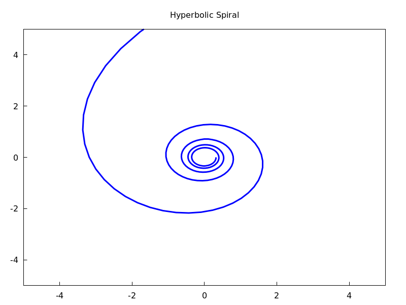
polar (radius, ang, minang, maxang) — Function
Draws 2D functions defined in polar coordinates.
2D
polar (radius,ang,minang,maxang) plots function
radius(ang) defined in polar coordinates, with variable
ang taking values from
minang to maxang.
This object is affected by the following graphic options: nticks,
line_width, line_type, key and color.
Example:
(%i1) draw2d(user_preamble = "set grid polar",
             nticks        = 200,
             xrange        = [-5,5],
             yrange        = [-5,5],
             color         = blue,
             line_width    = 3,
             title         = "Hyperbolic Spiral",
             polar(10/theta,theta,1,10*%pi) )$
See also: nticks, line_width, line_type, key.
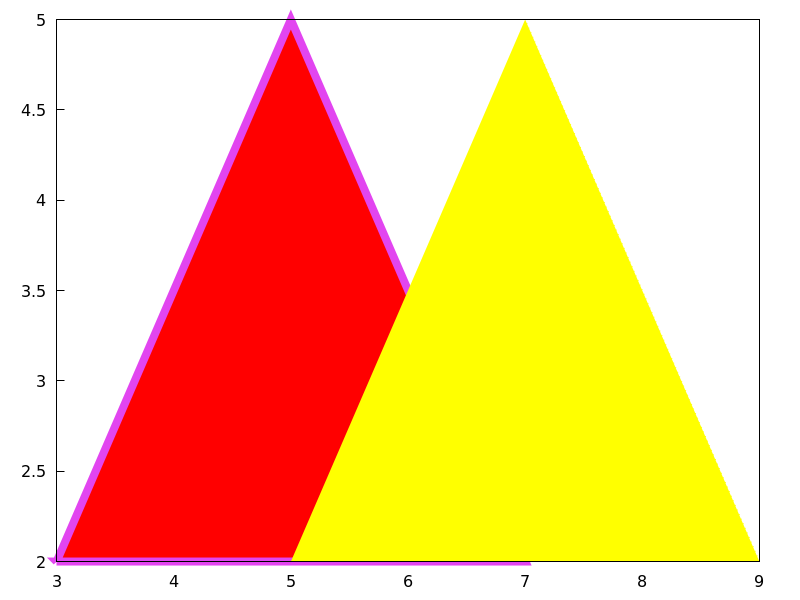
polygon ([[x1, y1], [x2, y2], …]) — Function
Draws polygons in 2D.
2D
The commands polygon([[x1, y1], [x2, y2], ...])
or polygon([x1, x2, ...], [y1, y2, ...]) plot on
the plane a polygon with vertices [x1, y1], [x2, y2], etc.
This object is affected by the following graphic options: transparent,
fill_color, fill_density, border, line_width, key,
line_type and color.
Example:
(%i1) draw2d(color      = "#e245f0",
             line_width = 8,
             polygon([[3,2],[7,2],[5,5]]),
             border      = false,
             fill_color  = yellow,
             polygon([[5,2],[9,2],[7,5]]) )$
See also: transparent, fill_color, fill_density, border, line_width, key, line_type.
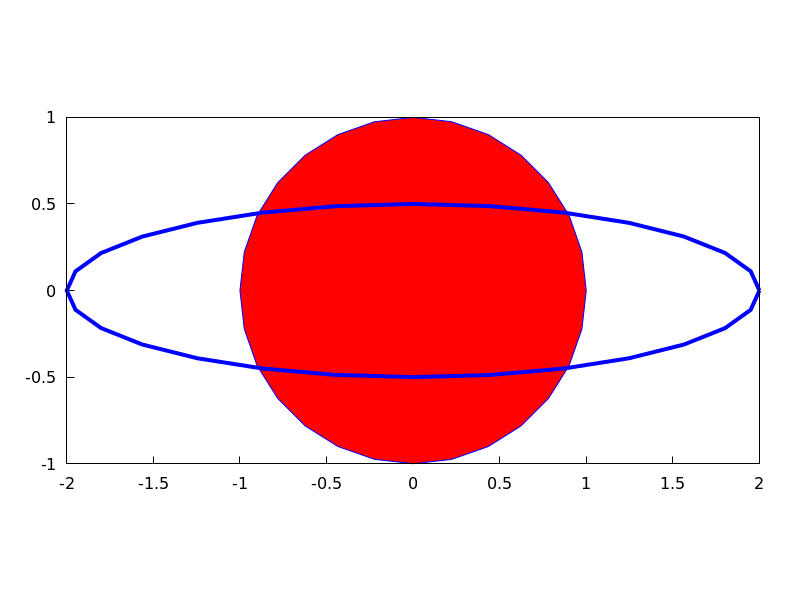
proportional_axes — Variable
Default value: none
When proportional_axes is equal to xy or xyz,
the aspect ratio of the axis units will be set to 1:1 resulting in a 2D or 3D
scene that will be drawn with axes proportional to their relative lengths.
Since this is a global graphics option, its position in the scene description does not matter.
This option works with Gnuplot version 4.2.6 or greater.
Examples:
Single 2D plot.
(%i1) draw2d(
        ellipse(0,0,1,1,0,360),
        transparent=true,
        color = blue,
        line_width = 4,
        ellipse(0,0,2,1/2,0,360),
        proportional_axes = 'xy) $
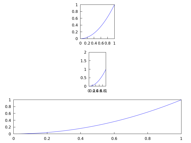
Multiplot.
(%i1) draw(
        terminal = wxt,
        gr2d(proportional_axes = 'xy,
             explicit(x^2,x,0,1)),
        gr2d(explicit(x^2,x,0,1),
             xrange = [0,1],
             yrange = [0,2],
             proportional_axes='xy),
        gr2d(explicit(x^2,x,0,1)))$
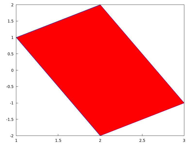
quadrilateral (point_1, point_2, point_3, point_4) — Function
Draws a quadrilateral.
2D
quadrilateral([x1, y1], [x2, y2], [x3, y3], [x4, y4]) draws a quadrilateral with vertices
[x1, y1], [x2, y2],
[x3, y3], and [x4, y4].
This object is affected by the following graphic options:
transparent, fill_color, border, line_width,
key, xaxis_secondary, yaxis_secondary, line_type,
transform and color.
Example:
(%i1) draw2d(
        quadrilateral([1,1],[2,2],[3,-1],[2,-2]))$
3D
quadrilateral([x1, y1, z1], [x2, y2, z2], [x3, y3, z3], [x4, y4, z4])
draws a quadrilateral with vertices [x1, y1, z1],
[x2, y2, z2], [x3, y3, z3],
and [x4, y4, z4].
This object is affected by the following graphic options: line_type,
line_width, color, key, enhanced3d and
transform.
See also: transparent, fill_color, border, line_width, key, xaxis_secondary, yaxis_secondary, line_type, color, enhanced3d, transform.
read_xpm (xpm_file) — Function
Reads a file in xpm and returns a picture object.
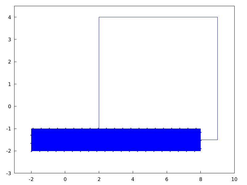
rectangle ([x1, y1], [x2, y2]) — Function
Draws rectangles in 2D.
2D
rectangle ([x1,y1], [x2,y2]) draws a rectangle with opposite vertices
[x1,y1] and [x2,y2].
This object is affected by the following graphic options: transparent,
fill_color, border, line_width, key,
line_type and color.
Example:
(%i1) draw2d(fill_color  = red,
             line_width  = 6,
             line_type   = dots,
             transparent = false,
             fill_color  = blue,
             rectangle([-2,-2],[8,-1]), /* opposite vertices */
             transparent = true,
             line_type   = solid,
             line_width  = 1,
             rectangle([9,4],[2,-1.5]),
             xrange      = [-3,10],
             yrange      = [-3,4.5] )$
See also: transparent, fill_color, border, line_width, key, line_type.
region (expr, var1, minval1, maxval1, var2, minval2, maxval2) — Function
Plots a region on the plane defined by inequalities.
2D
expr is an expression formed by inequalities and boolean operators
and, or, and not. The region is bounded by the rectangle
defined by $[minval1, maxval1]$ and $[minval2, maxval2]$.
This object is affected by the following graphic options: fill_color, fill_density,
key, x_voxel and y_005fvoxel.
Example:
(%i1) draw2d(
        x_voxel = 30,
        y_voxel = 30,
        region(x^2+y^2<1 and x^2+y^2 > 1/2,
               x, -1.5, 1.5, y, -1.5, 1.5));
See also: not, fill_color, fill_density, key, x_voxel, y_voxel.
region_boundaries (x1, y1, x2, y2) — Function
Detects polygonal segments of global variable boundaries_array
fully contained in the rectangle with vertices (x1,y1) -upper left-
and (x2,y2) -bottom right-.
Example:
Returns segment numbers for plotting southern Italy.
(%i1) load("worldmap")$
(%i2) region_boundaries(10.4,41.5,20.7,35.4);
(%o2)                [1846, 1863, 1864, 1881, 1888, 1894]
(%i3) draw2d(geomap(%))$
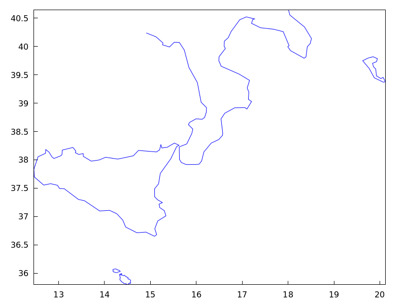
region_boundaries_plus (x1, y1, x2, y2) — Function
Detects polygonal segments of global variable boundaries_array
containing at least one vertex in the rectangle defined by vertices (x1,y1)
-upper left- and (x2,y2) -bottom right-.
Example:
(%i1) load("worldmap")$
(%i2) region_boundaries_plus(10.4,41.5,20.7,35.4);
(%o2) [1060, 1062, 1076, 1835, 1839, 1844, 1846, 1858,
       1861, 1863, 1864, 1871, 1881, 1888, 1894, 1897]
(%i3) draw2d(geomap(%))$
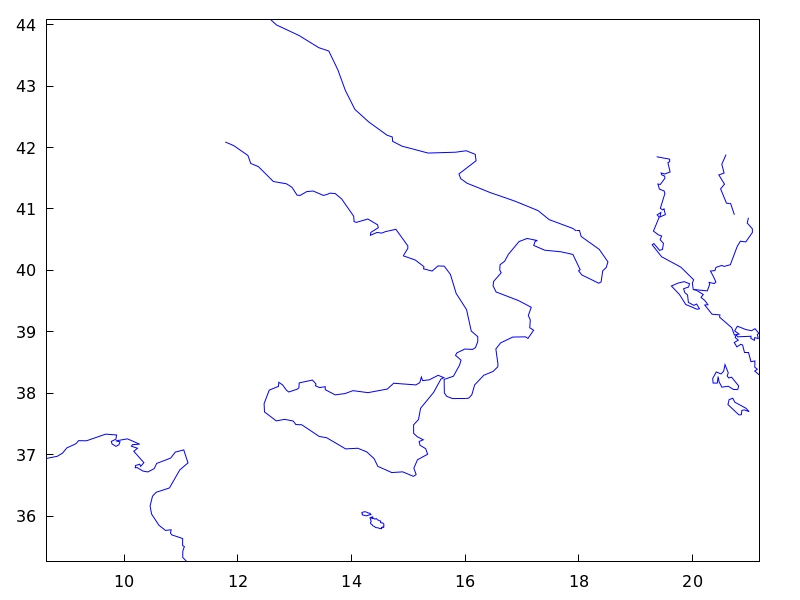
rgb2level (pic) — Function
Transforms an rgb picture into a level one by averaging the red, green and blue channels.
set_draw_defaults (graphic option, …, graphic object, …) — Function
Sets user graphics options. This function is useful for plotting a sequence of graphics with common graphics options. Calling this function without arguments removes user defaults.
Example:
(%i1) set_draw_defaults(
         xrange = [-10,10],
         yrange = [-2, 2],
         color  = blue,
         grid   = true)$
(%i2) /* plot with user defaults */
      draw2d(explicit(((1+x)**2/(1+x*x))-1,x,-10,10))$
(%i3) set_draw_defaults()$
(%i4) /* plot with standard defaults */
      draw2d(explicit(((1+x)**2/(1+x*x))-1,x,-10,10))$
spherical (radius, azi, minazi, maxazi, zen, minzen, maxzen) — Function
Draws 3D functions defined in spherical coordinates.
3D
spherical(radius, azi, minazi, maxazi, zen, minzen, maxzen) plots the function radius(azi, zen) defined in spherical coordinates, with azimuth azi taking
values from minazi to maxazi and zenith zen taking values
from minzen to maxzen.
This object is affected by the following graphic options: xu_grid,
yv_grid, line_type, key, wired_surface, enhanced3d and color.
Example:
(%i1) draw3d(spherical(1,a,0,2*%pi,z,0,%pi))$
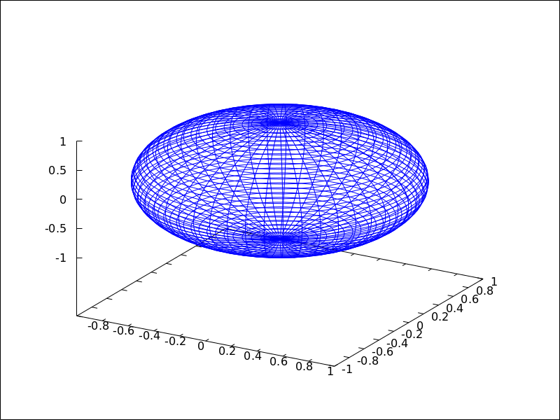
See also: xu_grid, yv_grid, line_type, key, wired_surface, enhanced3d.
surface_hide — Variable
Default value: false
If surface_hide is true, hidden parts are not plotted in 3d surfaces.
Since this is a global graphics option, its position in the scene description does not matter.
Example:
(%i1) draw(columns=2,
           gr3d(explicit(exp(sin(x)+cos(x^2)),x,-3,3,y,-3,3)),
           gr3d(surface_hide = true,
                explicit(exp(sin(x)+cos(x^2)),x,-3,3,y,-3,3)) )$
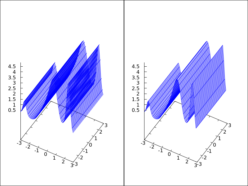
take_channel (im, color) — Function
If argument color is red, green or blue,
function take_channel returns the corresponding color channel of
picture im.
Example:
(%i1) red: make_level_picture(matrix([3,2],[7,260]));
(%o1)           picture(level, 2, 2, {Array:  #(3 2 7 255)})
(%i2) green: make_level_picture(matrix([54,23],[73,-9]));
(%o2)           picture(level, 2, 2, {Array:  #(54 23 73 0)})
(%i3) blue: make_level_picture(matrix([123,82],[45,32.5698]));
(%o3)          picture(level, 2, 2, {Array:  #(123 82 45 33)})
(%i4) make_rgb_picture(red,green,blue);
(%o4) picture(rgb, 2, 2,
              {Array:  #(3 54 123 2 23 82 7 73 45 255 0 33)})
(%i5) take_channel(%,'green);  /* simple quote!!! */
(%o5)           picture(level, 2, 2, {Array:  #(54 23 73 0)})
terminal — Variable
Default value: screen
Selects the terminal to be used by Gnuplot; possible values are:
screen (default), png, pngcairo, jpg, gif,
cairolatex_pdf, cairolatex_pdf_standalone,
eps, eps_color, epslatex, epslatex_standalone,
svg, canvas, dumb, dumb_file, pdf, pdfcairo,
wxt, animated_gif, multipage_pdfcairo, multipage_pdf,
multipage_eps, multipage_eps_color, tikz, tikz_standalone
and aquaterm.
Terminals screen, wxt, windows and aquaterm can
be also defined as a list
with two elements: the name of the terminal itself and a non negative integer number.
In this form, multiple windows can be opened at the same time, each with its
corresponding number. This feature does not work in Windows platforms.
Since this is a global graphics option, its position in the scene description
does not matter. It can be also used as an argument of function draw.
N.B. pdfcairo requires Gnuplot 4.3 or newer.
pdf requires Gnuplot to be compiled with the option --enable-pdf and libpdf must
be installed. The pdf library is available from: http://www.pdflib.com/en/download/pdflib-family/pdflib-lite/
Examples:
(%i1) /* screen terminal (default) */
      draw2d(explicit(x^2,x,-1,1))$
(%i2) /* png file */
      draw2d(terminal  = 'png,
             explicit(x^2,x,-1,1))$
(%i3) /* jpg file */
      draw2d(terminal   = 'jpg,
             dimensions = [300,300],
             explicit(x^2,x,-1,1))$
(%i4) /* eps file */
      draw2d(file_name = "myfile",
             explicit(x^2,x,-1,1),
             terminal  = 'eps)$
(%i5) /* pdf file */
      draw2d(file_name = "mypdf",
             dimensions = 100*[12.0,8.0],
             explicit(x^2,x,-1,1),
             terminal  = 'pdf)$
(%i6) /* wxwidgets window */
      draw2d(explicit(x^2,x,-1,1),
             terminal  = 'wxt)$
(%i7) /* tikz file */
      draw2d(explicit(x^2,x,-1,1),
             file_name = "mytikz",
             dimensions = [8,8], /* in cms */
             terminal = 'tikz)$
Multiple windows.
(%i1) draw2d(explicit(x^5,x,-2,2), terminal=[screen, 3])$
(%i2) draw2d(explicit(x^2,x,-2,2), terminal=[screen, 0])$
An animated gif file.
(%i1) draw(
        delay     = 100,
        file_name = "zzz",
        terminal  = 'animated_gif,
        gr2d(explicit(x^2,x,-1,1)),
        gr2d(explicit(x^3,x,-1,1)),
        gr2d(explicit(x^4,x,-1,1)));
End of animation sequence
(%o1)          [gr2d(explicit), gr2d(explicit), gr2d(explicit)]
Option delay is only active in animated gif’s; it is ignored in
any other case.
Multipage output in eps format.
(%i1) draw(
        file_name = "parabol",
        terminal  = multipage_eps,
        dimensions = 100*[10,10],
        gr2d(explicit(x^2,x,-1,1)),
        gr3d(explicit(x^2+y^2,x,-1,1,y,-1,1))) $
See also file_name, dimensions_draw and delay.
See also: file_name, dimensions_draw, delay.
transform — Variable
Default value: none
If transform is none, the space is not transformed and
graphic objects are drawn as defined. When a space transformation is
desired, a list must be assigned to option transform. In case of
a 2D scene, the list takes the form [f1(x,y), f2(x,y), x, y].
In case of a 3D scene, the list is of the form
[f1(x,y,z), f2(x,y,z), f3(x,y,z), x, y, z].
The names of the variables defined in the lists may be different to those used in the definitions of the graphic objects.
Examples:
Rotation in 2D.
(%i1) th : %pi / 4$
(%i2) draw2d(
        color = "#e245f0",
        proportional_axes = 'xy,
        line_width = 8,
        triangle([3,2],[7,2],[5,5]),
        border     = false,
        fill_color = yellow,
        transform  = [cos(th)*x - sin(th)*y,
                      sin(th)*x + cos(th)*y, x, y],
        triangle([3,2],[7,2],[5,5]) )$
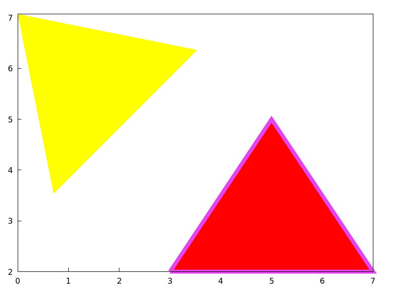
Translation in 3D.
(%i1) draw3d(
        color     = "#a02c00",
        explicit(20*exp(-x^2-y^2)-10,x,-3,3,y,-3,3),
        transform = [x+10,y+10,z+10,x,y,z],
        color     = blue,
        explicit(20*exp(-x^2-y^2)-10,x,-3,3,y,-3,3) )$
transparent — Variable
Default value: false
If transparent is false, interior regions of polygons are
filled according to fill_color.
This option affects the following graphic objects:
gr2d: polygon, rectangle and ellipse.
Example:
(%i1) draw2d(polygon([[3,2],[7,2],[5,5]]),
             transparent = true,
             color       = blue,
             polygon([[5,2],[9,2],[7,5]]) )$
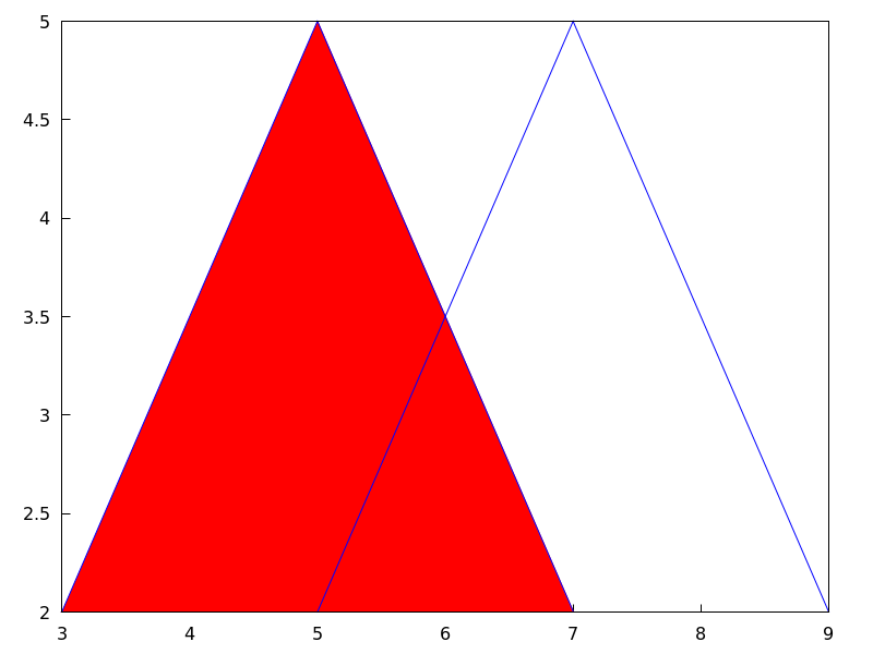
See also: polygon, rectangle, ellipse.
triangle (point_1, point_2, point_3) — Function
Draws a triangle.
2D
triangle ([x1,y1], [x2,y2], [x3,y3]) draws a triangle with vertices [x1,y1], [x2,y2],
and [x3,y3].
This object is affected by the following graphic options:
transparent, fill_color, border, line_width,
key, xaxis_secondary, yaxis_secondary, line_type,
transform and color.
Example:
(%i1) draw2d(
        triangle([1,1],[2,2],[3,-1]))$
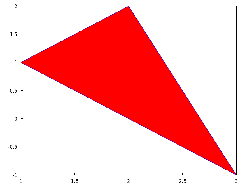
3D
triangle ([x1,y1,z1], [x2,y2,z2], [x3,y3,z3]) draws a triangle with vertices [x1,y1,z1],
[x2,y2,z2], and [x3,y3,z3].
This object is affected by the following graphic options: line_type,
line_width, color, key, enhanced3d and transform.
See also: transparent, fill_color, border, line_width, key, xaxis_secondary, yaxis_secondary, line_type, transform, color, enhanced3d.
tube (xfun, yfun, zfun, rfun, p, pmin, pmax) — Function
Draws a tube in 3D with varying diameter.
3D
[xfun,yfun,zfun]
is the parametric curve with parameter p taking values from pmin
to pmax. Circles of radius rfun are placed with their centers on
the parametric curve and perpendicular to it.
This object is affected by the following graphic options: xu_grid,
yv_grid, line_type, line_width, key, wired_surface, enhanced3d,
color and capping.
Example:
(%i1) draw3d(
        enhanced3d = true,
        xu_grid = 50,
        tube(cos(a), a, 0, cos(a/10)^2,
             a, 0, 4*%pi) )$
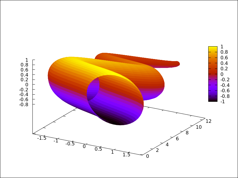
See also: xu_grid, yv_grid, line_type, line_width, key, wired_surface, enhanced3d, color, capping.
unit_vectors — Variable
Default value: false
If unit_vectors is true, vectors are plotted with module 1.
This is useful for plotting vector fields. If unit_vectors is false,
vectors are plotted with its original length.
This option is relevant only for vector objects.
Example:
(%i1) draw2d(xrange      = [-1,6],
             yrange      = [-1,6],
             head_length = 0.1,
             vector([0,0],[5,2]),
             unit_vectors = true,
             color        = red,
             vector([0,3],[5,2]))$
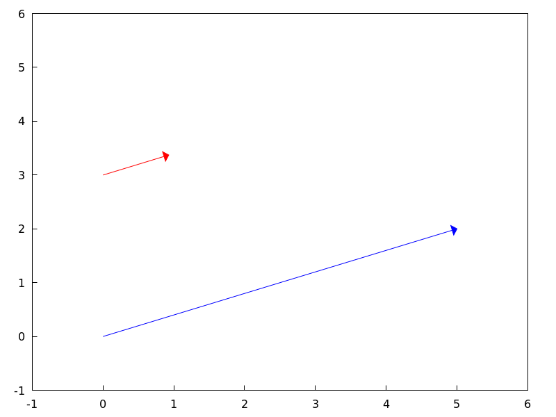
user_preamble — Variable
Default value: "" (empty string)
Expert Gnuplot users can make use of this option to fine tune Gnuplot’s
behaviour by writing settings to be sent before the plot or splot
command.
The value of this option must be a string or a list of strings (one per line).
Since this is a global graphics option, its position in the scene description does not matter.
Example:
Tell Gnuplot to draw axes and grid on top of graphics objects,
(%i1) draw2d(
        xaxis =true, xaxis_type=solid,
        yaxis =true, yaxis_type=solid,
        user_preamble="set grid front",
        region(x^2+y^2<1 ,x,-1.5,1.5,y,-1.5,1.5))$
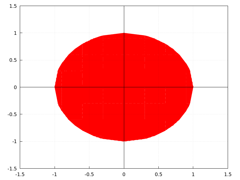
Tell gnuplot to draw all contour lines in black
(%i1) draw3d(
          contour=both,
          surface_hide=true,enhanced3d=true,wired_surface=true,
          contour_levels=10,
          user_preamble="set for [i=1:8] linetype i dashtype i linecolor 0",
          explicit(sin(x)*cos(y),x,1,10,y,1,10)
      );
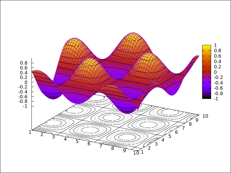
vector ([x, y], [dx, dy]) — Function
Draws vectors in 2D and 3D.
This object is affected by the following graphic options: head_both,
head_length, head_angle, head_type, line_width,
line_type, key and color.
2D
vector([x,y], [dx,dy]) plots vector
[dx,dy] with origin in [x,y].
Example:
(%i1) draw2d(xrange      = [0,12],
             yrange      = [0,10],
             head_length = 1,
             vector([0,1],[5,5]), /* default type */
             head_type = 'empty,
             vector([3,1],[5,5]),
             head_both = true,
             head_type = 'nofilled,
             line_type = dots,
             vector([6,1],[5,5]))$
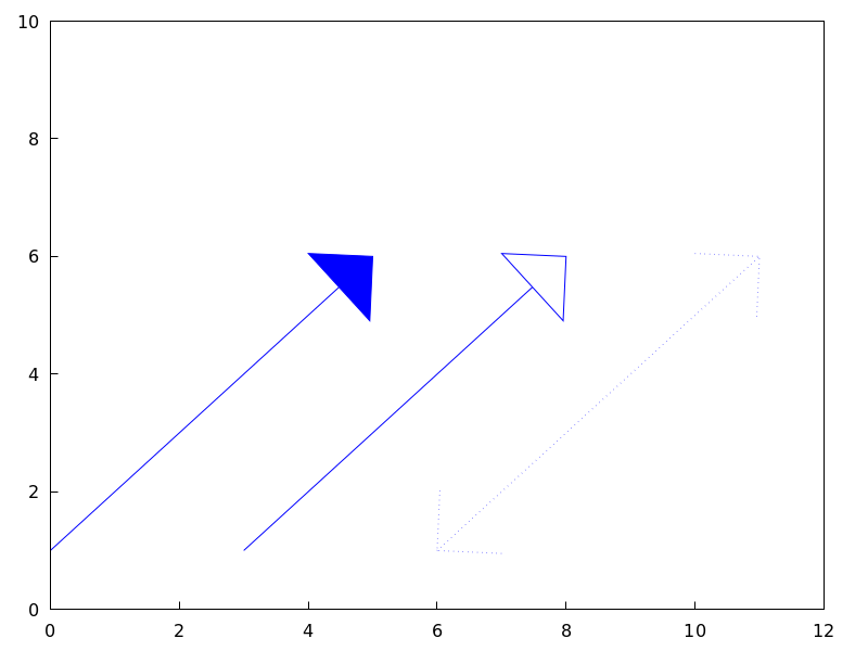
3D
vector([x,y,z], [dx,dy,dz])
plots vector [dx,dy,dz] with
origin in [x,y,z].
Example:
(%i1) draw3d(color = cyan,
             vector([0,0,0],[1,1,1]/sqrt(3)),
             vector([0,0,0],[1,-1,0]/sqrt(2)),
             vector([0,0,0],[1,1,-2]/sqrt(6)) )$
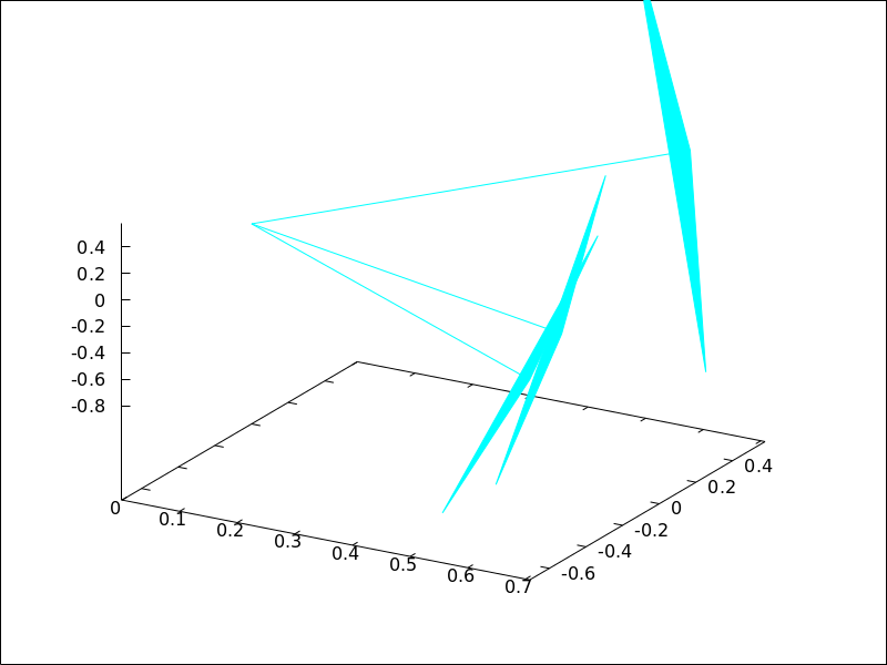
See also: head_both, head_length, head_angle, head_type, line_width, line_type, key.
view — Variable
Default value: [60,30]
A pair of angles, measured in degrees, indicating the view direction in a 3D scene. The first angle is the vertical rotation around the x axis, in the range $[0, 360]$. The second one is the horizontal rotation around the z axis, in the range $[0, 360]$.
If option view is given the value map, the view direction is set
to be perpendicular to the xy-plane.
Since this is a global graphics option, its position in the scene description does not matter.
Example:
(%i1) draw3d(view = [170, 50],
             enhanced3d = true,
             explicit(sin(x^2+y^2),x,-2,2,y,-2,2) )$
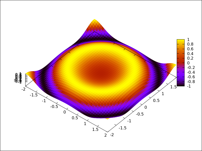
(%i2) draw3d(view = map,
             enhanced3d = true,
             explicit(sin(x^2+y^2),x,-2,2,y,-2,2) )$
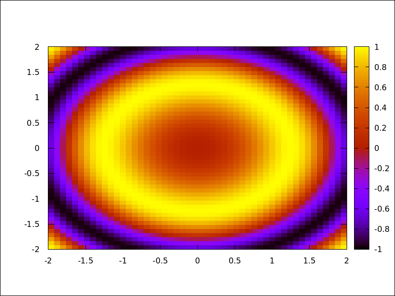
wired_surface — Variable
Default value: false
Indicates whether 3D surfaces in enhanced3d mode show the grid joining
the points or not.
Since this is a global graphics option, its position in the scene description does not matter.
Example:
(%i1) draw3d(
        enhanced3d    = [sin(x),x,y],
        wired_surface = true,
        explicit(x^2+y^2,x,-1,1,y,-1,1)) $
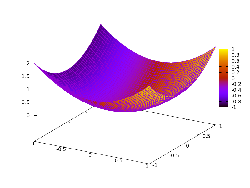
x_voxel — Variable
Default value: 10
x_voxel is the number of voxels in the x direction to
be used by the marching cubes algorithm implemented
by the 3d implicit object. It is also used by graphic
object region.
See also: region.
xaxis — Variable
Default value: false
If xaxis is true, the x axis is drawn.
Since this is a global graphics option, its position in the scene description does not matter.
Example:
(%i1) draw2d(explicit(x^3,x,-1,1),
             xaxis       = true,
             xaxis_color = blue)$
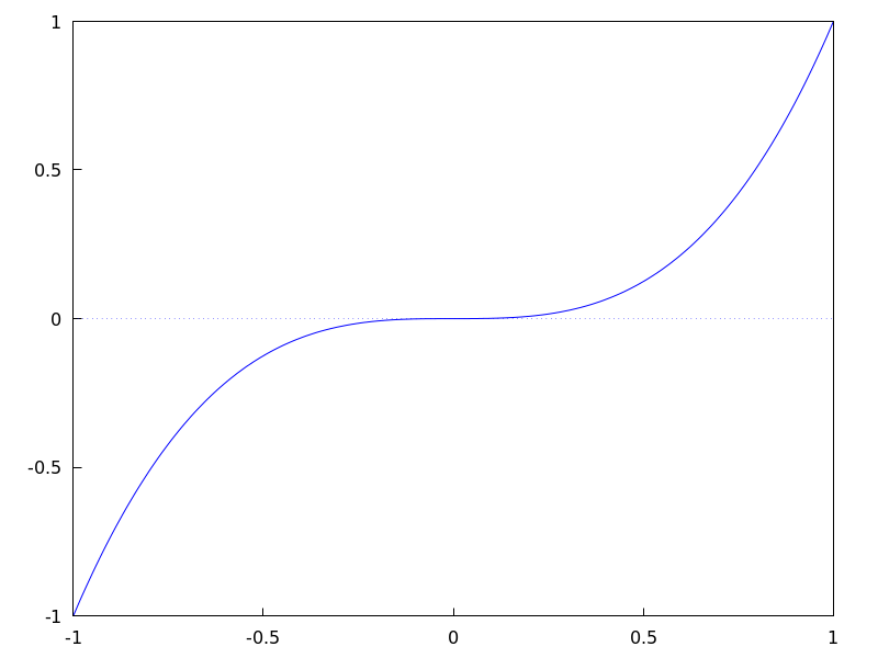
See also xaxis_width, xaxis_type and xaxis_005fcolor.
See also: xaxis_width, xaxis_type, xaxis_color.
xaxis_color — Variable
Default value: "black"
xaxis_color specifies the color for the x axis. See
color to know how colors are defined.
Since this is a global graphics option, its position in the scene description does not matter.
Example:
(%i1) draw2d(explicit(x^3,x,-1,1),
             xaxis       = true,
             xaxis_color = red)$
See also xaxis, xaxis_width and xaxis_005ftype.
See also: xaxis, xaxis_width, xaxis_type.
xaxis_secondary — Variable
Default value: false
If xaxis_secondary is true, function values can be plotted with
respect to the second x axis, which will be drawn on top of the scene.
Note that this is a local graphics option which only affects to 2d plots.
Example:
(%i1) draw2d(
         key   = "Bottom x-axis",
         explicit(x+1,x,1,2),
         color = red,
         key   = "Above x-axis",
         xtics_secondary = true,
         xaxis_secondary = true,
         explicit(x^2,x,-1,1)) $
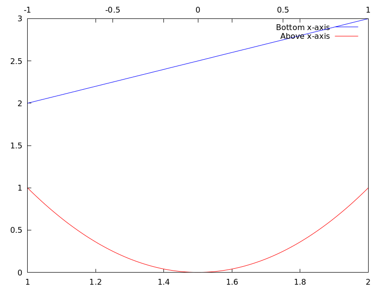
See also xrange_secondary, xtics_secondary, xtics_rotate_secondary,
xtics_axis_secondary and xaxis_005fsecondary.
See also: xrange_secondary, xtics_secondary, xtics_rotate_secondary, xaxis_secondary.
xaxis_type — Variable
Default value: dots
xaxis_type indicates how the x axis is displayed;
possible values are solid and dots
Since this is a global graphics option, its position in the scene description does not matter.
Example:
(%i1) draw2d(explicit(x^3,x,-1,1),
             xaxis       = true,
             xaxis_type  = solid)$
See also xaxis, xaxis_width and xaxis_005fcolor.
See also: xaxis, xaxis_width, xaxis_color.
xaxis_width — Variable
Default value: 1
xaxis_width is the width of the x axis.
Its value must be a positive number.
Since this is a global graphics option, its position in the scene description does not matter.
Example:
(%i1) draw2d(explicit(x^3,x,-1,1),
             xaxis       = true,
             xaxis_width = 3)$
See also xaxis, xaxis_type and xaxis_005fcolor.
See also: xaxis, xaxis_type, xaxis_color.
xlabel_secondary — Variable
Default value: "" (empty string)
Option xlabel_secondary, a string, is the label for the secondary x axis.
By default, no label is written.
Since this is a global graphics option, its position in the scene description does not matter.
Example:
(%i1) draw2d(
         xaxis_secondary=true,yaxis_secondary=true,
         xtics_secondary=true,ytics_secondary=true,
         xlabel_secondary="t[s]",
         ylabel_secondary="U[V]",
         explicit(sin(t),t,0,10) )$
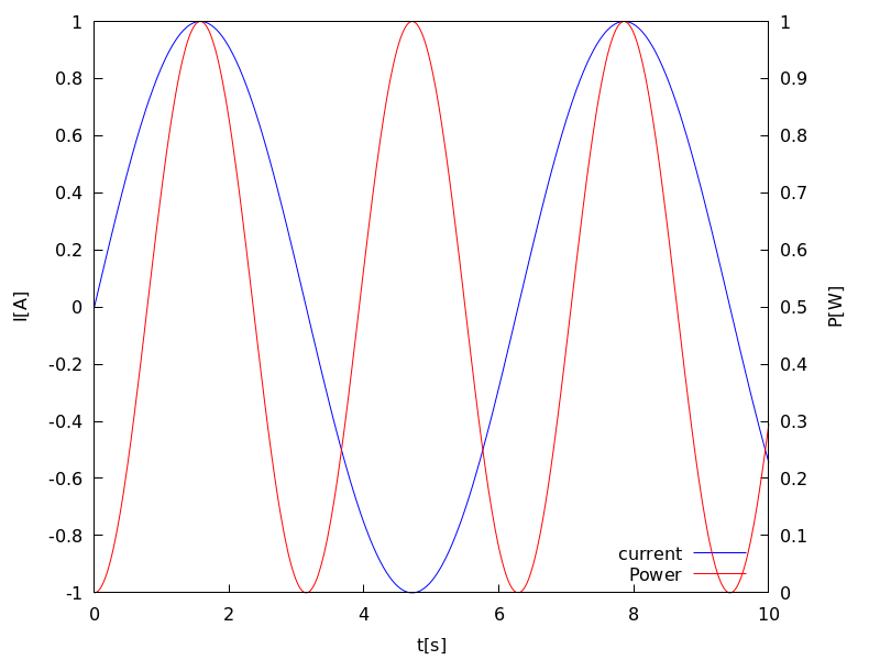
See also xlabel_draw, ylabel_draw, ylabel_secondary and zlabel_005fdraw.
See also: xlabel_draw, ylabel_draw, ylabel_secondary, zlabel_draw.
xrange — Variable
Default value: auto
If xrange is auto, the range for the x coordinate is
computed automatically.
If the user wants a specific interval for x, it must be given as a
Maxima list, as in xrange=[-2, 3].
Since this is a global graphics option, its position in the scene description does not matter.
Example:
(%i1) draw2d(xrange = [-3,5],
             explicit(x^2,x,-1,1))$
See also yrange and zrange.
See also: yrange, zrange.
xrange_secondary — Variable
Default value: auto
If xrange_secondary is auto, the range for the second x axis is
computed automatically.
If the user wants a specific interval for the second x axis, it must be given as a
Maxima list, as in xrange_secondary=[-2, 3].
Since this is a global graphics option, its position in the scene description does not matter.
See also xrange, yrange, zrange and yrange_005fsecondary.
See also: xrange, yrange, zrange, yrange_secondary.
xtics_axis — Variable
Default value: false
If xtics_axis is true, tic marks and their labels are plotted just
along the x axis, if it is false tics are plotted on the border.
Since this is a global graphics option, its position in the scene description does not matter.
xtics_rotate — Variable
Default value: false
If xtics_rotate is true, tic marks on the x axis are rotated
90 degrees.
Since this is a global graphics option, its position in the scene description does not matter.
xtics_rotate_secondary — Variable
Default value: false
If xtics_rotate_secondary is true, tic marks on the secondary x axis are rotated
90 degrees.
Since this is a global graphics option, its position in the scene description does not matter.
xtics_secondary — Variable
Default value: auto
This graphic option controls the way tic marks are drawn on the second x axis.
See xtics_draw for a complete description.
See also: xtics_draw.
xtics_secondary_axis — Variable
Default value: false
If xtics_secondary_axis is true, tic marks and their labels are plotted just
along the secondary x axis, if it is false tics are plotted on the border.
Since this is a global graphics option, its position in the scene description does not matter.
xu_grid — Variable
Default value: 30
xu_grid is the number of coordinates of the first variable
(x in explicit and u in parametric 3d surfaces) to
build the grid of sample points.
This option affects the following graphic objects:
gr3d: explicit and parametric_surface.
Example:
(%i1) draw3d(xu_grid = 10,
             yv_grid = 50,
             explicit(x^2+y^2,x,-3,3,y,-3,3) )$
See also yv_005fgrid.
See also: yv_grid.
xy_file — Variable
Default value: "" (empty string)
xy_file is the name of the file where the coordinates will be saved
after clicking with the mouse button and hitting the ’x’ key. By default,
no coordinates are saved.
Since this is a global graphics option, its position in the scene description does not matter.
xyplane — Variable
Default value: false
Allocates the xy-plane in 3D scenes. When xyplane is
false, the xy-plane is placed automatically; when it is
a real number, the xy-plane intersects the z-axis at this level.
This option has no effect in 2D scenes.
Since this is a global graphics option, its position in the scene description does not matter.
Example:
(%i1) draw3d(xyplane = %e-2,
             explicit(x^2+y^2,x,-1,1,y,-1,1))$
y_voxel — Variable
Default value: 10
y_voxel is the number of voxels in the y direction to
be used by the marching cubes algorithm implemented
by the 3d implicit object. It is also used by graphic
object region.
See also: region.
yaxis — Variable
Default value: false
If yaxis is true, the y axis is drawn.
Since this is a global graphics option, its position in the scene description does not matter.
Example:
(%i1) draw2d(explicit(x^3,x,-1,1),
             yaxis       = true,
             yaxis_color = blue)$
See also yaxis_width, yaxis_type and yaxis_005fcolor.
See also: yaxis_width, yaxis_type, yaxis_color.
yaxis_color — Variable
Default value: "black"
yaxis_color specifies the color for the y axis. See
color to know how colors are defined.
Since this is a global graphics option, its position in the scene description does not matter.
Example:
(%i1) draw2d(explicit(x^3,x,-1,1),
             yaxis       = true,
             yaxis_color = red)$
See also yaxis, yaxis_width and yaxis_005ftype.
See also: yaxis, yaxis_width, yaxis_type.
yaxis_secondary — Variable
Default value: false
If yaxis_secondary is true, function values can be plotted with
respect to the second y axis, which will be drawn on the right side of the
scene.
Note that this is a local graphics option which only affects to 2d plots.
Example:
(%i1) draw2d(
         explicit(sin(x),x,0,10),
         yaxis_secondary = true,
         ytics_secondary = true,
         color = blue,
         explicit(100*sin(x+0.1)+2,x,0,10));
See also yrange_secondary, ytics_secondary, ytics_rotate_secondary
and ytics_axis_secondary
See also: yrange_secondary, ytics_secondary, ytics_rotate_secondary.
yaxis_type — Variable
Default value: dots
yaxis_type indicates how the y axis is displayed;
possible values are solid and dots.
Since this is a global graphics option, its position in the scene description does not matter.
Example:
(%i1) draw2d(explicit(x^3,x,-1,1),
             yaxis       = true,
             yaxis_type  = solid)$
See also yaxis, yaxis_width and yaxis_005fcolor.
See also: yaxis, yaxis_width, yaxis_color.
yaxis_width — Variable
Default value: 1
yaxis_width is the width of the y axis.
Its value must be a positive number.
Since this is a global graphics option, its position in the scene description does not matter.
Example:
(%i1) draw2d(explicit(x^3,x,-1,1),
             yaxis       = true,
             yaxis_width = 3)$
See also yaxis, yaxis_type and yaxis_005fcolor.
See also: yaxis, yaxis_type, yaxis_color.
ylabel_secondary — Variable
Default value: "" (empty string)
Option ylabel_secondary, a string, is the label for the secondary y axis.
By default, no label is written.
Since this is a global graphics option, its position in the scene description does not matter.
Example:
(%i1) draw2d(
        key_pos=bottom_right,
        key="current",
        xlabel="t[s]",
        ylabel="I[A]",ylabel_secondary="P[W]",
        explicit(sin(t),t,0,10),
        yaxis_secondary=true,
        ytics_secondary=true,
        color=red,key="Power",
        explicit((sin(t))^2,t,0,10)
    )$
See also xlabel_draw, xlabel_secondary, ylabel_draw and zlabel_005fdraw.
See also: xlabel_draw, xlabel_secondary, ylabel_draw, zlabel_draw.
yrange — Variable
Default value: auto
If yrange is auto, the range for the y coordinate is
computed automatically.
If the user wants a specific interval for y, it must be given as a
Maxima list, as in yrange=[-2, 3].
Since this is a global graphics option, its position in the scene description does not matter.
Example:
(%i1) draw2d(yrange = [-2,3],
             explicit(x^2,x,-1,1),
             xrange = [-3,3])$
See also xrange, yrange_secondary and zrange.
See also: xrange, yrange_secondary, zrange.
yrange_secondary — Variable
Default value: auto
If yrange_secondary is auto, the range for the second y axis is
computed automatically.
If the user wants a specific interval for the second y axis, it must be given as a
Maxima list, as in yrange_secondary=[-2, 3].
Since this is a global graphics option, its position in the scene description does not matter.
Example:
(%i1) draw2d(
         explicit(sin(x),x,0,10),
         yaxis_secondary = true,
         ytics_secondary = true,
         yrange = [-3, 3],
         yrange_secondary = [-20, 20],
         color = blue,
         explicit(100*sin(x+0.1)+2,x,0,10)) $
See also xrange, yrange and zrange.
See also: xrange, yrange, zrange.
ytics_axis — Variable
Default value: false
If ytics_axis is true, tic marks and their labels are plotted just
along the y axis, if it is false tics are plotted on the border.
Since this is a global graphics option, its position in the scene description does not matter.
ytics_rotate — Variable
Default value: false
If ytics_rotate is true, tic marks on the y axis are rotated
90 degrees.
Since this is a global graphics option, its position in the scene description does not matter.
ytics_rotate_secondary — Variable
Default value: false
If ytics_rotate_secondary is true, tic marks on the secondary y axis are rotated
90 degrees.
Since this is a global graphics option, its position in the scene description does not matter.
ytics_secondary — Variable
Default value: auto
This graphic option controls the way tic marks are drawn on the second y axis.
See xtics for a complete description.
ytics_secondary_axis — Variable
Default value: false
If ytics_secondary_axis is true, tic marks and their labels are plotted just
along the secondary y axis, if it is false tics are plotted on the border.
Since this is a global graphics option, its position in the scene description does not matter.
yv_grid — Variable
Default value: 30
yv_grid is the number of coordinates of the second variable
(y in explicit and v in parametric 3d surfaces) to
build the grid of sample points.
This option affects the following graphic objects:
gr3d: explicit and parametric_surface.
Example:
(%i1) draw3d(xu_grid = 10,
             yv_grid = 50,
             explicit(x^2+y^2,x,-3,3,y,-3,3) )$
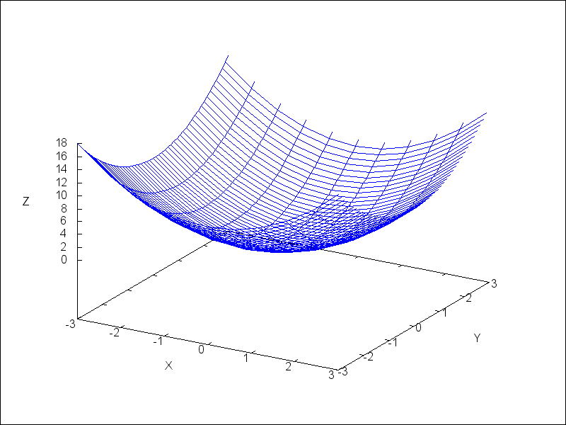
See also xu_005fgrid.
See also: explicit, parametric_surface, xu_grid.
z_voxel — Variable
Default value: 10
z_voxel is the number of voxels in the z direction to
be used by the marching cubes algorithm implemented
by the 3d implicit object.
zaxis — Variable
Default value: false
If zaxis is true, the z axis is drawn in 3D plots.
This option has no effect in 2D scenes.
Since this is a global graphics option, its position in the scene description does not matter.
Example:
(%i1) draw3d(explicit(x^2+y^2,x,-1,1,y,-1,1),
             zaxis       = true,
             zaxis_type  = solid,
             zaxis_color = blue)$
See also zaxis_width, zaxis_type and zaxis_005fcolor.
See also: zaxis_width, zaxis_type, zaxis_color.
zaxis_color — Variable
Default value: "black"
zaxis_color specifies the color for the z axis. See
color to know how colors are defined.
This option has no effect in 2D scenes.
Since this is a global graphics option, its position in the scene description does not matter.
Example:
(%i1) draw3d(explicit(x^2+y^2,x,-1,1,y,-1,1),
             zaxis       = true,
             zaxis_type  = solid,
             zaxis_color = red)$
See also zaxis, zaxis_width and zaxis_005ftype.
See also: zaxis, zaxis_width, zaxis_type.
zaxis_type — Variable
Default value: dots
zaxis_type indicates how the z axis is displayed;
possible values are solid and dots.
This option has no effect in 2D scenes.
Since this is a global graphics option, its position in the scene description does not matter.
Example:
(%i1) draw3d(explicit(x^2+y^2,x,-1,1,y,-1,1),
             zaxis       = true,
             zaxis_type  = solid)$
See also zaxis, zaxis_width and zaxis_005fcolor.
See also: zaxis, zaxis_width, zaxis_color.
zaxis_width — Variable
Default value: 1
zaxis_width is the width of the z axis.
Its value must be a positive number. This option has no effect in 2D scenes.
Since this is a global graphics option, its position in the scene description does not matter.
Example:
(%i1) draw3d(explicit(x^2+y^2,x,-1,1,y,-1,1),
             zaxis       = true,
             zaxis_type  = solid,
             zaxis_width = 3)$
See also zaxis, zaxis_type and zaxis_005fcolor.
See also: zaxis, zaxis_type, zaxis_color.
zlabel_rotate — Variable
Default value: "auto"
This graphics option allows to choose if the z axis label of 3d plots is
drawn horizontal (false), vertical (true) or if maxima
automatically chooses an orientation based on the length of the label
(auto).
Since this is a global graphics option, its position in the scene description does not matter.
Example:
(%i1) draw3d(
          explicit(sin(x)*sin(y),x,0,10,y,0,10),
          zlabel_rotate=false
      )$
See also zlabel_005fdraw.
See also: zlabel_draw.
zrange — Variable
Default value: auto
If zrange is auto, the range for the z coordinate is
computed automatically.
If the user wants a specific interval for z, it must be given as a
Maxima list, as in zrange=[-2, 3].
Since this is a global graphics option, its position in the scene description does not matter.
Example:
(%i1) draw3d(yrange = [-3,3],
             zrange = [-2,5],
             explicit(x^2+y^2,x,-1,1,y,-1,1),
             xrange = [-3,3])$
See also xrange and yrange.
See also: xrange, yrange.
ztics_axis — Variable
Default value: false
If ztics_axis is true, tic marks and their labels are plotted just
along the z axis, if it is false tics are plotted on the border.
Since this is a global graphics option, its position in the scene description does not matter.
ztics_rotate — Variable
Default value: false
If ztics_rotate is true, tic marks on the z axis are rotated
90 degrees.
Since this is a global graphics option, its position in the scene description does not matter.